Simultaneous Tracking and Recognizing Drone Targets with Millimeter-Wave Radar and Convolutional Neural Network


Abstract
:1. Introduction
- A signal-processing algorithm is proposed to generate 3D point clouds of multiple moving targets in the field of view (FoV), considering both static and dynamic reflections of mmWave radar signals.
- A multitarget tracking algorithm was developed that integrates a density-based clustering algorithm to merge related point clouds into clusters, extended Kalman filters (EKF) to estimate the new position of the detected targets, and the Hungarian algorithm to match each new estimated track with its target cluster.
- A novel CNN model is proposed for feature extraction and identification of drone and non-drone targets from clustered 3D cloud points.
- The performance of the proposed tracking and recognition algorithms was evaluated.
2. Related Works
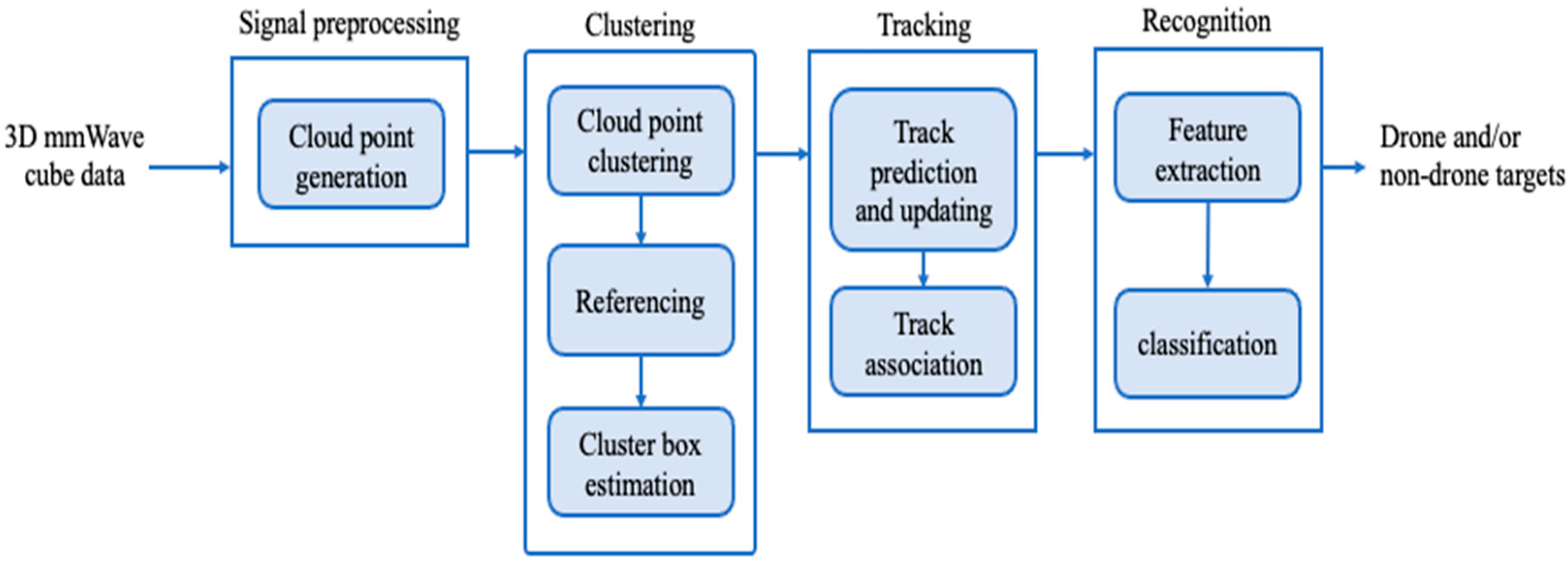
3. The Proposed Framework
- 5.
- Signal preprocessing: This module translates the raw information collected by the mmWave radar into sparse point clouds and eliminates the points associated with interference noises and static objects (i.e., points that appeared in the previous frame), which reveal the existence and movement of targets.
- 6.
- Clustering: This module detects different moving targets and merges the related point clouds into clusters, where each cluster represents a single moving target.
- 7.
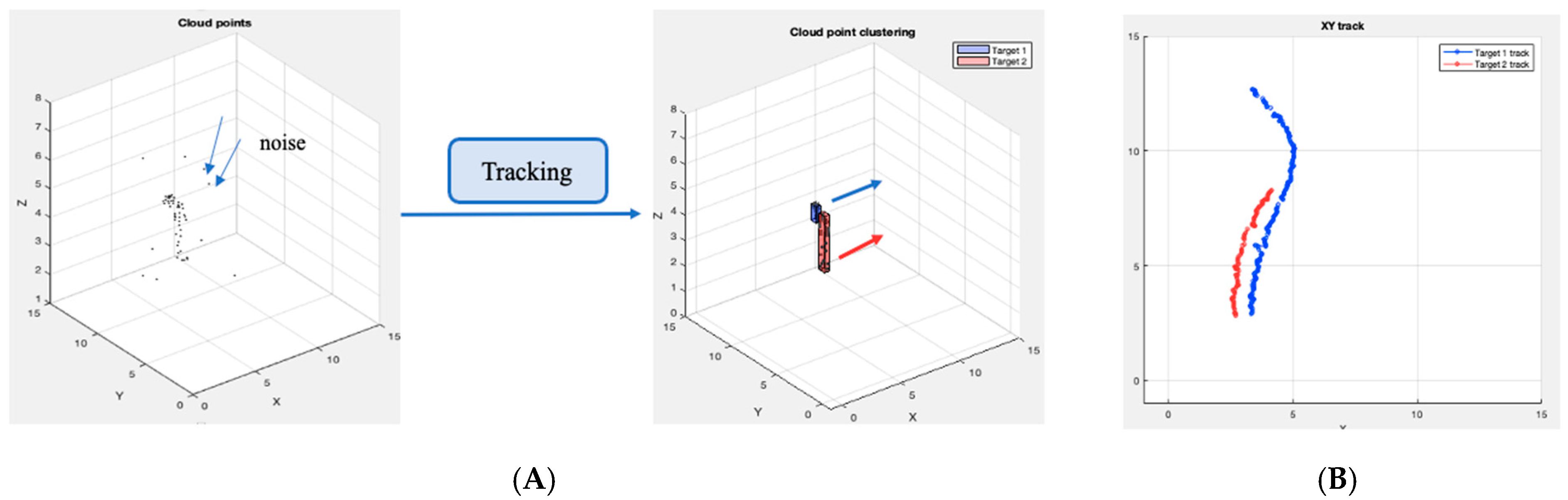
- Tracking: This module estimates a target track in successive frames and applies an association algorithm to track multiple targets’ paths.
- 8.
- Recognition: This module utilizes a CNN model to extract representative spatiotemporal features from cloud points and then classifies the detected targets as drone and non-drone targets.
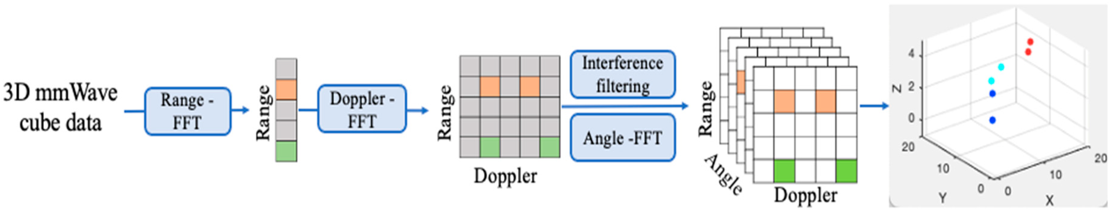
4. Signal Preprocessing
4.1. Range Fast Fourier Transform
4.2. Doppler Fast Fourier Transform
4.3. Interference Filtering
4.3.1. CFAR Algorithm
4.3.2. MTI Algorithm
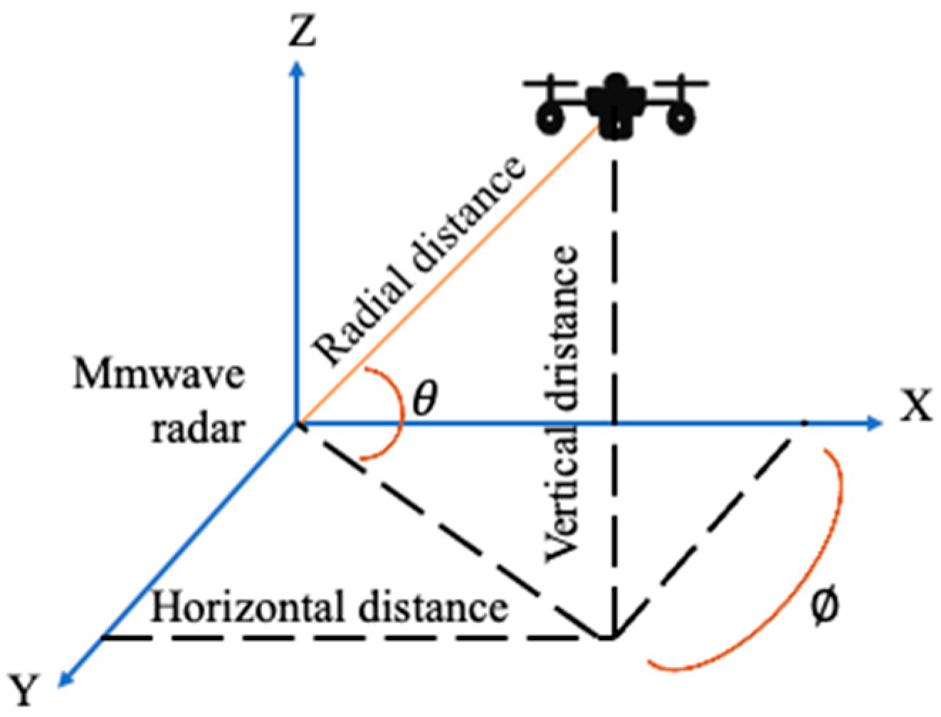
4.4. Angle Fourier Transform
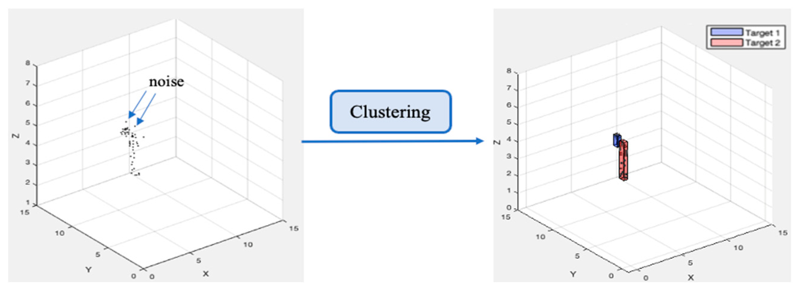
5. Clustering
5.1. Cloud Point Clustering
| Algorithm 1 Clustering algorithm. |
| Input: : the largest Euclidean distance between two points; the minimum number of points required for a cluster. Output: clustered targets 1. Initialize the values of and . 2. Choose point randomly, which is not identified as a cluster or noise. 3. Calculate its neighboring points to determine whether it is a primary point. If this is true, form a cluster surrounding this point; otherwise, this point is considered noise. 4. If is a primary point, a cluster is formed, enlarging the cluster by including points that are reachable by it and are less than 5. If a noise point is added, change the status of that point from noise to a boundary point. 6. Continue with Steps 2:5 until all points have been designated as cluster points or noise. |
5.2. Referencing
| Algorithm 2 Centroid-determining algorithm. |
| Input: cloud point clusters. Output: centroid of each cluster For each cluster: 1. Choose a point as a centroid randomly. 2. Assign all remaining points as non-centroids represented by the nearest centroid. 3. Choose a non-centroid point randomly selected in every cluster. 4. Let each current centroid denoted as . 5. To form the new centroid, calculate the cost of exchanging with , involving the cost of reassigning non-centroid points caused by the exchange if , and then, exchange , with . 6. Repeat Step 3:5 until no change. |
5.3. Cluster Box Estimation
6. Tracking
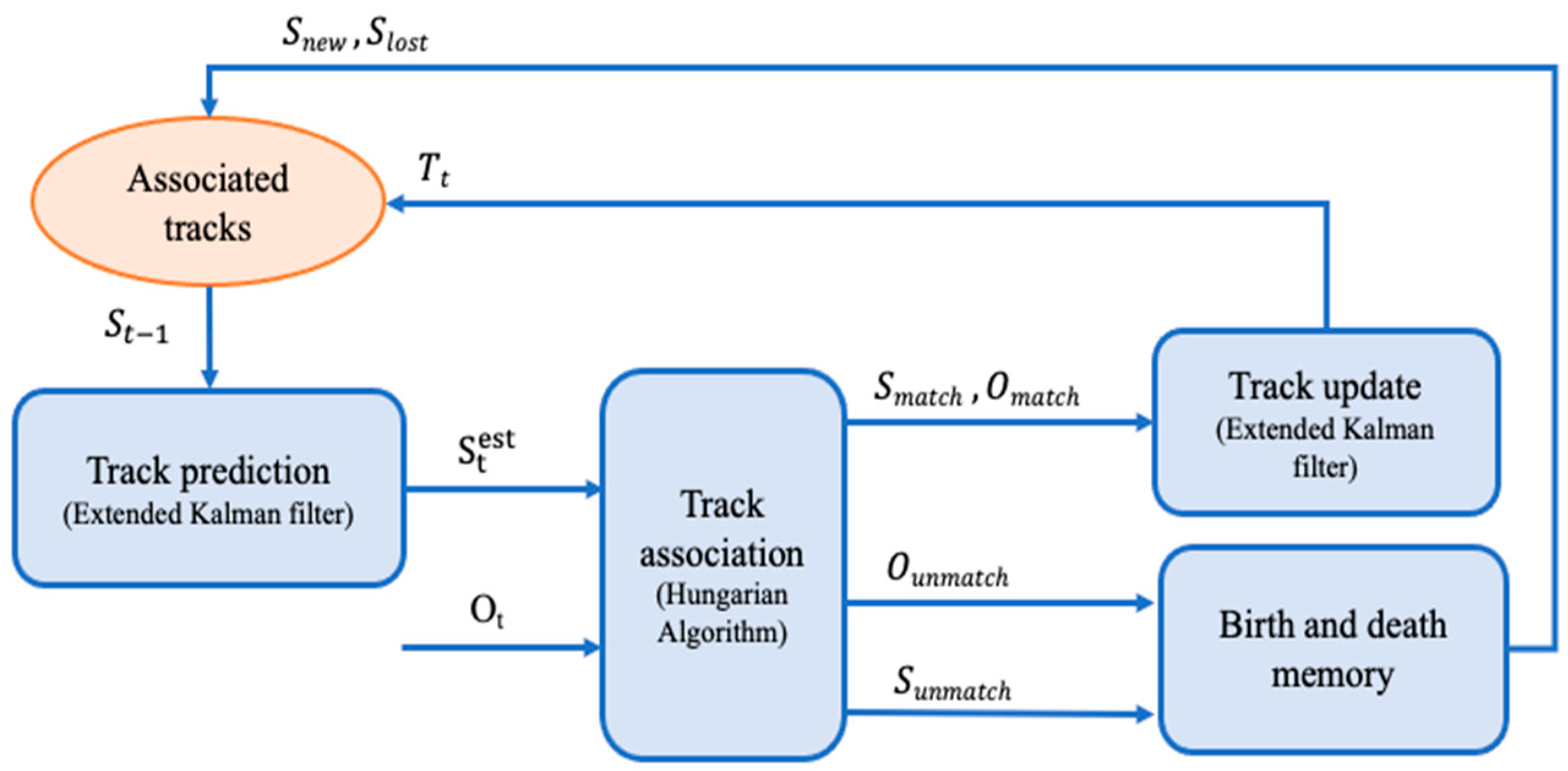
6.1. Track Estimation and Updating
6.2. Track Association
6.3. Birth and Death
7. Recognition
CNN Model for Feature Extraction and Classification
8. Performance Evaluation
8.1. Clustering
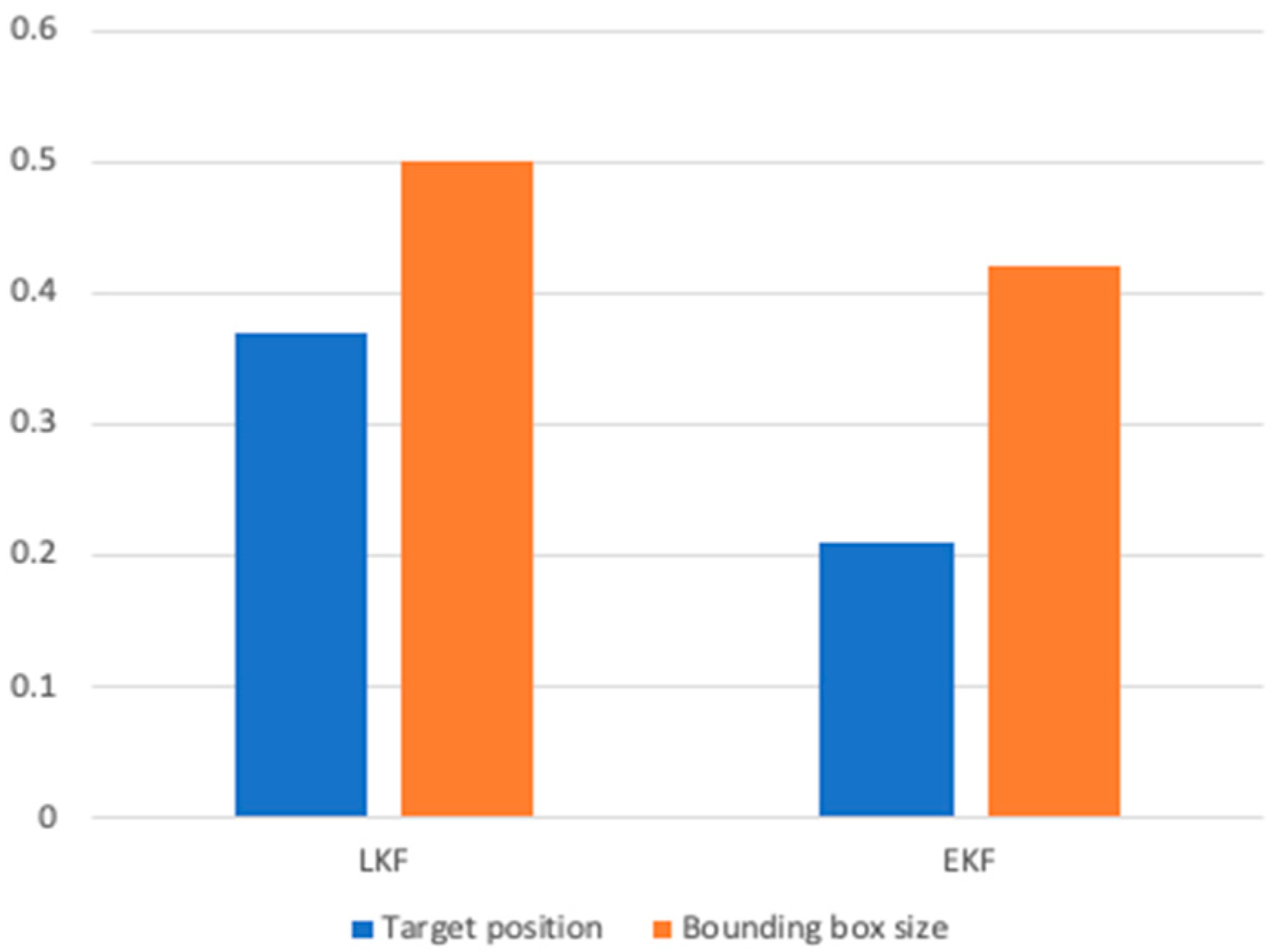
8.2. Tracking
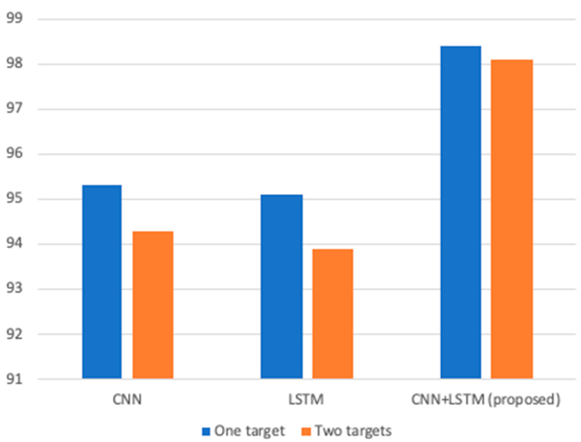
8.3. Recognition
9. Conclusions and Future Work
Author Contributions
Funding
Data Availability Statement
Conflicts of Interest
References
- Kanellakis, C.; Nikolakopoulos, G. Survey on computer vision for UAVs: Current developments and trends. J. Intell. Robot. Syst. 2017, 87, 141–168. [Google Scholar]
- Fu, R.; Al-Absi, M.A.; Kim, K.-H.; Lee, Y.-S.; Al-Absi, A.A.; Lee, H.-J. Deep Learning-Based Drone Classification Using Radar Cross Section Signatures at mmWave Frequencies. IEEE Access 2021, 9, 161431–161444. [Google Scholar]
- Doole, M.; Ellerbroek, J.; Hoekstra, J. Estimation of traffic density from drone-based delivery in very low level urban airspace. J. Air Transp. Manag. 2020, 88, 101862. [Google Scholar]
- Brahim, I.B.; Addouche, S.-A.; El Mhamedi, A.; Boujelbene, Y. Cluster-based WSA method to elicit expert knowledge for Bayesian reasoning—Case of parcel delivery with drone. Expert Syst. Appl. 2022, 191, 116160. [Google Scholar]
- Sinhababu, N.; Pramanik, P.K.D. An Efficient Obstacle Detection Scheme for Low-Altitude UAVs Using Google Maps. In Data Management, Analytics and Innovation; Springer: Berlin/Heidelberg, Germany, 2022; pp. 455–470. [Google Scholar]
- Cheng, M.-L.; Matsuoka, M.; Liu, W.; Yamazaki, F. Near-real-time gradually expanding 3D land surface reconstruction in disaster areas by sequential drone imagery. Autom. Constr. 2022, 135, 104105. [Google Scholar]
- Rizk, H.; Nishimur, Y.; Yamaguchi, H.; Higashino, T. Drone-Based Water Level Detection in Flood Disasters. Int. J. Environ. Res. Public Health 2022, 19, 237. [Google Scholar]
- Nath, N.D.; Cheng, C.-S.; Behzadan, A.H. Drone mapping of damage information in GPS-Denied disaster sites. Adv. Eng. Inform. 2022, 51, 101450. [Google Scholar]
- Mishra, B.; Garg, D.; Narang, P.; Mishra, V. Drone-surveillance for search and rescue in natural disaster. Comput. Commun. 2020, 156, 1–10. [Google Scholar] [CrossRef]
- Jacob, B.; Kaushik, A.; Velavan, P. Autonomous Navigation of Drones Using Reinforcement Learning. In Advances in Augmented Reality and Virtual Reality; Springer: Berlin/Heidelberg, Germany, 2022; pp. 159–176. [Google Scholar]
- Chechushkov, I.V.; Ankusheva, P.S.; Ankushev, M.N.; Bazhenov, E.A.; Alaeva, I.P. Assessment of Excavated Volume and Labor Investment at the Novotemirsky Copper Ore Mining Site. In Geoarchaeology and Archaeological Mineralogy; Springer: Berlin/Heidelberg, Germany, 2022; pp. 199–205. [Google Scholar]
- Molnar, P. Territorial and Digital Borders and Migrant Vulnerability Under a Pandemic Crisis. In Migration and Pandemics; Springer: Cham, Switzerland, 2022; pp. 45–64. [Google Scholar]
- Sharma, N.; Saqib, M.; Scully-Power, P.; Blumenstein, M. SharkSpotter: Shark Detection with Drones for Human Safety and Environmental Protection. In Humanity Driven AI; Springer: Berlin/Heidelberg, Germany, 2022; pp. 223–237. [Google Scholar]
- Bhatia, J.; Dayal, A.; Jha, A.; Vishvakarma, S.K.; Soumya, J.; Srinivas, M.B.; Yalavarthy, P.K.; Kumar, A.; Lalitha, V.; Koorapati, S. Object Classification Technique for mmWave FMCW Radars using Range-FFT Features. In Proceedings of the 2021 International Conference on COMmunication Systems & NETworkS (COMSNETS), Bangalore, India, 5–9 January 2021; pp. 111–115. [Google Scholar]
- Huang, X.; Cheena, H.; Thomas, A.; Tsoi, J.K.P. Indoor Detection and Tracking of People Using mmWave Sensor. J. Sens. 2021, 2021, 6657709. [Google Scholar]
- Beringer, R.; Sixsmith, A.; Campo, M.; Brown, J.; McCloskey, R. The “acceptance” of ambient assisted living: Developing an alternate methodology to this limited research lens. In Towards Useful Services for Elderly and People with Disabilities, Proceedings of the International Conference on Smart Homes and Health Telematics, Montreal, QC, Canada, 20–22 June 2011; Springer: Berlin/Heidelberg, Germany, 2011; pp. 161–167. [Google Scholar]
- Ferris, D.D., Jr.; Currie, N.C. Microwave and millimeter-wave systems for wall penetration. In Targets and Backgrounds: Characterization and Representation IV; International Society for Optics and Photonics: Bellingham, WA, USA, 1998; Volume 3375, pp. 269–279. [Google Scholar]
- Zhao, P.; Lu, C.X.; Wang, J.; Chen, C.; Wang, W.; Trigoni, N.; Markham, A. mID: Tracking and identifying people with millimeter wave radar. In Proceedings of the 2019 15th International Conference on Distributed Computing in Sensor Systems (DCOSS), Santorini, Greece, 29–31 May 2019; pp. 33–40. [Google Scholar]
- Sengupta, A.; Jin, F.; Zhang, R.; Cao, S. mm-Pose: Real-time human skeletal posture estimation using mmWave radars and CNNs. IEEE Sens. J. 2020, 20, 10032–10044. [Google Scholar]
- Yang, Y.; Hou, C.; Lang, Y.; Yue, G.; He, Y.; Xiang, W. Person identification using micro-Doppler signatures of human motions and UWB radar. IEEE Microw. Wirel. Compon. Lett. 2019, 29, 366–368. [Google Scholar]
- Tripathi, S.; Kang, B.; Dane, G.; Nguyen, T. Low-complexity object detection with deep convolutional neural network for embedded systems. In Applications of Digital Image Processing XL; International Society for Optics and Photonics: Bellingham, WA, USA, 2017; Volume 10396, p. 103961M. [Google Scholar]
- Wang, S.; Song, J.; Lien, J.; Poupyrev, I.; Hilliges, O. Interacting with soli: Exploring fine-grained dynamic gesture recognition in the radio-frequency spectrum. In Proceedings of the 29th Annual Symposium on User Interface Software and Technology, Tokyo, Japan, 16–19 October 2016; pp. 851–860. [Google Scholar]
- Palipana, S.; Salami, D.; Leiva, L.A.; Sigg, S. Pantomime: Mid-air gesture recognition with sparse millimeter-wave radar point clouds. In Proceedings of the ACM on Interactive, Mobile, Wearable and Ubiquitous Technologies, New York, NY, USA, 21–26 September 2021; Volume 5, pp. 1–27. [Google Scholar]
- Srigrarom, S.; Sie, N.J.L.; Cheng, H.; Chew, K.H.; Lee, M.; Ratsamee, P. Multi-camera Multi-drone Detection, Tracking and Localization with Trajectory-based Re-identification. In Proceedings of the 2021 Second International Symposium on Instrumentation, Control, Artificial Intelligence, and Robotics (ICA-SYMP), Bangkok, Thailand, 20–22 January 2021; pp. 1–6. [Google Scholar]
- Al-Emadi, S.; Al-Ali, A.; Al-Ali, A. Audio-Based Drone Detection and Identification Using Deep Learning Techniques with Dataset Enhancement through Generative Adversarial Networks. Sensors 2021, 21, 4953. [Google Scholar] [PubMed]
- Alsoliman, A.; Rigoni, G.; Levorato, M.; Pinotti, C.; Tippenhauer, N.O.; Conti, M. COTS Drone Detection using Video Streaming Characteristics. In Proceedings of the 2021 International Conference on Distributed Computing and Networking, Nara, Japan, 5–8 January 2021; pp. 166–175. [Google Scholar]
- Rzewuski, S.; Kulpa, K.; Pachwicewicz, M.; Malanowski, M.; Salski, B. Drone Detectability Feasibility Study using Passive Radars Operating in WIFI and DVB-T Band; The Institute of Electronic Systems: Warsaw, PL, USA, 2021. [Google Scholar]
- Svanström, F.; Englund, C.; Alonso-Fernandez, F. Real-Time Drone Detection and Tracking with Visible, Thermal and Acoustic Sensors. In Proceedings of the 2020 25th International Conference on Pattern Recognition (ICPR), Milan, Italy, 10–15 January 2021; pp. 7265–7272. [Google Scholar]
- Yoo, L.-S.; Lee, J.-H.; Lee, Y.-K.; Jung, S.-K.; Choi, Y. Application of a Drone Magnetometer System to Military Mine Detection in the Demilitarized Zone. Sensors 2021, 21, 3175. [Google Scholar]
- Dogru, S.; Baptista, R.; Marques, L. Tracking drones with drones using millimeter wave radar. In Advances in Intelligent Systems and Computing, Proceedings of the Robot 2019: Fourth Iberian Robotics Conference, Porto, Portugal, 20–22 November 2019; Springer: Berlin/Heidelberg, Germany, 2019; pp. 392–402. [Google Scholar]
- Semkin, V.; Yin, M.; Hu, Y.; Mezzavilla, M.; Rangan, S. Drone detection and classification based on radar cross section signatures. In Proceedings of the 2020 International Symposium on Antennas and Propagation (ISAP), Osaka, Japan, 25–28 January 2021; pp. 223–224. [Google Scholar]
- Rai, P.K.; Idsøe, H.; Yakkati, R.R.; Kumar, A.; Khan, M.Z.A.; Yalavarthy, P.K.; Cenkeramaddi, L.R. Localization and Activity Classification of Unmanned Aerial Vehicle using mmWave FMCW Radars. IEEE Sens. J. 2021, 21, 16043–16053. [Google Scholar]
- Rahman, S.; Robertson, D.A. FAROS-E: A compact and low-cost millimeter wave surveillance radar for real time drone detection and classification. In Proceedings of the 2021 21st International Radar Symposium (IRS), Berlin, Germany, 21–22 June 2021; pp. 1–6. [Google Scholar]
- Jokanovic, B.; Amin, M.G.; Ahmad, F. Effect of data representations on deep learning in fall detection. In Proceedings of the 2016 IEEE Sensor Array and Multichannel Signal Processing Workshop (SAM), Rio de Janeiro, Brazil, 10–13 July 2016; pp. 1–5. [Google Scholar]
- Li, J.; Yang, B.; Chen, C.; Habib, A. NRLI-UAV: Non-rigid registration of sequential raw laser scans and images for low-cost UAV LiDAR point cloud quality improvement. ISPRS J. Photogramm. Remote Sens. 2019, 158, 123–145. [Google Scholar]
- Molchanov, P.; Gupta, S.; Kim, K.; Pulli, K. Short-range FMCW monopulse radar for hand-gesture sensing. In Proceedings of the 2015 IEEE Radar Conference (RadarCon), Arlington, VA, USA, 10–15 May 2015; pp. 1491–1496. [Google Scholar]
- Janakaraj, P.; Jakkala, K.; Bhuyan, A.; Sun, Z.; Wang, P.; Lee, M. STAR: Simultaneous tracking and recognition through millimeter waves and deep learning. In Proceedings of the 2019 12th IFIP Wireless and Mobile Networking Conference (WMNC), Paris, France, 11–13 September 2019; pp. 211–218. [Google Scholar]
- Mafukidze, H.D.; Mishra, A.K.; Pidanic, J.; Francois, S.W.P. Scattering Centers to Point Clouds: A Review of mmWave Radars for Non-Radar-Engineers. IEEE Access 2022, 10, 110992–111021. [Google Scholar]
- Shuai, X.; Shen, Y.; Tang, Y.; Shi, S.; Ji, L.; Xing, G. millieye: A lightweight mmwave radar and camera fusion system for robust object detection. In Proceedings of the International Conference on Internet-of-Things Design and Implementation, Charlottesvle, VA, USA, 18–21 May 2021; pp. 145–157. [Google Scholar]
- Scharf, L.L.; Demeure, C. Statistical Signal Processing: Detection, Estimation, and Time Series Analysis; Addison-Wesley: Reading, MA, USA, 1991. [Google Scholar]
- Ash, M.; Ritchie, M.; Chetty, K. On the application of digital moving target indication techniques to short-range FMCW radar data. IEEE Sens. J. 2018, 18, 4167–4175. [Google Scholar]
- Richards, M.; Holm, W.; Scheer, J. Principles of Modern Radar: Basic Principles, ser. Electromagn. Radar Inst. Eng. Technol. 2010, 6, 47. [Google Scholar]
- Pegoraro, J.; Rossi, M. Real-time people tracking and identification from sparse mm-wave radar point-clouds. IEEE Access 2021, 9, 78504–78520. [Google Scholar]
- Birant, D.; Kut, A. ST-DBSCAN: An algorithm for clustering spatial–temporal data. Data Knowl. Eng. 2007, 60, 208–221. [Google Scholar]
- Kalman, R.E. A new approach to linear filtering and prediction problems. J. Basic Eng. Mar. 1960, 82, 35–45. [Google Scholar]
- Fujii, K. Extended kalman filter. Ref. Man. 2013, 14, 14–22. [Google Scholar]
- Blackman, S.S. Multiple-Target Tracking with Radar Applications; Artech House, Inc.: Dedham, MA, USA, 1986. [Google Scholar]
- Kuhn, H.W. The Hungarian method for the assignment problem. Nav. Res. Logist. Q. 1955, 2, 83–97. [Google Scholar]
- Huesman, J. Converting 3D point cloud data into 2D occupancy grids suitable for robot applications. In NDSU EXPLORE: Undergraduate Excellence in Research and Scholarly Activity; North Dakota State University: Fargo, ND, USA, 2015. [Google Scholar]
- Texas Instruments. Single-Chip 60-GHz to 64-GHz Intelligent mmWave Sensor Integrating Processing Capability; Texas Instruments: Dallas, TX, USA, 2022. [Google Scholar]


Disclaimer/Publisher’s Note: The statements, opinions and data contained in all publications are solely those of the individual author(s) and contributor(s) and not of MDPI and/or the editor(s). MDPI and/or the editor(s) disclaim responsibility for any injury to people or property resulting from any ideas, methods, instructions or products referred to in the content. |
© 2023 by the authors. Licensee MDPI, Basel, Switzerland. This article is an open access article distributed under the terms and conditions of the Creative Commons Attribution (CC BY) license (https://creativecommons.org/licenses/by/4.0/).
Share and Cite
Solaiman, S.; Alsuwat, E.; Alharthi, R. Simultaneous Tracking and Recognizing Drone Targets with Millimeter-Wave Radar and Convolutional Neural Network. Appl. Syst. Innov. 2023, 6, 68. https://doi.org/10.3390/asi6040068
Solaiman S, Alsuwat E, Alharthi R. Simultaneous Tracking and Recognizing Drone Targets with Millimeter-Wave Radar and Convolutional Neural Network. Applied System Innovation. 2023; 6(4):68. https://doi.org/10.3390/asi6040068
Chicago/Turabian StyleSolaiman, Suhare, Emad Alsuwat, and Rajwa Alharthi. 2023. "Simultaneous Tracking and Recognizing Drone Targets with Millimeter-Wave Radar and Convolutional Neural Network" Applied System Innovation 6, no. 4: 68. https://doi.org/10.3390/asi6040068
APA StyleSolaiman, S., Alsuwat, E., & Alharthi, R. (2023). Simultaneous Tracking and Recognizing Drone Targets with Millimeter-Wave Radar and Convolutional Neural Network. Applied System Innovation, 6(4), 68. https://doi.org/10.3390/asi6040068