A Study of an EOQ Model of Growing Items with Parabolic Dense Fuzzy Lock Demand Rate

Abstract

In this article, the parabolic dense fuzzy set is defined, and its basic arithmetic operations are studied with graphical illustration. The lock set concept is incorporated in a parabolic dense fuzzy set. Then, it is applied to the problems of fishery culture via the modeling of an economic order quantity model. Here, the fingerlings are fed to reach the ideal size to fulfill the customer’s demand. The growth rate of the fingerlings is assumed as a linear function. After the sales of all fish, the pond is cleaned properly for a new cycle. Here, the model is solved in a crisp sense first. Then, we fuzzify the model considering the demand rate as a parabolic dense lock fuzzy number and obtain the result in a fuzzy environment. The main aim of our study was to find the quantity of the ordering items such that the total inventory cost gets a minimum value. Lastly, sensitivity analysis and graphical illustrations were added for better justification of our model.

1. Introduction

1.1. Literature Review on Dense Fuzzy Sets

Zadeh [1] first observed that there is nonrandom uncertainty behind every fact in reality. This type of uncertainty occurs not only in mathematics but also in any other research field. He handled this type of uncertainty by introducing a fuzzy set concept where each element of a set has a membership value. After that, Bellman and Zadeh [2] utilized this new concept in decision-making problems of operations research. Dubois and Prade [3] defined for the first time some arithmetic operations over fuzzy numbers. Then, Atanassov [4] developed the intuitionistic fuzzy set concept where each set element contains membership and non-membership values. The summation of membership and non-membership values always lies between zero and one. In 1985, Kaufmann and Gupta [5] introduced some fuzzy arithmetic theory and its applications. Chutia et al. [6] defined an alternative method for finding the membership value of each element in a fuzzy set. Learning experiences play a crucial role in every inventory management problem. However, most researchers did not consider this theory for simplification of inventory problems. In 2016, De and Beg [7] defined a new type of fuzzy set, namely, the dense fuzzy set, by incorporating learning experiences in a general fuzzy set. Here, all the fuzzy set components are considered a sequence of functions that converge to a crisp value for approaching learning experiences to infinity. They also defined a new defuzzification method of triangular dense fuzzy sets. After that, De and Mahata [8] introduced the concept of a cloudy fuzzy number where each component is a function of time t and, after infinity time, each component converges to a crisp value. They used the cloudy fuzzy set concept to optimize a backorder economic order quantity (EOQ) model. In our real-life problems, we see that every decision maker established some strategies for optimizing their profit. Keeping this in mind, De [9] first defined the dense fuzzy lock set concept where the lock means the strategy taken by the decision maker. This concept is much more helpful for any decision maker to optimize the inventory profit. Faritha [10] studied parabolic fuzzy numbers for optimizing a backorder EOQ model using the nearest interval approximation. Garg [11] defined some basic arithmetic operations over generalized parabolic fuzzy numbers utilizing the concept of the distribution function. Maity et al. [12] gave a comparative study among triangular, trapezoidal, pentagonal, hexagonal, and nonlinear heptagonal dense fuzzy sets using an application in inventory problems. Maity et al. [13] also studied cloud-type nonlinear intuitionistic dense fuzzy sets and their application in inventory control problems.

1.2. Literature Review on Inventory Models

Harris [14] first proposed the EOQ inventory model. In this model, he minimized the total inventory cost, including the ordering cost and holding cost. After that, several researchers produced many research articles on inventory problems. All of them considered the demand rate as a deterministic one. For the first time, Karlin [15] found uncertainty in one-stage inventory problems. Today, modern researchers have shown interest in solving inventory problems in uncertain environments. De [16] studied an EOQ model considering the daytime nonrandom fuzzy demand rate. Das et al. [17] used a step order fuzzy approach for solving an EOQ model. He regarded it as uncertain daytime demand, where demand in the backorder period depends on time. De et al. [18] developed an EOQ model with selling price and promotional efforts depending on demand rate. They optimized the model using the intuitionistic fuzzy technique. Kazemi et al. [19] introduced the learning effect concept for solving an EOQ model for imperfect quality items. In 2016, De and Sana [20] studied an EPQ model with uncertain lead time and demand rate. They considered all parameters of the intuitionistic fuzzy number and used the intuitionistic fuzzy aggregation Bonferroni mean for defuzzification of the model. Karmakar et al. [21,22] considered an EPQ model and used the dense fuzzy lock set concept to reduce pollution by reusing waste items of the sponge iron industry. Maity et al. [23] developed an EOQ model with dense fuzzy demand rate where two decision makers make a single decision to optimize the model. Maity et al. [24] studied an EOQ model under daytime uncertain demand rate. They introduced a computer-based algorithm and flowchart to optimize the model by updating key vectors automatically. De and Mahata [25] considered and EOQ model of imperfect-quality items with considerable discounts. They optimized the model using cloudy fuzzy numbers. Liang and Wang [26] presented an integrated decision support model for customers to buy their desired products online. Nobil et al. [27] studied a generalized EOQ model for growing items where the size and weight of the items increase over time. He also gave a case study of a poultry farm. Rezaei [28] developed an EOQ model for growing items for fish farming and poultry industries. In these inventories, the items increase during the shortage period. Zhang et al. [29] introduced an inventory model of growing items and added a constraint of carbon emissions. De et al. [30] incorporated the carbon emission issue into an EOQ model of deteriorating items under a volumetric fuzzy system. He developed a methodology for optimizing the inventory profit function. Mahata et al. [31] studied a three-echelon supply chain model in an imperfect production system. In this model, they considered inspection error, learning effect, and return policy under a fuzzy system.

1.3. Motivation and Specific Study

To find the novelty of this article, we have to find the research gap first. The research gaps in some recent major studies are given in

Table 1. Literature review of recent major studies of growing items.

Authors	Product		Demand	Matter of Growing Items	Solution Approach
	Conventional Items	Growing Items
Harris [14]	✓		Crisp	Not included	Convex Optimization
Salameh and Jaber [32]	✓		Crisp	Not included	Statistical method
Rezaei [28]		✓	Crisp	Non-specific	Convex Optimization
Zhang et al. [29]		✓	Crisp	Non-specific	Convex Optimization
Nobil et al. [27]		✓	Crisp	Poultry	Convex Optimization
Sebatjane and Adetunji [33]		✓	Crisp	Non-specific	Convex Optimization
Wee et al. [34]		✓	Crisp	Non-specific	Convex Optimization
Alfares and Afzal [35]		✓	Crisp	Non-specific	Convex Optimization
Rana et al. [36]		✓	Crisp	Non-specific	Convex Optimization
This Paper		✓	Fuzzy (PDFS and PDFLS)	Fishery	New solution algorithm via new defuzzification methods

.

From the above literature review of fuzzy sets, we can see that none of the researchers defined the parabolic dense fuzzy lock set concept. To avoid complexity, most researchers considered linear membership function. However, in real life, this does not always happen. In PDFLS, we incorporate the learning experience and the nonlinearity concept. The PDFLS concept may be used for not only inventory problems but also any research problem where we use a fuzzy environment. Table 1 shows that many researchers studied growing items but none of them considered the demand rate or any other parameters as a fuzzy number. However, we all know that fuzziness plays a vital role in any inventory management problem. Recently, Choudhury and Mahata [37] developed a two-echelon supply chain model of growing items. De-la-Cruz-Márquez et al. [38] studied an inventory model for growing items. Here, the demand rate was price-sensitive under carbon emissions. After that, several researchers (Gharaei and Almehdawe [39], Mittal and Sharma [40], and Alfares and Afzal [35]) discussed inventory models of growing items in a crisp environment. None of them considered fuzziness in their models. In this article, we describe the parabolic dense fuzzy number with its some basic arithmetic operations. Then, we define a parabolic dense fuzzy lock set. In this study, we also consider an EOQ model of growing items. Here, we mainly study the fishery culture using an EOQ model. We solve the EOQ model in a crisp sense first. Then, we consider the demand rate as a parabolic dense fuzzy lock number and solve the corresponding fuzzy model. A comparative study with some existing fuzzy environments is also presented, taking the numerical result from LINGO 18.0 software. Lastly, a sensitivity analysis and graphical illustration are included for better justification of the model.

This paper is arranged as follows: in Section 2, some preliminary definitions are given. In Section 3, some basic arithmetic definitions of PDFN are presented. The crisp mathematical model is developed in Section 4. In Section 5, the corresponding fuzzy mathematical model is solved. A real case study with the numerical result and sensitivity analysis of the proposed problem is given in Section 6. Section 7 contains the graphical illustration of the proposed model. Lastly, an embracing conclusion is given in Section 8.

2. Preliminaries

Definition 1.

Dense fuzzy number (De and Beg [7]). Let $\widetilde{B }=b_n,b_{n-1},\dots ,b_1,b,b_1^{\prime },\dots ,b_{n-1}^{\prime },b_n^{\prime }$ be a $2n+1$ tuple fuzzy number whose components are $b_n=b{g}_n,b_{n-1}=b{g}_{n-1},\dots ,b_1=b{g}_1,b_1^{\prime }=b{f}_1,\dots ,b_{n-1}^{\prime }=b{f}_{n-1},b_n^{\prime }=b{f}_n$, where $f_i$ and $g_i$ are Cauchy sequences. If the components $f_i$ and $g_i$ converge to 1 as $n\to \infty$, then the fuzzy number $\widetilde{B }$ will also converge to b. Then, the fuzzy number $\widetilde{B }=b_n,b_{n-1},\dots ,b_1,b,b_1^{\prime },\dots ,b_{n-1}^{\prime },b_n^{\prime }$ will be called a dense fuzzy number.

Example 1.

If $\widetilde{B }=\langle b\left(1-\frac{\rho }{1+n}\right),b,b\left(1+\frac{\sigma }{1+n}\right)\rangle$ is a triangular dense fuzzy number. Then, the membership function of $\widetilde{B }$ is given by

$$\mu \left(y,n\right)=\{\begin{array}{l}\frac{y-b\left(1-\frac{\rho }{1+n}\right)}{\frac{d_1\rho }{1+n}}, for b\left(1-\frac{\rho }{1+n}\right)\le y\le b \\ \frac{b\left(1+\frac{\sigma }{1+n}\right)-y}{\frac{d_1\sigma }{1+n}}, for b\le y\le b\left(1+\frac{\sigma }{1+n}\right)\\ 0 , for y<b\left(1-\frac{\rho }{1+n}\right) or b\left(1+\frac{\sigma }{1+n}\right)<y\end{array}$$

(1)

Here, $\rho \mathit{and} \sigma$ are fuzzy deviation parameters. The values of $\rho \mathit{and} \sigma$ lie within $\left(0, 1\right)$. When the values of $\rho \mathit{and} \sigma$ become zero, then the triangular fuzzy number is converted to a crisp number. Two-dimensional and three-dimensional graphs of the membership function of a triangular dense fuzzy number are given in Figure 1a,b, respectively. In Figure 1b, the arrow sign indicates the convergence of triangular dense fuzzy numbers.

Definition 2.

Parabolic fuzzy number (PFN). Garg and Ansha [11] first defined arithmetic operations on parabolic fuzzy numbers. Let $\widetilde{B }=b\left(1-\rho \right),b,b\left(1+\sigma \right)$ be a parabolic fuzzy number whose membership function is given by

$${\mu }_B\left(y\right)=\{\begin{array}{l}{\left\{\frac{y-b\left(1-\rho \right)}{b\rho }\right\}}^2, for b\left(1-\rho \right)\le y\le b \\ {\left\{\frac{b\left(1+\sigma \right)-y}{b\sigma }\right\}}^2, for b\le y\le b\left(1+\sigma \right)\\ 0 , for y<b\left(1-\rho \right) or b\left(1+\sigma \right)<y\end{array}$$

(2)

Here, $\rho \mathit{and} \sigma$ are fuzzy deviation parameters. The values of $\rho \mathit{and} \sigma$ lie within $\left(0, 1\right).$

Definition 3.

Parabolic dense fuzzy number (PDFN). The general form of a triangular parabolic dense fuzzy number is defined as $\tilde{A}=\langle a\left(1-\frac{\rho }{1+n}\right), a,a\left(1+\frac{\sigma }{1+n}\right)\rangle$ associated with the membership function

$$\mu \left(\tilde{A}\right)=\{\begin{array}{c}{\left\{\frac{x-a\left(1-\frac{\rho }{1+n}\right)}{\frac{a\rho }{1+n}}\right\}}^2, for a\left(1-\frac{\rho }{1+n}\right)\le x\le a\hfill \\ \begin{array}{c}{\left\{\frac{a\left(1+\frac{\sigma }{1+n}\right)-x}{\frac{a\sigma }{1+n}}\right\}}^2, for a\le x\le a\left(1+\frac{\sigma }{1+n}\right)\hfill \\ 0, for x<a\left(1-\frac{\rho }{1+n}\right) or a\left(1+\frac{\sigma }{1+n}\right)<x\hfill \end{array}\hfill \end{array}$$

(3)

Here, the values of fuzzy deviation parameters $\rho \mathit{and} \sigma$ lie within $\left(0, 1\right).$ The plot of a triangular parabolic dense fuzzy number is given in Figure 2. This figure shows the variation in membership function with respect to learning experience.

Definition 4.

Parabolic dense fuzzy lock set (PDFLS). Let $\tilde{B}=\langle b\left(1-\rho u_n\right), b,b\left(1+\sigma v_n\right)\rangle for 0<\rho ,\sigma <1$ be a fuzzy set, where $u_n \mathit{and} v_n$ are Cauchy sequences. If the sequences $u_n \mathit{and} v_n$ converge to $\frac{1}{l_1} \mathit{and} \frac{1}{l_2};0\ne l_1,l_2\in R,$ respectively, then the fuzzy set is called PDFLS and its membership function is given by

$$\mu \left(\tilde{B}\right)=\{\begin{array}{c}{\left\{\frac{x-b\left(1-\rho u_n\right)}{b\rho u_n}\right\}}^2, for b\left(1-\rho u_n\right)\le x\le b\hfill \\ \begin{array}{c}{\left\{\frac{b\left(1+\sigma v_n\right)-x}{b\sigma v_n}\right\}}^2, for b\le x\le b\left(1+\sigma v_n\right)\hfill \\ 0, for x<b\left(1-\rho u_n\right) or b\left(1+\sigma v_n\right)<x\hfill \end{array}\hfill \end{array}$$

(4)

Defuzzification formula of PDFLS. Let $\tilde{A}=\langle a\left(1-\frac{\rho }{1+n}\right), a,a\left(1+\frac{\sigma }{1+n}\right)\rangle$ be a PDFLS with the membership function given in Equation (4). Then, utilizing the left and right $\alpha$-cuts of the PDFLS, we define the new defuzzified index value as follows:

$$I\left(\widetilde{A }\right)=\frac{1}{2N}{\displaystyle \sum }_{n=1}^N\underset{\alpha =0}{\overset{1}{{\displaystyle \int }}}\left({\mu }_L^A+{\mu }_R^A\right)d\alpha ,$$

(5)

where ${\mu }_L^A \mathit{and} {\mu }_R^A$ are left and right $\alpha$-cuts, respectively.

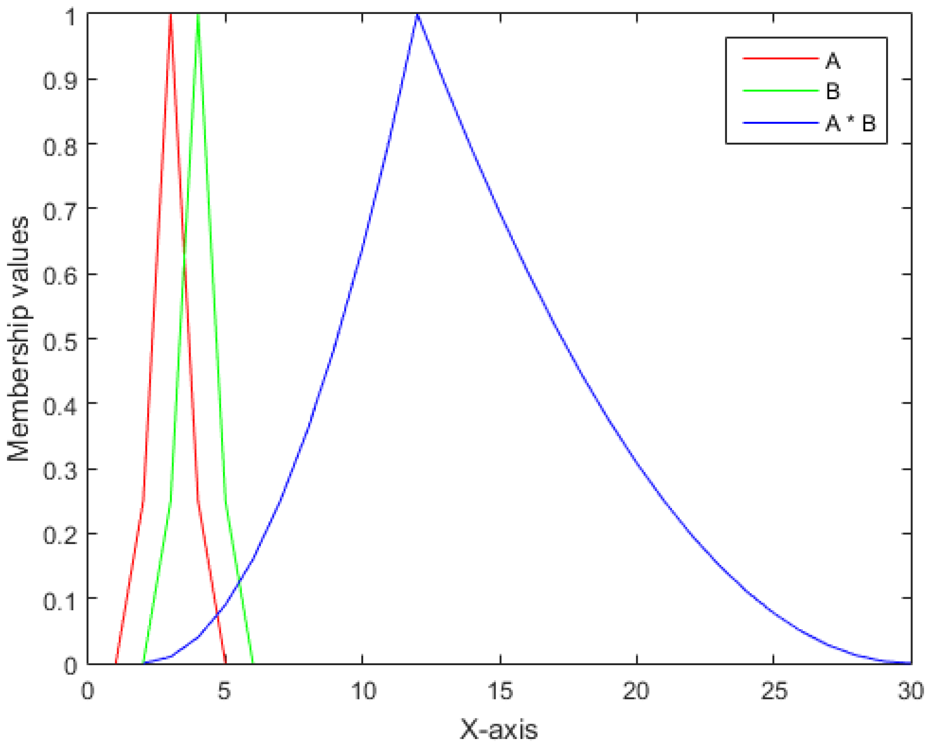
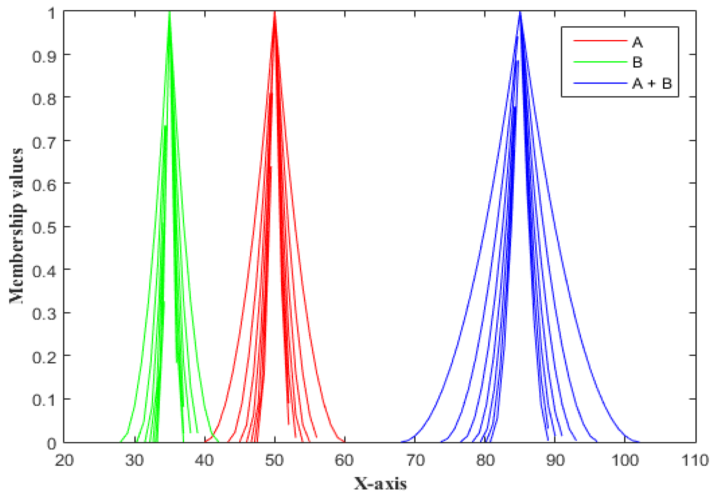
3. Arithmetic Operation over Parabolic Dense Fuzzy Numbers

Let $\widetilde{A }=\langle a\left(1-\frac{\rho }{1+n}\right), a,a\left(1+\frac{\sigma }{1+n}\right)\rangle$ and $\widetilde{B }=\langle b\left(1-\frac{{\rho }^{\prime }}{1+n}\right), b,b\left(1+\frac{{\sigma }^{\prime }}{1+n}\right)\rangle$ be two parabolic dense fuzzy numbers whose membership functions are given by

$${\mu }_{\tilde{A}}\left(x\right)=\{\begin{array}{c}{\left\{\frac{x-a\left(1-\frac{\rho }{1+n}\right)}{\frac{a\rho }{1+n}}\right\}}^2, for a\left(1-\frac{\rho }{1+n}\right)\le x\le a\hfill \\ \begin{array}{c}{\left\{\frac{a\left(1+\frac{\sigma }{1+n}\right)-x}{\frac{a\sigma }{1+n}}\right\}}^2, for a\le x\le a\left(1+\frac{\sigma }{1+n}\right)\hfill \\ 0, for x<a\left(1-\frac{\rho }{1+n}\right) or a\left(1+\frac{\sigma }{1+n}\right)<x\hfill \end{array}\hfill \end{array}$$

(6)

and

$${\mu }_{\tilde{B}}\left(y\right)=\{\begin{array}{c}{\left\{\frac{y-b\left(1-\frac{{\rho }^{\prime }}{1+n}\right)}{\frac{b{\rho }^{\prime }}{1+n}}\right\}}^2, for b\left(1-\frac{{\rho }^{\prime }}{1+n}\right)\le y\le b\hfill \\ \begin{array}{c}{\left\{\frac{b\left(1+\frac{{\sigma }^{\prime }}{1+n}\right)-y}{\frac{b{\sigma }^{\prime }}{1+n}}\right\}}^2, for b\le y\le b\left(1+\frac{{\sigma }^{\prime }}{1+n}\right)\hfill \\ 0, for y<b\left(1-\frac{{\rho }^{\prime }}{1+n}\right) or b\left(1+\frac{{\sigma }^{\prime }}{1+n}\right)<y\hfill \end{array}\hfill \end{array}$$

(7)

Here $, \sigma ,$ ${\rho }^{\prime }$, and ${\sigma }^{\prime }$ are fuzzy deviation parameters. The values of all the fuzzy deviation parameters lie within $\left(0, 1\right).$ Now, we define some basic arithmetic operations over parabolic dense fuzzy numbers according to the extension of Garg and Ansha [11], as given below.

(i)

Addition of Two Parabolic Dense Fuzzy Numbers

Let us consider two parabolic dense fuzzy numbers $\widetilde{A }$ and $\widetilde{B }$ whose membership functions are given in Equations (6) and (7). Then, the addition of these two fuzzy numbers, i.e., the fuzzy variable $\tilde{C}=\widetilde{A }+\widetilde{B,}$ is also a parabolic dense fuzzy number, and the corresponding membership function is given by

$${\mu }_{\tilde{C}}(z)=\{\begin{array}{c}{\left\{\frac{z-a\left(1-\frac{\rho }{1+n}\right)-b\left(1-\frac{{\rho }^{\prime }}{1+n}\right)}{\frac{a\rho }{1+n}+\frac{b{\rho }^{\prime }}{1+n}}\right\}}^2, for a\left(1-\frac{\rho }{1+n}\right)+b\left(1-\frac{{\rho }^{\prime }}{1+n}\right)\le z\le a+b\hfill \\ \begin{array}{c}{\left\{\frac{a\left(1+\frac{\sigma }{1+n}\right)+b\left(1+\frac{{\sigma }^{\prime }}{1+n}\right)-z}{\frac{a\sigma }{1+n}+\frac{b{\sigma }^{\prime }}{1+n}}\right\}}^2, for a+b\le z\le a\left(1+\frac{\sigma }{1+n}\right)+b\left(1+\frac{{\sigma }^{\prime }}{1+n}\right)\hfill \\ 0 , for z< a\left(1-\frac{\rho }{1+n}\right)+b\left(1-\frac{{\rho }^{\prime }}{1+n}\right) or z>a\left(1+\frac{\sigma }{1+n}\right)+b\left(1+\frac{{\sigma }^{\prime }}{1+n}\right)\hfill \end{array}\hfill \end{array}$$

(8)

Graphically, the addition of two PDFNs is given in Figure 3.

(ii)

Subtraction of Two Parabolic Dense Fuzzy Numbers

Let us consider two parabolic dense fuzzy numbers $\widetilde{A }$ and $\tilde{B}$ whose membership functions are given in Equations (6) and (7). Then, the subtraction of these two fuzzy numbers, i.e., the fuzzy variable $\tilde{C}=\widetilde{A }-\tilde{B},$ is also a parabolic dense fuzzy number, and the corresponding membership function is given by

$${\mu }_{\tilde{C}}\left(z\right)=\{\begin{array}{c}{\left\{\frac{z-a\left(1- \frac{\rho }{1+n}\right)+b\left(1+\frac{{\sigma }^{\prime }}{1+n}\right)}{\frac{a\rho }{1+n}+\frac{b{\sigma }^{\prime }}{1+n}}\right\}}^2, for a\left(1-\frac{\rho }{1+n}\right)-b\left(1+\frac{{\sigma }^{\prime }}{1+n}\right)\le z\le a-b\hfill \\ \begin{array}{c}{\left\{\frac{a\left(1+\frac{\sigma }{1+n}\right)-b\left(1-\frac{{\rho }^{\prime }}{1+n}\right)-z}{\frac{a\sigma }{1+n}+\frac{b{\rho }^{\prime }}{1+n}}\right\}}^2, for a-b\le z\le a\left(1+\frac{\sigma }{1+n}\right)-b\left(1- \frac{{\rho }^{\prime }}{1+n}\right)\hfill \\ 0, for z<a\left(1-\frac{\rho }{1+n}\right)-b\left(1+\frac{{\sigma }^{\prime }}{1+n}\right) or z>a\left(1+\frac{\sigma }{1+n}\right)-b\left(1- \frac{{\rho }^{\prime }}{1+n}\right)\end{array}\hfill \end{array}$$

(9)

Graphically, the subtraction of two PDFNs is given in Figure 4.

(iii)

Scalar multiplication of Parabolic Dense Fuzzy Numbers

Let $\tilde{A}=a\left(1-\frac{\rho }{1+n}\right), a,a\left(1+\frac{\sigma }{1+n}\right)$ be a PDFN with the membership function given in Equation (6) and $z=kx$ be the transformation; then, $k\tilde{A}$ is also a PDFN given by

$$k\tilde{A}=\{\begin{array}{c}\langle ka\left(1-\frac{\rho }{1+n}\right), ka,ka\left(1+\frac{\sigma }{1+n}\right)\rangle if k>0\\ \langle ka\left(1+\frac{\sigma }{1+n}\right),ka, ka\left(1-\frac{\rho }{1+n}\right)\rangle if k<0\end{array}$$

(10)

Graphically, the scalar multiplication of two PDFNs is given in Figure 5.

(iv)

Multiplication of Two Parabolic Dense Fuzzy Numbers

Let us consider two parabolic dense fuzzy numbers $\widetilde{A }$ and $\tilde{B}$ whose membership functions are given in Equations (6) and (7). Then, the multiplication of these two fuzzy numbers, i.e., the fuzzy variable $\tilde{C}=\widetilde{A }·\widetilde{B,}$ is also a PDFN and the corresponding membership function is given by

$${\mu }_{\widetilde{A }.\widetilde{B }}\left(z\right)=\{\begin{array}{c}{\left\{\frac{-Q_1+\sqrt{Q_1^2-4P_1\left(R_1-z\right)}}{2P_1}\right\}}^2, for a\left(1-\frac{\rho }{1+n}\right)b\left(1-\frac{{\rho }^{\prime }}{1+n}\right)\le z\le ab\hfill \\ \begin{array}{c}{\left\{\frac{-Q_2+\sqrt{Q_2^2-4P_2\left(R_2-z\right)}}{2P_2}\right\}}^2, for ab\le z\le a\left(1+\frac{\sigma }{1+n}\right)b\left(1+\frac{{\sigma }^{\prime }}{1+n}\right)\hfill \\ 0, for z<a\left(1-\frac{\rho }{1+n}\right)b\left(1-\frac{{\rho }^{\prime }}{1+n}\right) or z>a\left(1+\frac{\sigma }{1+n}\right)b\left(1+\frac{{\sigma }^{\prime }}{1+n}\right)\hfill \end{array}\end{array}$$

(11)

where $P_1=\frac{ab\rho {\rho }^1}{{\left(1+n\right)}^2}$, $Q_1=\frac{ab}{1+n}\left[\left(1-\frac{\rho }{1+n}\right){\rho }^{\prime }+\left(1-\frac{{\rho }^{\prime }}{1+n}\right)\rho \right]$, $R_1=ab\left(1-\frac{\rho }{1+n}\right)\left(1-\frac{{\rho }^{\prime }}{1+n}\right)$, $P_2=\frac{ab\sigma {\sigma }^1}{{\left(1+n\right)}^2}$, $Q_2=-\frac{ab}{1+n}\left[\left(1+\frac{\sigma }{1+n}\right){\sigma }^{\prime }+\left(1+\frac{{\sigma }^{\prime }}{1+n}\right)\sigma \right]$, and $R_2=ab\left(1+\frac{\sigma }{1+n}\right)\left(1+\frac{{\sigma }^{\prime }}{1+n}\right)$.

Graphically, the multiplication of two PDFNs is given in Figure 6.

(v)

Inverse of a Parabolic Dense Fuzzy Number

Let $\widetilde{A }$ be a parabolic dense fuzzy number whose membership function is given in Equation (6). Then, the inverse of $\widetilde{A }$, i.e., ${\tilde{A}}^{-1}=\langle a^{-1}{\left(1+\frac{\sigma }{1+n}\right)}^{-1}, a^{-1}, a^{-1}{\left(1-\frac{\rho }{1+n}\right)}^{-1}\rangle$, is also a parabolic dense fuzzy number whose membership function is

$${\mu }_{{\tilde{A}}^{-1}}\left(z\right)=\{\begin{array}{c}{\left\{\frac{za\left(1+\frac{\sigma }{1+n}\right)-1}{\frac{za\sigma }{1+n}}\right\}}^2, for a^{-1}{\left(1-\frac{\sigma }{1+n}\right)}^{-1}\le z\le a^{-1}\hfill \\ \begin{array}{c}{\left\{\frac{1-a\left(1+\frac{\rho }{1+n}\right)z}{\frac{za\rho }{1+n}}\right\}}^2, for a^{-1}\le z\le a^{-1}{\left(1+\frac{\rho }{1+n}\right)}^{-1}\hfill \\ 0 , for z< a^{-1}{\left(1-\frac{\sigma }{1+n}\right)}^{-1} or z>a^{-1}{\left(1+\frac{\rho }{1+n}\right)}^{-1}\hfill \end{array}\hfill \end{array}$$

(12)

4. Formulation of Crisp Model

Here, we considered an inventory system of fishery culture. The fishery culture in a lake was mainly assumed for our proposed model. Here, for simplification of our study, all stages of fishery culture were not considered. We considered only from the stage where the fingerlings are brought from the market and fed to reach the ideal size for customer demand. Additional assumptions of the proposed model are given below.

(i)

We considered an additional cost for feeding the growing items.

(ii)

Feeding cost depended on the weight of the items.

(iii)

The growth function was approximated by a linear function.

(iv)

We considered an idle cost for the growth period and cleaning period.

A schematic overview of the proposed model is given in Figure 7.

In Figure 8, y is the number of purchased items and g is the growth rate per fish per unit time. The initial approximate weight of each fingerling is $v_0$ and final approximate weight (at the time of selling) of each fish is $v_1$. At the beginning, $t_1$ is the time required to clean the pond, and then the fingerlings are grown up during the time $t_2$. After that, the fish are sold on the market during time $t_3$. According to this consideration, the following equations are obtained:

$$\mathrm{The} \mathrm{total} \mathrm{initial} \mathrm{weight} \mathrm{of} \mathrm{fingerlings} \mathrm{is} q_0=y{v}_0.$$

(13)

$$\mathrm{The} \mathrm{total} \mathrm{final} \mathrm{weight} \mathrm{of} \mathrm{the} \mathrm{fishes} \mathrm{is}{q}_1=y{v}_1.$$

(14)

$$t_2=\frac{q_1-q_0}{yg}=\frac{v_1-v_0}{g}.$$

(15)

$$t_3=\frac{q_1}{d}=\frac{y{v}_1}{d}.$$

(16)

$$\mathrm{Cycle} \mathrm{time} T=t_1+t_2+t_3.$$

(17)

The main objective of this proposed model is to minimize the total cost (Z) per cycle, which includes the purchasing cost, holding cost, food procurement cost (FPC), operational cost (OC), and natural idle cost (NIC).

$$Z=\mathrm{purchasing} \cos \mathrm{t}+ \mathrm{holding} \cos \mathrm{t}+ \mathrm{food} \mathrm{procurement} \cos \mathrm{t}+ \mathrm{operational} \cos \mathrm{t}+ \mathrm{natural} \mathrm{idle} \cos \mathrm{t},$$

(18)

where purchasing cost $=sy{v}_0=\frac{s{v}_{0}d{t}_3}{v_1}$, holding cost $=c_{2}T$, food procurement cost $=\frac{f{t}_2\left(q_1-q_0\right)}{2}=\frac{fd{t}_3{\left(v_1-v_0\right)}^2}{2g{v}_1}$, $\mathrm{natural} \mathrm{idle} \cos \mathrm{t} =n_c\left(t_1+t_2\right)$, and $\mathrm{operational} \cos \mathrm{t}=B$.

Putting these cost values into Equation (18) yields the total inventory cost per cycle as follows:

$$\begin{array}{l}Z=\frac{s{v}_{0}d{t}_3}{v_1}+c_{2}T+\frac{fd{t}_3{\left(v_1-v_0\right)}^2}{2g{v}_1}+n_c\left(t_1+t_2\right)+B,\\ =d\left\{\frac{s{v}_0{t}_3}{v_1}+\frac{f{t}_3{\left(v_1-v_0\right)}^2}{2g{v}_1}\right\}+\left\{c_{2}T+n_c\left(t_1+t_2\right)+B\right\},\\ =d\phi +\psi ,\end{array}$$

(19)

where,

$$\{\begin{array}{l}\phi =\frac{s{v}_0{t}_3}{v_1}+\frac{f{t}_3{\left(v_1-v_0\right)}^2}{2g{v}_1}\\ \psi =c_{2}T+n_c\left(t_1+t_2\right)+B\end{array}$$

(20)

Thus, the crisp problem is given by

$$Minimize Z=d\phi +\psi ,$$

(21)

subject to the conditions in Equations (13)–(17) and (20).

5. Fuzzy Mathematical Model

We know that the demand rate is a crucial part of any inventory problem, and it does not remain constant every time. Thus, we considered the demand rate as flexible throughout the proposed model, where it could be assumed as a parabolic dense fuzzy set. Hence, the objective function of the crisp model becomes

$$\tilde{Z}=\tilde{d}\phi +\psi ,$$

(22)

where $\phi \mathrm{and} \psi$ are given in Equation (20).

The membership functions of the parabolic dense fuzzy demand rate with n learning frequency are given by

$$\mu \left(\tilde{d}\right)=\{\begin{array}{c}{\left\{\frac{x-d\left(1-\frac{\rho }{1+n}\right)}{\frac{d\rho }{1+n}}\right\}}^2, for d\left(1-\frac{\rho }{1+n}\right)\le x\le d\hfill \\ \begin{array}{c}{\left\{\frac{d\left(1+\frac{\sigma }{1+n}\right)-x}{\frac{d\sigma }{1+n}}\right\}}^2, for d\le x\le d\left(1+\frac{\sigma }{1+n}\right)\hfill \\ 0, for x<d\left(1-\frac{\rho }{1+n}\right) or x>d\left(1+\frac{\sigma }{1+n}\right)\hfill \end{array}\hfill \end{array}$$

(23)

The left and right $\alpha$-cuts of the above membership function are given by

$$\left[{\mu }_L^d,{\mu }_R^d\right]=\left[d+\frac{d\rho \left(\sqrt{\alpha }-1\right)}{1+n}, d+\frac{d\sigma \left(1-\sqrt{\alpha }\right)}{1+n}\right].$$

(24)

Then, the index value of the demand rate is given by

$$\begin{array}{cc}I\left(\tilde{d}\right)& =\frac{1}{2N}{\displaystyle {\displaystyle \sum }_{n=1}^N}\underset{\alpha =0}{\overset{1}{{\displaystyle \int }}}\left\{d+\frac{d\rho \left(\sqrt{\alpha }-1\right)}{1+n}+d+\frac{d\sigma \left(1-\sqrt{\alpha }\right)}{1+n}\right\}d\alpha ,\\ & =\frac{1}{2N}{\displaystyle {\displaystyle \sum }_{n=1}^N}\left\{2d+\frac{2d\left(\rho -\sigma \right)}{3\left(1+n\right)}+\frac{d\left(\sigma -\rho \right)}{1+n}\right\},\hfill \\ & =d+\frac{d\left(\sigma -\rho \right)}{6N}\left\{\frac{1}{2}+\frac{1}{3}+\dots +\frac{1}{N}\right\}.\hfill \end{array}$$

(25)

Again, the equation

$Z=d\phi +\psi$ can be rewritten as

$$d=\frac{Z-\psi }{\phi }.$$

(26)

Substituting Equation (26) into Equation (23), we obtain the membership function of the objective function as follows:

$$\mu \left(\widetilde{Z }\right)=\{\begin{array}{c}{\left\{\frac{\frac{Z-\psi }{\phi }-d\left(1-\frac{\rho }{1+n}\right)}{\frac{d\rho }{1+n}}\right\}}^2, for d\phi \left(1-\frac{\rho }{1+n}\right)+\psi \le x\le d\phi +\psi \\ \begin{array}{c}{\left\{\frac{d\left(1+\frac{\sigma }{1+n}\right)-\frac{Z-\psi }{\phi }}{\frac{d\sigma }{1+n}}\right\}}^2, for d\phi +\psi \le x\le d\phi \left(1+\frac{\sigma }{1+n}\right)+\psi \\ 0, for x<d\phi \left(1-\frac{\rho }{1+n}\right)+\psi or x>d\phi \left(1+\frac{\sigma }{1+n}\right)+\psi \end{array}\end{array}$$

(27)

The left and right $\alpha$-cuts of the above membership function are given by

$$\left[{\mu }_L^d,{\mu }_R^d\right]=\left[d\phi +\psi +\frac{d\rho \phi \left(\sqrt{\alpha }-1\right)}{1+n}, d\phi +\psi +\frac{d\sigma \phi \left(1-\sqrt{\alpha }\right)}{1+n}\right].$$

(28)

Then, the index value of the fuzzy objective function is given by

$$\begin{array}{l}I\left(\tilde{Z}\right)=\frac{1}{2N}{\displaystyle {\displaystyle \sum }_{n=1}^N}\underset{\alpha =0}{\overset{1}{{\displaystyle \int }}}\left\{d\phi +\psi +\frac{d\rho \phi \left(\sqrt{\alpha }-1\right)}{1+n}+d\phi +\psi +\frac{d\sigma \phi \left(1-\sqrt{\alpha }\right)}{1+n}\right\}d\alpha ,\\ =\frac{1}{2N}{\displaystyle {\displaystyle \sum }_{n=1}^N}\left\{2\left(d\phi +\psi \right)+\frac{2d\phi \left(\rho -\sigma \right)}{3\left(1+n\right)}+\frac{d\phi \left(\sigma -\rho \right)}{1+n}\right\},\\ =d\phi +\psi +\frac{d\phi \left(\sigma -\rho \right)}{6N}\left\{\frac{1}{2}+\frac{1}{3}+\dots +\frac{1}{N}\right\}.\end{array}$$

(29)

Thus, the problem under a parabolic dense fuzzy approach becomes

$$\{\begin{array}{c}Maximize I\left(\tilde{Z}\right)=d\phi +\psi +\frac{d\phi \left(\sigma -\rho \right)}{6N}\left\{\frac{1}{2}+\frac{1}{3}+\dots +\frac{1}{N}\right\}\\ I\left(\tilde{d}\right)=d+\frac{d\left(\sigma -\rho \right)}{6N}\left\{\frac{1}{2}+\frac{1}{3}+\dots +\frac{1}{N}\right\} \\ Subject to condition \left(13\right)–\left(17\right) \mathrm{and} \left(20\right)\end{array}$$

(30)

Next, we considered the demand rate as a parabolic dense fuzzy lock set, where the membership function of the demand rate becomes

$$\mu \left(\tilde{d}\right)=\{\begin{array}{c}{\left\{\frac{x-d\left(1-\rho \left(\frac{1}{l_1}-\frac{1}{1+n}\right)\right)}{d\rho \left(\frac{1}{l_1}-\frac{1}{1+n}\right)}\right\}}^2, for d\left(1-\rho \left(\frac{1}{l_1}-\frac{1}{1+n}\right)\right)\le x\le d\hfill \\ \begin{array}{c}{\left\{\frac{d\left(1+\sigma \left(\frac{1}{l_2}-\frac{1}{1+n}\right)\right)-x}{d\sigma \left(\frac{1}{l_2}-\frac{1}{1+n}\right)}\right\}}^2, for d\le x\le d\left(1+\sigma \left(\frac{1}{l_2}-\frac{1}{1+n}\right)\right)\hfill \\ 0, for x<d\left(1-\rho \left(\frac{1}{l_1}-\frac{1}{1+n}\right)\right) or x>d\left(1+\sigma \left(\frac{1}{l_2}-\frac{1}{1+n}\right)\right)\hfill \end{array}\hfill \end{array}$$

(31)

The left and right $\alpha$-cuts of the above membership function are given by

$$\left[{\mu }_L^d,{\mu }_R^d\right]=\left[d+d\rho \left(\sqrt{\alpha }-1\right)\left(\frac{1}{l_1}-\frac{1}{1+n}\right),d+d\sigma \left(1-\sqrt{\alpha }\right)\left(\frac{1}{l_2}-\frac{1}{1+n}\right)\right].$$

(32)

Thus, the index value of demand rate is given by

$$\begin{array}{cc}I\left(\tilde{d}\right)& =\frac{1}{2N}{\displaystyle {\displaystyle \sum }_{n=1}^N}\underset{\alpha =0}{\overset{1}{{\displaystyle \int }}}\left\{{\mu }_L^d+{\mu }_R^d\right\}d\alpha ,\hfill \\ & =\frac{1}{2N}{\displaystyle {\displaystyle \sum }_{n=1}^N}\underset{\alpha =0}{\overset{1}{{\displaystyle \int }}}\left\{d+d\rho \left(\sqrt{\alpha }-1\right)\left(\frac{1}{l_1}-\frac{1}{1+n}\right)+d+d\sigma \left(1-\sqrt{\alpha }\right)\left(\frac{1}{l_2}-\frac{1}{1+n}\right)\right\}d\alpha ,\hfill \\ & =\frac{1}{2N}{\displaystyle {\displaystyle \sum }_{n=1}^N}\left\{2d+\frac{2d\sigma }{3}\left(\frac{1}{l_2}-\frac{1}{1+n}\right)-\frac{2d\rho }{3}\left(\frac{1}{l_1}-\frac{1}{1+n}\right)\right\},\hfill \\ & =d+\frac{d}{3}\left(\frac{\sigma }{l_2}-\frac{\rho }{l_1}\right)+\frac{d\left(\rho -\sigma \right)}{3N}\left\{\frac{1}{2}+\frac{1}{3}+\dots +\frac{1}{N}\right\}.\hfill \end{array}$$

(33)

Then, substituting Equation (26) into Equation (31), we obtain the membership function of the fuzzy objective function as given below.

$$\mu \left(\tilde{Z}\right)=\{\begin{array}{c}{\left\{\frac{\frac{z-\psi }{\phi }-d\left(1-\rho \left(\frac{1}{l_1}-\frac{1}{1+n}\right)\right)}{d\rho \left(\frac{1}{l_1}-\frac{1}{1+n}\right)}\right\}}^2, for d\phi \left(1-\rho \left(\frac{1}{l_1}-\frac{1}{1+n}\right)\right)+\psi \le z\le d\phi +\psi \hfill \\ \begin{array}{c}{\left\{\frac{d\left(1+\sigma \left(\frac{1}{l_2}-\frac{1}{1+n}\right)\right)-\frac{z-\psi }{\phi }}{d\sigma \left(\frac{1}{l_2}-\frac{1}{1+n}\right)}\right\}}^2, for d\phi +\psi \le z\le d\phi \left(1+\sigma \left(\frac{1}{l_2}-\frac{1}{1+n}\right)\right)+\psi \hfill \\ 0, for x<d\phi \left(1-\rho \left(\frac{1}{l_1}-\frac{1}{1+n}\right)\right)+\psi or x>d\phi \left(1+\sigma \left(\frac{1}{l_2}-\frac{1}{1+n}\right)\right)+\psi \hfill \end{array}\hfill \end{array}$$

(34)

The left and right $\alpha$-cuts of the above membership function are given by

$$\left[{\mu }_L^d,{\mu }_R^d\right]=\left[d\phi +\psi +d\phi \rho \left(\sqrt{\alpha }-1\right)\left(\frac{1}{l_1}-\frac{1}{1+n}\right),d\phi +\psi +d\phi \sigma \left(1-\sqrt{\alpha }\right)\left(\frac{1}{l_2}-\frac{1}{1+n}\right)\right].$$

(35)

Then, the index value of the fuzzy objective function is given by

$$\begin{array}{cc}I\left(\tilde{Z}\right)& =\frac{1}{2N}{\displaystyle {\displaystyle \sum }_{n=1}^N}{\displaystyle \underset{\alpha =0}{\overset{1}{{\displaystyle \int }}}}\{d\phi +\psi +d\phi \rho \left(\sqrt{\alpha }-1\right)\left(\frac{1}{l_1}-\frac{1}{1+n}\right),d\phi +\psi \hfill \\ & +d\phi \sigma \left(1-\sqrt{\alpha }\right)\left(\frac{1}{l_2}-\frac{1}{1+n}\right)\}d\alpha ,\hfill \\ & =\frac{1}{2N}{\displaystyle {\displaystyle \sum }_{n=1}^N}\left\{2\left(d\phi +\psi \right)-\frac{2d\phi \rho }{3}\left(\frac{1}{l_1}-\frac{1}{1+n}\right)+\frac{2d\phi \sigma }{3}\left(\frac{1}{l_2}-\frac{1}{1+n}\right)\right\},\\ & =d\phi +\psi +\frac{d\phi }{3}\left(\frac{\sigma }{l_2}-\frac{\rho }{l_1}\right)+\frac{d\phi \left(\rho -\sigma \right)}{3N}\left\{\frac{1}{2}+\frac{1}{3}+\dots +\frac{1}{N}\right\}.\hfill \end{array}$$

(36)

Thus, the problem under a PDFLS approach becomes

$$\{\begin{array}{c}Maximize I\left(\tilde{Z}\right)=d\phi +\psi +\frac{d\phi }{3}\left(\frac{\sigma }{l_2}-\frac{\rho }{l_1}\right)+\frac{d\phi \left(\rho -\sigma \right)}{3N}\left\{\frac{1}{2}+\frac{1}{3}+\dots +\frac{1}{N}\right\}\\ I\left(\tilde{d}\right)=d+\frac{d}{3}\left(\frac{\sigma }{l_2}-\frac{\rho }{l_1}\right)+\frac{d\left(\rho -\sigma \right)}{3N}\left\{\frac{1}{2}+\frac{1}{3}+\dots +\frac{1}{N}\right\} \\ Subject to condition \left(13\right)–\left(17\right) \mathrm{and} \left(20\right)\end{array}$$

(37)

If we substitute $l_1=l_2=1$ and $N\to \infty$ into Equation (37), then the TDFLS problem becomes a general fuzzy problem.

$$\{\begin{array}{c}Maximize I\left(\tilde{Z}\right)=d\phi +\psi +\frac{d\phi }{3}\left(\sigma -\rho \right)+\frac{d\phi \left(\rho -\sigma \right)}{3N}\left\{\frac{1}{2}+\frac{1}{3}+\dots +\frac{1}{N}\right\}\\ I\left(\tilde{d}\right)=d+\frac{d}{3}\left(\sigma -\rho \right)+\frac{d\left(\rho -\sigma \right)}{3N}\left\{\frac{1}{2}+\frac{1}{3}+\dots +\frac{1}{N}\right\} \\ Subject to condition \left(13\right)–\left(17\right) \mathrm{and} \left(20\right)\end{array}$$

(38)

5.1. Rules of Finding Key Values of the Fuzzy Locks

Every fuzzy parameter has two bounds, namely, an upper bound ($b^U,$ if known) and a lower bound ($b^L,$ if known) or both. For a single key, if the upper bound is known, then the index value of $\tilde{b}$ is given by $I\left(\tilde{b}\right)\le b^U$, which implies $k\ge \frac{b\left(\sigma -\rho \right)}{4\left(b^U-b\right)}$. If the lower bound is given, then $I\left(\tilde{b}\right)\ge b^L$ implies $k\ge \frac{b\left(\rho -\sigma \right)}{4\left(b-b^L\right)}$. For double keys, the index value of $\widetilde{A }$ is given by

$$I\left(\tilde{B}\right)=\frac{1}{2N}{\displaystyle {\displaystyle \sum }_{n=0}^N}\underset{0}{\overset{1}{{\displaystyle \int }}}\left\{{\mu }_L^B+{\mu }_R^B\right\}d\alpha =\frac{b}{2}\left(1-\frac{\rho }{2l_1}\right)+\frac{b}{2}\left(1+\frac{\sigma }{2l_2}\right).$$

(39)

Thus,

$$\frac{b}{2}\left(1-\frac{\rho }{2l_1}\right)\ge b^L\Rightarrow l_1\ge \frac{b\rho }{2\left(b-2b^L\right)} \mathrm{and} \frac{b}{2}\left(1+\frac{\sigma }{2l_2}\right)\le b^U\Rightarrow l_2\ge \frac{b\sigma }{2\left(2b^U-b\right)}.$$

(40)

5.2. Solution Algorithm

The solution algorithm of our proposed model is given below.

Input: Values of all parameters $(d, g$, $v_0$, $v_1$, $t_1$, $s$, $f$, $c_2$, $n_c$, $B$,

$l_1,l_2,\rho \mathrm{and} \sigma )$.

Output: The optimum inventory cost of the proposed model.

Step 1. Solve the problem in a crisp sense first using Equation (21).

Step 2. Consider demand as a parabolic dense fuzzy number.

Step 3. Find the index value of the inventory cost function in PDFS approach using Equation (30).

Step 4. Consider demand as a parabolic dense fuzzy lock set.

Step 5. Find the corresponding inventory cost using Equation (37).

Step 6. Compare among crisp, general fuzzy, PDFS, and PDFLS results and obtain the minimum inventory cost of the proposed model.

Step 7. End.

6. A Real Case Study

We visited the West Bengal fisheries corporation Ltd. situated in Sector V, Salt Lake City, Kolkata, West Bengal 700091, India ((latitude, longitude) = (22.5691° N, 88.4337° E)) on 10 December 2020. After a long discussion with the manager Mr. Mukherjee, we knew that they cleaned the lake properly at the beginning of each cycle. After that, the fingerlings were stocked and fed in the lake until the fingerlings acquired the ideal size for selling. We collected some valuable data related to our proposed model: $d=\mathrm{4,000,000} \mathrm{g}/\mathrm{year}, g=912.5$ g/year, $v_0=100$ g,

$v_1=600$ g,

$t_1=0.019$ year, $s=\$0.01$ g, $f=\$0.8$/g/year, $c_2=\$100$/year, $n_c=\$40$/year, $B=\$80$/year, $\rho =0.4, \mathrm{and} \sigma =0.2$. The upper bound and lower bound of the demand rate were set to $d_0^L=\mathrm{3,600,000} \mathrm{and} d_0^U=\mathrm{4,000,000}$. Utilising the above rule, the key values of the demand rate were obtained as follows:

$$\left[\begin{array}{c}{l}_1\\ l_2\end{array}\right]\ge \left[\begin{array}{c}\frac{d\rho }{2\left(d-2d^L\right)}\\ \frac{d\sigma }{2\left(2d^U-d\right)}\end{array}\right]=\left[\begin{array}{c}\frac{\mathrm{4,000,000}\times 0.4}{2\left(\mathrm{4,000,000}-2\times \mathrm{3,600,000}\right)}\\ \frac{\mathrm{4,000,000}\times 0.2}{2\left(2\times \mathrm{4,400,000}-\mathrm{4,000,000}\right)}\end{array}\right]=\left[\begin{array}{c}-0.25\\ 0.083\end{array}\right].$$

(41)

Satisfying the above condition, let $l_1=0.38 \mathrm{and} l_2=0.25$; accordingly, the optimal solutions of the crisp model and several fuzzy models are given in

Table 2. Numerical result of the proposed model.

Approach	${\mathit{N}}^{*}$	$\mathbf{Time} \left({\mathit{t}}_2^{*}\right)$	$\mathbf{Time} \left({\mathit{t}}_3^{*}\right)$	$\mathbf{Ordered} \mathbf{Items} \left({\mathit{y}}^{*}\right)$	$\mathbf{Total} \mathbf{Cos}\mathbf{t} \left({\mathit{Z}}^{*}\right)$	$\frac{{\mathit{Z}}^{*}-{\mathit{Z}}_{\mathit{C}\mathit{r}\mathit{i}\mathit{s}\mathit{p}}^{*}}{{\mathit{Z}}_{\mathit{C}\mathit{r}\mathit{i}\mathit{s}\mathit{p}}^{*}}\times 100$
Crisp	-	0.5479	0.4330	2887	319,476.8	-
General Fuzzy	-	0.5479	0.4330	2790	308,834.3	−3.33
Parabolic dense fuzzy	1	0.5479	0.4327	2838	314,155.5	−1.66
	2	0.5479	0.4321	2846	315,042.4	−1.39
	3	0.5479	0.4318	2852	315,633.7	−1.20
PDFLS	1	05479	0.4330	2740	303,233.0	−5.08
	2	0.5479	0.4331	2724	301,459.3	−5.64
	3	0.5479	0.4330	2713	300,276.8	−6.00

.

Table 2 shows that the total inventory cost of the proposed model is $319,476.8 in the crisp case. For a general fuzzy environment, the inventory cost is $308,834.3. In a parabolic dense fuzzy environment, the minimum total inventory cost is $314,155.5 for learning experience N = 1, whereas, for TDFLS, the minimum total inventory cost is $300,276.8 with a growing period of 0.5479 years ≈ 200 days, a selling period of 0.4327 years ≈ 158 days, and 2838 ordered items for learning experience N = 3. From Table 2, it is also clear that, in the general fuzzy model, the total inventory cost decreases by 3.33%. In the parabolic dense fuzzy model, the total inventory cost decreases by 1.66%, whereas, in the PDFLS model, the total inventory cost decreases by 6.00%. Thus, TDFLS gave the minimum inventory cost of the proposed model.

Sensitivity Analysis

From Table 2, we can see that parabolic dense fuzzy lock set gave the optimum value of the proposed model. Hence, we conducted a sensitivity analysis over the parabolic dense fuzzy model. We changed each parameter $\left(v_0,v_1,s,f,c_2,n_c,\rho , \mathrm{and} \sigma \right)$ from −30% to +30%, and the results are given in

Table 3. Sensitivity analysis of the parabolic dense fuzzy model.

Parameter	% Change	$\mathbf{Time} \left({\mathit{t}}_2^{*}\right)$	$\mathbf{Time} \left({\mathit{t}}_3^{*}\right)$	$\mathbf{Ordered} \mathbf{Items} \left({\mathit{y}}^{*}\right)$	$\mathbf{Total} \mathbf{Cos}\mathbf{t} \left({\mathit{Z}}^{*}\right)$	$\frac{{\mathit{Z}}^{*}-{\mathit{Z}}_{\mathit{C}\mathit{r}\mathit{i}\mathit{s}\mathit{p}}^{*}}{{\mathit{Z}}_{\mathit{C}\mathit{r}\mathit{i}\mathit{s}\mathit{p}}^{*}}\times 100$
$v_0$	+30	0.5151	0.4659	2919	286,691.8	−10.26
	+10	0.5369	0.4440	2782	296,074.7	−7.32
	−10	0.5589	0.4220	2644	304,128.4	−4.80
	−30	0.5808	0.4002	2507	310,708.3	−2.74
$v_1$	+30	0.7452	0.2358	1136	231,708.0	−27.47
	+10	0.6137	0.3673	2092	289,909.2	−9.25
	−10	0.4822	0.4988	3472	298,384.2	−6.60
	−30	0.3507	0.6303	5642	259,093.1	−18.90
$s$	+30	0.5479	0.4330	2713	301,090.8	−5.75
	+10	0.5479	0.4330	2713	300,548.1	−5.92
	−10	0.5479	0.4330	2713	300,005.4	−6.09
	−30	0.5479	0.4330	2713	299,462.7	−6.26
$f$	+30	0.5479	0.4330	2713	389,485.0	+21.91
	+10	0.5479	0.4330	2713	330,012.8	+3.29
	−10	0.5479	0.4330	2713	270,540.7	−15.31
	−30	0.5479	0.4330	2713	211,068.6	−33.93
$c_2$	+30	0.5479	0.4330	2713	300,306.8	−6.00
	+10	0.5479	0.4330	2713	300,286.3	−6.00
	−10	0.5479	0.4330	2713	300,266.8	−6.01
	−30	0.5479	0.4330	2713	300,246.8	−6.01
$n_c$	+30	0.5479	0.4330	2713	300,283.6	−6.00
	+10	0.5479	0.4330	2713	300,279.0	−6.00
	−10	0.5479	0.4330	2713	300,274.5	−6.01
	−30	0.5479	0.4330	2713	300,270.0	−6.01
$\rho$	+30	0.5479	0.4330	2451	271,280.7	−15.08
	+10	0.5479	0.4330	2626	290,611.4	−9.03
	−10	0.5479	0.4330	2800	309,942.1	−2.98
	−30	0.5479	0.4330	2975	329,272.8	+3.06
$\sigma$	+30	0.5479	0.4330	2923	323,512.8	+1.26
	+10	0.5479	0.4330	2783	308,022.1	−3.58
	−10	0.5479	0.4330	2643	292,531.4	−8.43
	−30	0.5479	0.4330	2503	277,040.7	−13.28

. Furthermore, a graphical illustration of Table 3 is presented in Section 7.

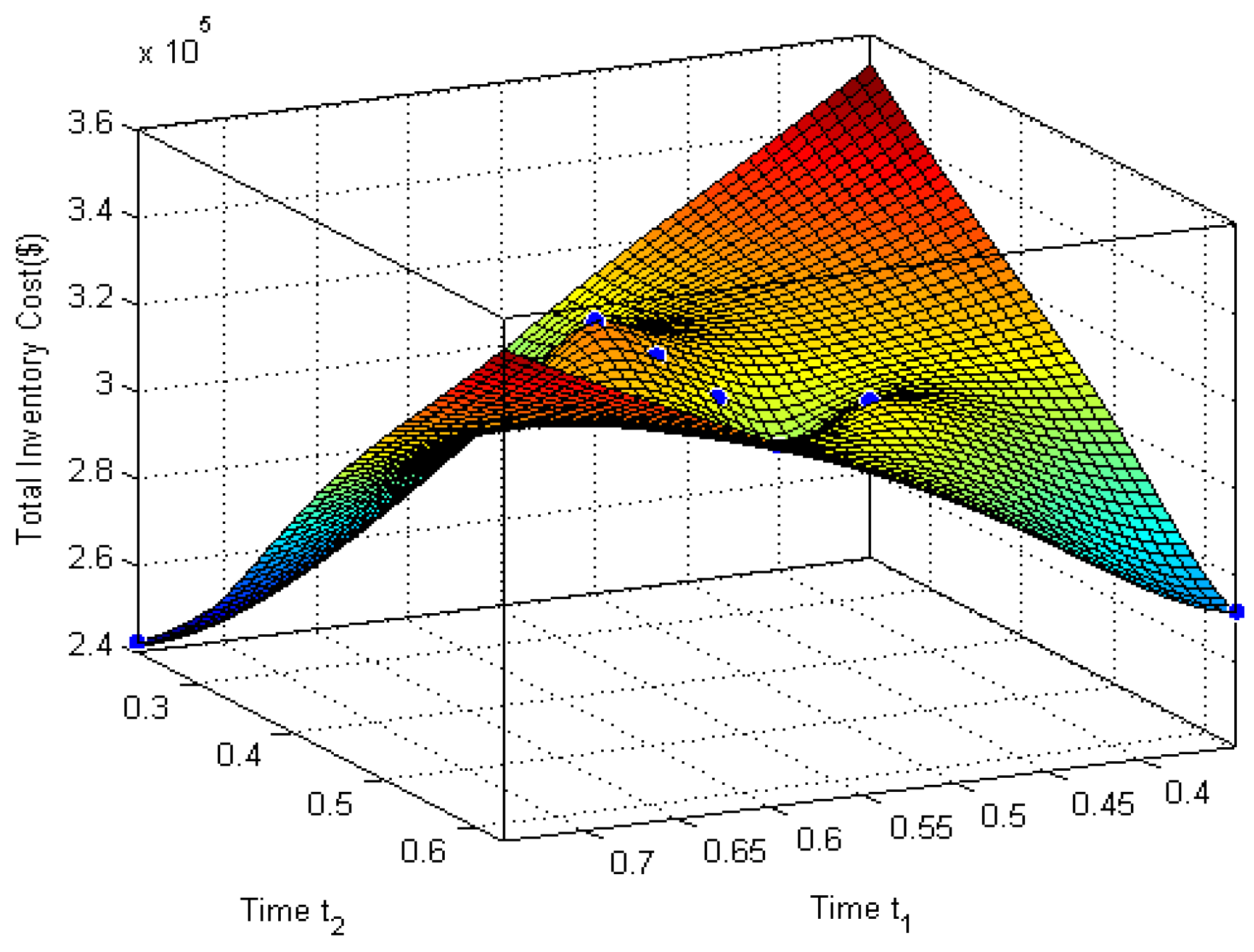
7. Graphical Illustration

In this section, we provide several graphs (Figure 9, Figure 10, Figure 11, Figure 12 and Figure 13) to illustrate the numerical results in Table 2 and the sensitivity analysis results in Table 3. The figures are given below.

Figure 9 shows that the inventory cost obtains the minimum value in a PDFLS environment, whereas it obtains the maximum in a crisp sense. Moreover, the inventory cost for the general fuzzy approach assumes a lower value than the parabolic dense fuzzy approach. Thus, by applying the parabolic dense fuzzy lock set approach, the inventory practitioner can minimize the total inventory cost.

Figure 10 shows that the approximated weight of fingerlings $\left(v_0\right)$ and deviation parameter $\left(\rho , \sigma \right)$ were not very sensitive, whereas the price of fingerlings $\left(s\right)$, holding cost $\left(c_2\right)$, and natural idle cost $\left(n_c\right)$ were insensitive within this variation. However, the feeding cost $\left(f\right)$ and approximated weight of fish at the time of selling $\left(v_1\right)$ were highly sensitive parameters for this system. Thus, to minimize the inventory cost, these two parameters $\left(f,v_1\right)$ should be handled carefully.

Figure 11 shows how the total inventory cost depends on time t₁ and time t₂. From this surface figure, it is clear that, when feeding time $t_1$ increases and selling period $t_2$ decreases, the inventory cost obtains the minimum value. Moreover, when feeding time $t_1$ decreases and selling period $t_2$ increases, the inventory cost decreases. On the other hand, when both ($t_1, t_2$) increase or decrease together, the inventory cost also increases.

Figure 12 represents the relationship among ordered items, feeding time ($t_1)$, and selling period ($t_2)$. From this figure, it is clear that ordered items obtain the maximum value when the feeding time is minimum and the selling period is maximum. Furthermore, ordered items obtain the minimum value when the feeding time is maximum and the selling period is minimum.

Figure 13 illustrates the relationship between total inventory cost and ordered items. In this figure, a smooth spline curve was drawn using the data of $y^{*}$ and $Z^{*}$ from Table 3. From the above figure, it is clear that total inventory cost does not monotonically increase with respect to ordered items. Therefore, from this graphical illustration, we can easily predict the value of ordered items when the total inventory cost is supposed to obtain a minimum value.

8. Managerial Insights

In this article, we studied some basic arithmetic operations over parabolic dense fuzzy numbers. We also defined the parabolic dense fuzzy lock set and its application in inventory management. An EOQ model of fishery culture was considered as a case study. We evaluated several decision variables such as the growing period (year), selling period (year), and the number of items ordered in each period. A decision maker can solve/tackle any complex situation of an entire industry with proper insight. The basic managerial insights of our proposed model are given below.

(i)

Learning experience is a crucial part of any inventory problem to optimize the inventory cost.

(ii)

The decision maker can optimize the inventory cost by utilizing proper key values.

(iii)

The less qualified decision maker can also minimize the cost using the PDFLS approach.

(iv)

The PDFLS approach gives a finer optimum than the parabolic dense set approach.

9. Conclusions

In this paper, we defined the parabolic dense fuzzy number with some basic arithmetic operations. Here, we developed an EOQ model for fishery culture using a real case study. We assumed that a linear function could estimate the growth rate of fish. The proposed EOQ inventory model studied the fishery culture that fed fingerlings until they were ready for sale with an ideal weight for the customer. Here, natural idle cost was considered during feeding and cleaning time. The main aim of this work was to find the number of ordering items such that the total inventory cost was minimized. In the fuzzy mathematical model, the demand rate was considered as a parabolic dense fuzzy lock set. The numerical result revealed that the parabolic dense fuzzy lock model obtained the minimum cost compared with the crisp and other fuzzy models.

This model also had some limitations. This model is not applicable to experience-free enterprises or newly set up inventory systems. In this approach, adequate manpower is required to collect more information about the model.

For future research, researchers may use the PDFLS concept in various inventory problems such as supply chain management problems, transportation problems, and trade credit problems. The PDFLS concept may be incorporate into a trapezoidal fuzzy number, pentagonal fuzzy number, hexagonal fuzzy number, heptagonal fuzzy number, etc. for a more realistic approach.

References

1. Zadeh, L.A. Fuzzy sets. Inf. Control 1965, 8, 338–356. [Google Scholar] [CrossRef] [Green Version]
2. Bellman, R.E.; Zadeh, L.A. Decision making in a fuzzy environment. Manag. Sci. 1970, 17, 141–164. [Google Scholar] [CrossRef]
3. Dubois, D.; Prade, H. Operations on fuzzy numbers. Int. J. Syst. Sci. 1978, 9, 613–626. [Google Scholar] [CrossRef]
4. Atanassov, K.T. Intuitionistic fuzzy sets. In Proceedings of the VII ITKR’s Session, Sofia, Bulgaria, 20–23 June 1983. [Google Scholar]
5. Kaufmann, A.; Gupta, M.M. Introduction of Fuzzy Arithmetic Theory and Applications; Van Nostrand Reinhold: New York, NY, USA, 1985. [Google Scholar]
6. Chutia, R.; Mahanta, S.; Baruah, H.K. An Alternative Method of Finding the Membership of a Fuzzy Number. Int. J. Latest Trends Comput. 2010, 1, 69–72. [Google Scholar]
7. De, S.K.; Beg, I. Triangular dense fuzzy sets and new defuzzication methods. J. Intell. Fuzzy Syst. 2016, 36, 469–477. [Google Scholar] [CrossRef]
8. De, S.K.; Mahata, G.C. Decision of a fuzzy inventory with fuzzy backorder model under cloudy fuzzy demand rate. Int. J. Appl. Comput. Math. 2016, 3, 2593–2609. [Google Scholar] [CrossRef]
9. De, S.K. Triangular Dense Fuzzy Lock Set. Soft Comput. 2017, 22, 7243–7254. [Google Scholar] [CrossRef]
10. Faritha, A.A.; Priya, G. Optimizing triangular parabolic fuzzy EOQ model with shortage using nearest interval approximation. Int. J. Future Revolut. Comput. Sci. Commun. Eng. 2017, 3, 92–96. [Google Scholar]
11. Garg, H.; Ansha. Arithmetic operations on generalized parabolic fuzzy numbers and its application. Proc. Natl. Acad. Sci. India Sect. A Phys. Sci. 2016, 88, 15–26. [Google Scholar] [CrossRef]
12. Maity, S.; Chakraborty, A.; De, S.K.; Mondal, S.P.; Alam, S. A comprehensive study of a backlogging EOQ model with non-linear heptagonal dense fuzzy environment. RAIRO-Oper. Res. 2020, 54, 267–286. [Google Scholar] [CrossRef] [Green Version]
13. Maity, S.; De, S.K.; Mondal, S.K. A Study of a Backorder EOQ Model for Cloud-Type Intuitionistic Dense Fuzzy Demand Rate. Int. J. Fuzzy Syst. 2019, 22, 201–211. [Google Scholar] [CrossRef]
14. Harris, F.W. Operations and Costs (Factory Management Series); A. W. Shaw Co.: Chicago, IL, USA, 1913; pp. 18–52. [Google Scholar]
15. Karlin, S. One Stage Inventory Model with Uncertainty, Studies in the Mathematical Theory of Inventory and Production; Stanford University Press: Stanford, CA, USA, 1958. [Google Scholar]
16. De, S.K. EOQ model with natural idle time and wrongly measured demand rate. Int. J. Inventory Control Manag. 2013, 3, 329–354. [Google Scholar]
17. Das, P.; De, S.K.; Sana, S.S. An EOQ model for time dependent backlogging over idle time: A step order fuzzy approach. Int. J. Appl. Comput. Math. 2014, 1, 171–185. [Google Scholar] [CrossRef] [Green Version]
18. De, S.K.; Goswami, A.; Sana, S.S. An interpolating by pass to Pareto optimality in intuitionistic fuzzy technique for an EOQ model with time sensitive backlogging. Appl. Math. Comput. 2014, 230, 664–674. [Google Scholar] [CrossRef]
19. Kazemi, N.; Olugu, E.U.; Salwa Hanim, A.-R.; Ghazilla, R.A.B.R. Development of a fuzzy economic order quantity model for imperfect quality items using the learning effect on fuzzy parameters. J. Intell. Fuzzy Syst. 2015, 28, 2377–2389. [Google Scholar] [CrossRef]
20. De, S.K.; Sana, S.S. The (p, q, r, l) model for stochastic demand under intuitionistic fuzzy aggregation with Bonferroni mean. J. Intell. Manuf. 2016, 29, 1753–1771. [Google Scholar] [CrossRef]
21. Karmakar, S.; De, S.K.; Goswami, A. A pollution sensitive dense fuzzy economic production quantity model with cycle time dependent production rate. J. Clean. Prod. 2017, 154, 139–150. [Google Scholar] [CrossRef]
22. Karmakar, S.; De, S.K.; Goswami, A. A pollution sensitive remanufacturing model with waste items: Triangular dense fuzzy lock set approach. J. Clean. Prod. 2018, 187, 789–803. [Google Scholar] [CrossRef]
23. Maity, S.; De, S.K.; Pal, M. Two Decision Makers’ Single Decision over a Back Order EOQ Model with Dense Fuzzy Demand Rate. Financ. Mark. 2018, 3, 1–11. [Google Scholar]
24. Maity, S.; De, S.K.; Mondal, S.P. A Study of an EOQ Model under Lock Fuzzy Environment. Mathematics 2019, 7, 75. [Google Scholar] [CrossRef] [Green Version]
25. De, S.K.; Mahata, G.C. A cloudy fuzzy economic order quantity model for imperfect-quality items with allowable proportionate discounts. J. Ind. Eng. Int. 2019, 15, 571–583. [Google Scholar] [CrossRef] [Green Version]
26. Liang, R.; Wang, J.Q. A Linguistic Intuitionistic Cloud Decision Support Model with Sentiment Analysis for Product Selection in E-commerce. Int. J. Fuzzy Syst. 2019, 21, 963–977. [Google Scholar] [CrossRef]
27. Nobil, A.H.; Sedigh, A.H.A.; Cárdenas-Barrón, L.E. A Generalized Economic Order Quantity Inventory Model with Shortage: Case Study of a Poultry Farmer. Arab. J. Sci. Eng. 2018, 44, 2653–2663. [Google Scholar] [CrossRef]
28. Rezaei, J. Economic order quantity for growing items. Int. J. Prod. Econ. 2014, 155, 109–113. [Google Scholar] [CrossRef]
29. Zhang, Y.; Li, L.Y.; Tian, X.Q.; Feng, C. Inventory management research for growing items with carbon-constrained. In Proceedings of the Control Conference (CCC), IEEE 35th Chinese, Chengdu, China, 27–29 July 2016; pp. 9588–9593. [Google Scholar]
30. De, S.K.; Mahata, G.C.; Maity, S. Carbon emission sensitive deteriorating inventory model with trade credit under volumetric fuzzy system. Int. J. Intell. Syst. 2021, 1–28. [Google Scholar] [CrossRef]
31. Mahata, G.C.; De, S.K.; Maity, S.; Bhattacharya, K. Three-echelon supply chain model in an imperfect production system with inspection error, learning effect, and return policy under fuzzy environment. Int. J. Syst. Sci. Oper. Logist. 2021. [Google Scholar] [CrossRef]
32. Salameh, M.K.; Jaber, M.Y. Economic production quantity model for items with imperfect quality. Int. J. Prod. Econ. 2000, 64, 59–64. [Google Scholar] [CrossRef]
33. Sebatjane, M.; Adetunji, O. Economic order quantity model for growing items with imperfect quality. Oper. Res. Perspect. 2019, 6, 100088. [Google Scholar] [CrossRef]
34. Wee, H.M.; Yu, J.; Chen, M.C. Optimal inventory model for items with imperfect quality and shortage backordering. Omega 2007, 35, 7–11. [Google Scholar] [CrossRef]
35. Alfares, H.K.; Afzal, A.R. An Economic Order Quantity Model for Growing Items with Imperfect Quality and Shortages. Arab. J. Sci. Eng. 2021, 46, 1863–1875. [Google Scholar] [CrossRef]
36. Rana, K.; Sing, S.R.; Saxena, N.; Sana, S.S. Growing items inventory model for carbon emission under the permissible delay in payment with partially backlogging. Green Financ. 2021, 3, 153–174. [Google Scholar] [CrossRef]
37. Choudhury, M.; Mahata, G.C. Sustainable integrated and pricing decisions for two-echelon supplier-retailer supply chain of growing Items. RAIRO-Oper. Res. 2021. [Google Scholar] [CrossRef]
38. De-la-Cruz-Márquez, C.G.; Cárdenas-Barrón, L.E.; Mandal, B. An Inventory Model for Growing Items with Imperfect Quality When the Demand Is Price Sensitive under Carbon Emissions and Shortages. Math. Probl. Eng. 2021, 2021, 6649048. [Google Scholar] [CrossRef]
39. Gharaei, A.; Almehdawe, E. Optimal sustainable order quantities for growing items. J. Clean. Prod. 2021, 307, 127216. [Google Scholar] [CrossRef]
40. Mittal, M.; Sharma, M. Economic Ordering Policies for Growing Items (Poultry) with Trade-Credit Financing. Int. J. Appl. Comput. Math. 2021, 7, 39. [Google Scholar] [CrossRef]
Figure 1. (a). Graph of membership function of triangular dense fuzzy number against learning frequency; (b) graph of membership function of triangular dense fuzzy number against learning frequency.
Asi 04 00081 g001
Figure 2. Graph of membership function of PDFN against learning experience.
Asi 04 00081 g002
Figure 3. Addition of two parabolic dense fuzzy numbers.
Asi 04 00081 g003
Figure 4. Subtraction of two parabolic dense fuzzy numbers.
Asi 04 00081 g004
Figure 5. Scaler multiplication of two parabolic dense fuzzy numbers.
Asi 04 00081 g005
Figure 6. Multiplication of two parabolic dense fuzzy numbers.
Asi 04 00081 g006
Figure 7. Schematic overview of the proposed model.
Asi 04 00081 g007
Figure 8. Diagram of the proposed model.
Asi 04 00081 g008
Figure 9. Inventory cost vs. methodology.
Asi 04 00081 g009
Figure 10. Sensitivity analysis of parameters.
Asi 04 00081 g010
Figure 11. Total inventory cost vs. time t1 and time t2.
Asi 04 00081 g011
Figure 12. Ordered items vs. time t 1 and time t 2 .
Asi 04 00081 g012
Figure 13. Total inventory cost vs. ordered items.
Asi 04 00081 g013