Decision Support System in Dynamic Pricing of Horticultural Products Based on the Quality Decline Due to Bacterial Growth

Abstract

A decision support system (DSS) was developed to help reduce food waste at traditional food retailers while selling fresh horticultural products, but also to promote food safety and quality. This computational tool includes two major functions: (1) the prediction of the remaining shelf life of fresh horticultural product, namely lettuce, onion, carrot, and cabbage based on its microbial growth status, governed by extrinsic and intrinsic parameters (temperature, water activity and pH, respectively). The remaining shelf life of the studied horticultural products is determined by using the online predictive food microbiology tool— the Combined Database for Predictive Microbiology (Combase). The time to reach the infectious doses of bacteria considered in the study for each of the four horticultural products are predicted; (2) the calculation of the dynamic price of the produce that should be set each day, depending on the predicted end of the marketing period to increase the demand and potential for sale to the final consumer. The proposed dynamic pricing model assumes a linear relation with the remaining shelf life of the analyzed vegetable to set the selling price. The shelf life determined by the DSS for optimal storage conditions is, in general, conservative, ensuring food safety. The automatic dynamic pricing gives new opportunities to small retailers to manage their business, fostering profit and simultaneously contributing to reduce food waste. Thus, this decision support system can contribute to the sustainable value of reducing food waste by providing information to small grocers and retailers on the safety of their perishable status depending on storage conditions and allowing them to suggest a fair price depending on that quality.

1. Introduction

Food waste is a growing and increasingly worldwide concern. Currently, about a third of the food produced is wasted [1]. In addition to the serious economic and environmental impacts that this problem entails, food waste also has a social impact, as it highlights and accentuates the gap between developed and underdeveloped societies. On one hand, the observed food waste in developed societies is growing consistent with consumerist attitude. Conversely, the food shortages seen in underdeveloped countries and in developing countries is often associated with the consumption of unsafe food.

However, the consumption of food whose security is not guaranteed does not represent a phenomenon exclusive to underdeveloped countries, despite their greater incidence. It is estimated that in 2019, 9.7% of the world population was, at some point, exposed to foodstuffs in an improper state for consumption [1].

To reduce these numbers, it becomes imperative for all players in the horticultural products supply chain to be aware of the specificities related to good hygiene practices in the handling and conservation of this type of perishable food, combining them with appropriate inventory management policies. Among others, sales strategies that adopt dynamic pricing systems according to the remaining shelf life of a food item, while its safety is not yet compromised, will inevitably dictate a greater demand and respective outflow of that product to the final consumer.

The decision support system (DSS) proposed in this article is expected to meet the mentioned guidelines. It aims to help with food waste reduction for traditional food retailers while selling fresh horticultural products, but also to promote food safety and quality. The computational tool predicts the remaining shelf life of fresh horticultural products by determining when the doses of bacteria that affect these products reaches the infectious threshold. The time to reach the infectious dose threshold is used to dynamically calculate the daily price. Thus, this decision support system contributes to the sustainable development by promoting information to retailers that encompasses sustainable consumption, based on perishable horticultural safety and quality, and fair price depending on that quality. The DSS aims to balance the safety and quality of the food product sold, while promoting innovation in the processes of small entities in the sector, thereby enhancing their competitiveness.

This paper is structured as follows. Section 2 includes a brief literature review on predictive microbiology. Section 3 describes the materials and methods used and applied along the research. The shelf life prediction method is described as well as the dynamic pricing method. Section 4 the analysis and discussion of results of several case studies. Section 5 encompasses an overall discussion of the results. Conclusions and future works are given in Section 6.

2. Brief Literature Review on Predictive Microbiology

Predictive Microbiology assumes the reproducibility of the response of microorganisms to environmental factors based on previous observations of their behaviours [2]. Each microorganism has different growth stages, making it necessary to use tools that integrate predictive microbiology in the kinetic study of microbial growth to help in predicting the shelf life of foodstuffs in which those microorganisms multiply [3]. Some authors suggest the year 1922 as the origin of predictive models, highlighting the tests carried out by Esty and Meyer [4], who resorted to a linear model to characterize the thermal processing of Clostridium Botulinum type A neurotoxin spore destruction.

The microbial growth curve describes the density of cell populations in the liquid environment, over time (minutes or hours), by measuring the optical density of those populations [5]. The typical microbial growth curve is subdivided into four distinct phases, as shown in Figure 1, namely:

1.

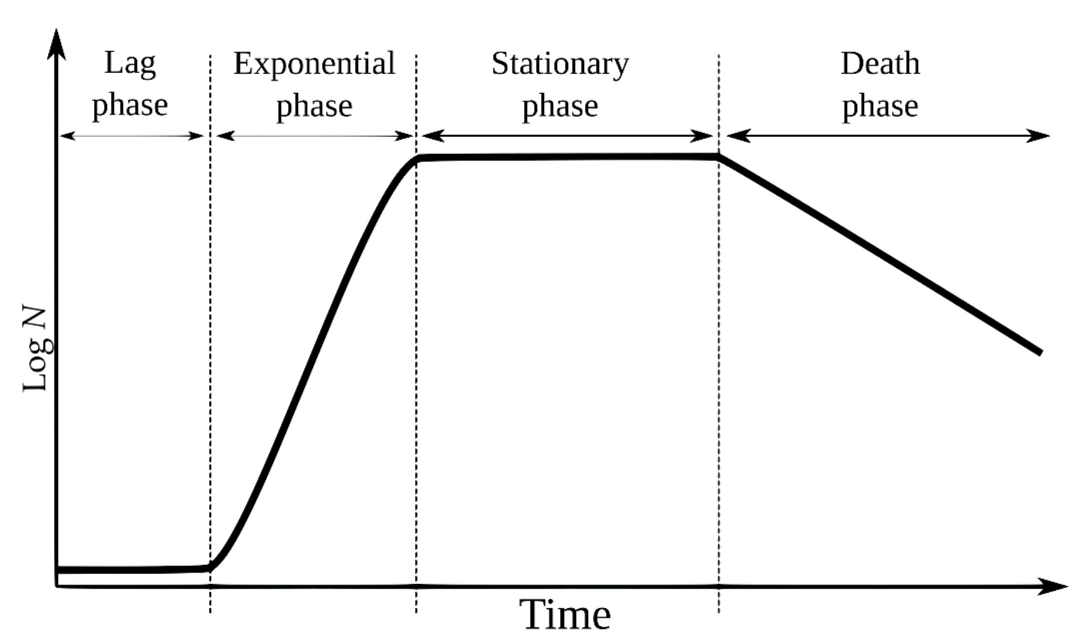
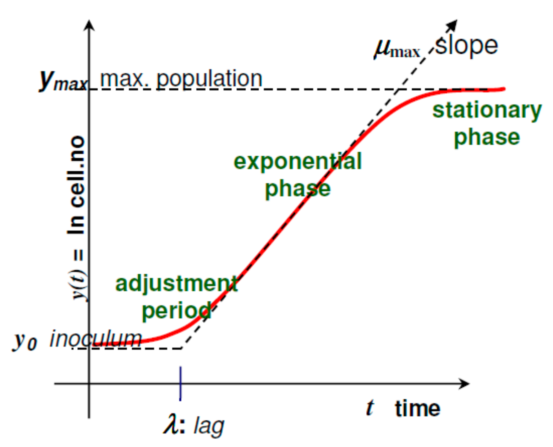
Lag or latency phase, characterized by the absence of microbial replication. The cells adapt to the environment, rich in nutrients, in order to initiate replication;

2.

Logarithmic or exponential phase, characterized by accelerated cell division;

3.

Stationary phase, characterized by the decline of the metabolic rate due to the depletion of nutrients in the environment;

4.

Death or logarithmic decline phase, characterized by the exponential decline of living cells and their growth.

Predictive models characterize microbial growth in each phase as a function of time (t), presenting different essential variables, such as the maximum specific growth rate (μ_max), the logarithmic increase in the microbial population (A) and the maximum microbial population reached (N_max). Estimating the length of lag phase (β) may be regarded as a good indicator of food shelf life, being influenced by factors such as the physiological state of bacteria or the conditions of the environment in which food is stored or displayed [6].

Whiting and Buchanan [7] suggested that predictive microbiology models could be categorized in three different forms, depending on the variables to consider:

• Primary models, in which variations of environmental factors are not considered. They only describe the concentration of microorganisms as a function of time;
• Secondary models, which consider variations in environmental factors, such as temperature (T), pH (potential of hydrogen) or water activity (a_w);
• Tertiary models: integrated models enhanced through computational modeling.

Among the existing predictive microbiology models, it is imperative to highlight the model proposed by Barany [8] and Barany and Roberts [9]. It is one of the most used primary models, due to its ability to adjust to data and its easily interpretable parameters. The model describes an approximate movement to a sigmoid curve, despite presenting an intermediate phase close to a straight line, unlike classic sigmoid curves.

One of the main limitations pointed out in primary models is the lack of biological foundations. Previously proposed algebraic models were deduced from insufficiently solid mechanistic considerations. There was a biological gap in these models, making it difficult to mechanically interpret the proposed parameters [10]. Based on this assumption, the model in question was developed in order to consider the biological mechanism of microorganisms’ growth. It introduced the concept of cellular physiological state (h₀), (defined as the effect of the history of cells, capable of influencing lag phase), providing the models hitherto proposed with greater biological suitability [10]. Figure 2 shows the adaptation of the four parameters adopted by Barany and Roberts [9] for the microbial growth curve.

The microbial growth parameters according to the model developed by Barany and Roberts [8], such as microbial population (y), logarithmic increase in microbial population (A) or length of lag phase (β), are obtained by adjusting the growth curve to the algebraic expressions given by Equations (1)–(3), respectively.

y(t) = y₀ + k·A(t) − ln (1 + [e^kA(t) − 1]/[e^ymax − y₀])

(1)

A(t) = t + (1/k) ln ([e^kt + q₀]/[1 + q₀])

(2)

β = (ln [1 + {1/q₀}])/k

(3)

Thus, the novelty of the approach in this study highlights the innovation and practical value of the decision support system that can contribute to the sustainable value of reducing food waste by providing information to retailers on the safety of their perishable evolution along time depending on storage conditions and suggesting a fair price depending on that quality. The decision-making tool may also encompass sustainable consumption from the consumers point of view.

3. Methods and Materials

3.1. Shelf Life Prediction Method

3.1.1. Intrinsic and Extrinsic Factors

A food item is a complex chemical matrix. Predicting whether or how quickly microorganisms will grow in a food product is a difficult task, given that most foods contain sufficient nutrients to promote microbial growth and each microorganism develops at a different rate and under different conditions. There are several factors that promote, restrict, or prevent bacterial growth in food products, and these can be grouped into two categories: intrinsic and extrinsic factors.

Intrinsic factors are the factors inherent to the food itself, which affect microbial growth, such as water activity, acidity, oxidation-reduction potential, chemical composition, or the biological structure of the food [11]. The intrinsic factors to consider in the development of the DSS are the water activity and acidity:

• Water activity (a_w): one of the intrinsic factors of products that are likely to promote microbiological growth, given that bacteria normally grow in environments where water is available. Water activity is defined as the ratio between the vapor pressure of water (p_v) in the food product and the saturated vapor pressure of water (p_sv) at the same temperature, as shown in Equation (4) [11]. Its value ranges from 0 (dry bone) and 1 (saturated water).

a_w = p_v/p_sv

(4)

a_w is directly influenced by the air relative humidity, φ. If the air in contact with a food product has lower φ, the water migrates to the air, increasing its φ and reducing the moisture content of the food, until equilibrium is reached. Conversely, if a food product with low a_w is stored in an environment with high φ, the a_w of this food will increase, promoting the multiplication of microorganisms [12]. In an isolated system, in which food products are in equilibrium with the relative humidity of the environment, the a_w of these foods may be defined by Equation (5).

a_w = φ/100

(5)

The precise a_w values of each food product are difficult to be defined due to the referred dependencies of the parameters.

Table 1. Water activity intervals for each horticultural product [13].

Product	Minimum aw Value	Average aw Value	Maximum aw Value
Lettuce	-	0.996	-
Onion	0.974	0.982	0.990
Carrot	0.983	0.988	0.993
Cabbage	0.990	0.991	0.992

shows the specific water activity values according to Chirife and Fontan [13] for each of the horticultural products covered in the DSS—lettuce, onion, carrot, and cabbage—in the form of minimum, average and maximum values.

• Potential of Hydrogen (pH): The level of acidity or basicity of a food product is measured by using a pH scale, defined as the inverse logarithm of the hydrogen ion activity in a solution given by Equation (6).

pH = log₁₀(1/a_H+)

(6)

The potential of hydrogen also plays an important part in bacterial growth. Each microorganism has an optimal pH value at which its multiplication is maximum. Both the increase and decrease in the acidity level in relation to the optimal value slows microbial growth [14]. A food’s own acidity also influences microbial growth. The reduction of pH of a food product contributes to the reduction in the capacity of bacterial development and vice versa [15].

Table 2. Potential of hydrogen intervals for each horticultural product.

Product	Minimum pH Value	Average pH Value
Lettuce	5.8	6.0
Onion	5.3	5.9
Carrot	4.9	6.4
Cabbage	5.2	6.9

specifies the typical pH values of the horticultural products under analysis according to [14,16]. These values are given in the form of an interval, due to the acidity variations that each product may present among itself, but also due to the existence of several species of each of these products, knowing that each species has its own characteristics—e.g., pH.

Regarding the extrinsic factors that affect bacterial growth, i.e., the factors inherent to the food´s external environment, the DSS only considers temperature:

• Temperature (T): The extrinsic temperature of a food item, i.e., the temperature of the environment in which it is stored, determines the ability of microbial organisms to multiply. As with pH, these organisms have an ideal temperature range that favors their multiplication. Both the increase and the decrease of the temperature in relation to its optimal value makes the microbial propagation slower [14]. Foodstuffs have their own specific optimal storage temperature, for which deterioration is minimal, including microbial growth, and the state of fullness is maximized. However, retailers must balance the extension of shelf life with the energy demand and the environmental impact of refrigeration systems and procedures, techniques and methods to improve both thermal performance and energy efficiency [17,18,19,20,21]. According to [22], the recommended storage temperature range for the vegetables analyzed is between 0 °C and 4 °C.

3.1.2. Bacterial Growth Prediction Method

The prediction of the remaining shelf life (SL) of a vegetable among the ones studied represents the crucial functionality of the developed DSS. It is carried out based on the growth model developed in [23], which, in turn, is founded on the predictive model proposed by [9]. ComBase (Combined Database for Predictive Microbiology) is an online predictive food microbiology platform with the main objective of describing and predicting how certain microorganisms survive and grow when conditioned by a series of factors inherent to the environment to which they are exposed, namely temperature, pH, or water activity [23]. The method adopted by the DSS to predict horticultural products´ shelf life is, in fact, a system that allows predicting the time that the infective dose of a certain growing bacterium takes to be reached, starting from a particular initial dose. Similar procedures were conducted by Gaspar et al. [24] that developed a simplified approach to predict food safety through the maximum specific bacterial growth rate as a function of extrinsic and intrinsic parameters.

Bacterial concentration values are given in terms of Colony Forming Units (CFU) per gram of product, with each bacterium having its own initial CFU and infective CFU doses.

Table 3. Initial and infective doses for each bacterium in study [23].

Bacteria	Initial Dose (CFU/g)	Infective Dose (CFU/g)
Aeromonas hydrophila	103	105
Bacillus cereus	101	105
Listeria monocytogenes	101	102
Salmonella	102	105
Shigella flexneri	100	102
Staphylococcus aureus	101	105

indicates initial and infective CFU doses for each one of the relevant bacteria according to [13,22], the growth analysis of which is available on [23]: Aeromonas hydrophila; Bacillus cereus; Listeria monocytogenes; Salmonella; Shigella flexneri; Staphylococcus aureus and, therefore, considered on the development of the DSS.

The time interval that is a DSS main output represents the period that includes the moment that the vegetable in study enters the retailer´s warehouse (the instant at which the respective bacterial doses will assume the value of the initial CFU established for each bacterium), to the moment in which the infective CFU value of each bacteria colony under study is reached.

In a particular horticultural product, different species of bacteria multiply. The shelf life of that product will be dictated by the bacteria colony that most rapidly reaches its infective dose. In other words, the bacterial growth (under the same storage conditions) of the different bacteria present in a same vegetable is studied. The time that each bacterium increasing colony needs to reach its infective dose are compared. The shortest of these times will, then, represent the shelf life of the studied horticultural product, given that, once the infective dose of any bacteria is reached, the product is no longer marketable as the food safety is compromised.

Table 4. Bacteria capable of growing in each horticultural products under study [23].

Bacteria	Lettuce	Onion	Carrot	Cabbage
Aeromonas hydrophila	X	X	X	X
Bacillus cereus	X	X	X	X
Listeria monocytogenes	X
Salmonella	X	X	X	X
Shigella flexneri		X	X
Staphylococcus aureus

outlines which bacteria mostly develop in each of the vegetables under study [14,25]. Thus, within the purpose of predicting the time inherent to bacterial growth for each of the horticultural products under analysis, the specific bacteria mentioned in Table 4, which growth in the respective vegetables had already been reported in the literature, will be studied.

The time until the infective dose of a bacterium replicating in a food item is reached will vary depending on the storage conditions of that product. Thus, the remaining shelf life of a product will essentially be dictated by its intrinsic and extrinsic factors: water activity, pH, and temperature. In addition to these factors, and as seen in Figure 3, two other inputs that influence bacterial growth are considered by the chosen predictive model [23], both of which are also mentioned above: the initial physiological state and the initial bacterial dose.

The initial physiological state was firstly introduced in the model proposed by Barany and Roberts [9]. It is the parameter associated to the first phase of bacterial growth, i.e., the lag or latency phase and, therefore, capable of influencing it. This parameter assumes a dimensionless number comprised between 0 and 1, which expresses the physical adaptation of cells to the environment. If its value is 0, growth will not occur (latency is infinite). If its value equals 1, growth will begin immediately (there is no latency phase). The length of lag phase depends not only on the surrounding environment (temperature, water activity, pH), but also on the history of the cells. Stresses (e.g., thermal or osmotic) may significantly increase latency times. Synthetically, the initial physiological state quantifies the effect of the cell’s history, which is reflected in the latency time of bacterial growth [23]. The lag time derives from initial physiological state of the cells through Equation (7).

lag = −log (Phys. State)/Max. rate

(7)

where “Phys. state” represents initial physiological state and “Max. Rate” the maximum slope of the growth curve. In the proposed method, to simulate the effect of the distribution chain on bacterial growth of vegetables, the initial physiological state input will assume, in all circumstances, its maximum value, set to 1. Thus, the lag phase will be disregarded in the bacterial growth model assumed by the DSS, being associated to the time that the horticultural products in analysis take to travel through their normal distribution chain. Thus, it is considered that bacterial growth begins at moment zero of the time interval considered by the DSS, which will represent the instant when the horticultural product in study enters the retailer’s warehouse, which is the last facility before being sold to the final consumer.

In addition to this assumption, the DSS database, built by extracting data from [23], will be constituted for each horticultural product in the study, by:

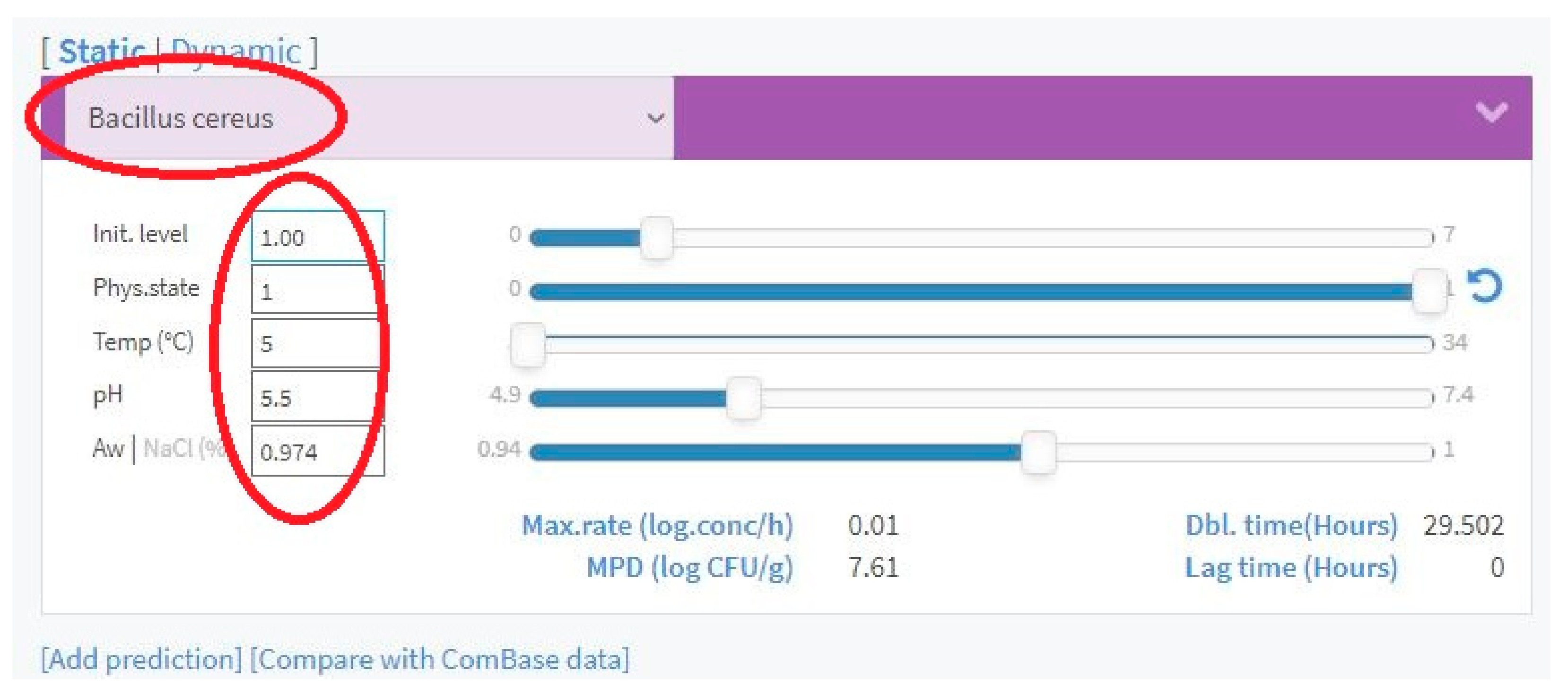
• Three different water activity scenarios, to simulate the effects of the relative humidity of the environment in the increasing bacterial doses. The adopted scenarios relate to the minimum, average, and maximum a_w values specific to each vegetable, as shown in Table 1. It is expected that the retailer, as the user of the DSS, would collect the a_w value that the horticultural product from a certain batch has when arriving at the final warehouse before being sold. Usually, it is impossible for the retailer to directly collect the product’s a_w value. Assuming that equilibrium conditions are reached within a short period [26], the air relative humidity must be collected or measured, making use of the relation between φ and a_w shown in Equation (5). Although not direct, this method for a_w value estimation is more intuitive, as it does not imply the need for any specific measuring instruments, nor the use of the complex measurement processes that come with it. Thus, it just becomes necessary to have an indicator or a meter that measures the relative humidity of the air in the storage environment. As horticultural products are highly perishable and, as such, stored under modified temperature (and, sometimes, air humidity) conditions due to a mechanical refrigeration system by vapor compression, it is common for these systems to have indicators for air temperature and relative humidity. These should be the values collected by the DSS users. Thus, this method becomes, more desirable to be adopted by the targeted users of the DSS. Since it is aimed at small retailers, it is not expected for them to have significant technical knowledge in the area.
• In a specific vegetable, for each a_w scenario (minimum, medium or maximum), the effects, on bacterial growth of combining various temperatures with the range of the intrinsic pH values of each horticultural product are studied. Thus, for every value of storage temperature, separately combined with the individual values of the complete pH range characteristic to the studied vegetable (as shown in Table 2), the number of hours necessary to reach the respective infective doses of the various bacteria in growth according to the prediction simulated in [23] are collected. For a given storage temperature value combined with a specific intrinsic pH value, the registered hourly intervals inherent to the different bacterial species under study are compared. The shortest value is defined as the remaining shelf life of that vegetable for the temperature and pH values and, ultimately, for a_w under study. This assumption is made that after a food item reaches the infective dose of a certain bacteria, its safety is compromised, even if the infective doses of the remaining growing bacteria still take a considerable time to be reached. The temperature range under study starts at the minimum value for which bacterial growth is already verified and goes up to the temperature value at which, for a particular bacterium under study, the registered time intervals, for the full range of inherent pH, are all less than 24 h. Thus, from vegetable to vegetable, the temperature range under study may differ at its beginning and/or at its end.

The adopted method entails some limitations, now succinctly exposed, even though most of it have been previously addressed throughout the method description:

• The adopted method performs a temporal prediction until bacterial contamination in a vegetable under analysis is reached, at which its safety is compromised. However, bacterial doses of food can be reduced through heat treatment processes applied when cooking the food item. In those cases, food security is once again represented, meaning that food may be consumed. This limitation becomes especially relevant when evaluating a batch of potatoes or cabbage that are horticultural products typically consumed in a cooked state. Therefore, it is considered that the time period calculated by the DSS taken as the remaining shelf life of a product represents a maximum commercialization period instead of a maximum consumption period;
• The simulation of the effects of the distribution chain on bacterial growth is given by disregarding lag phase. Thus, it is assumed that bacterial proliferation (the logarithmic phase) begins at the moment that the vegetable is stored at the retailer’s premises (the final stage before being marketed to its final consumer), defined as moment zero;
• Static analysis regarding the environment where vegetables are stored. In other words, there are no exchanges, in matters of extrinsic factors, with the surrounding environment. As a result, there is no values fluctuation in temperature and relative humidity values of the storage atmosphere. Therefore, these extrinsic aspects assume a constant value over time;

Since the method adopted to estimate shelf life is based on bacterial growth, the DSS and its respective purpose are limited, in terms of input and output, to the values of temperature and pH at which bacteria under the study grows. In other words, the DSS will only be able to predict the maximum commercialization period if the vegetable in the analysis is stored under conditions of temperature and pH included in the ranges in which bacteria, due to their specific growing requirements defined in

Table 5. Minimum, maximum and optimal parameters for bacterial growth.

Bacteria	Min. T (°C)	Opt. T (°C)	Max. T (°C)	Min. pH	Opt. pH	Max. pH	Min. aw	Opt. aw	Max. aw
Aeromonas hydrophila	2	27	37	4.6	6.7	7.5	0.974	0.998	1
Bacillus cereus	5	34	34	4.9	7.4	7.4	0.940	0.999	1
Listeria monocytogenes	1	40	40	4.4	6.9	7.5	0.934	0.994	1
Salmonella	7	37.5	40	3.9	6.4	7.4	0.973	0.997	1
Shigella flexneri	15	37	37	5.5	7.3	7.5	0.971	0.993	1
Staphylococcus aureus	7.5	30	30	4.4	6.5	7.5	0.907	0.990	1

[14,23], effectively multiply.

3.2. Dynamic Pricing Method

Dynamic pricing may be defined according to Liu et al. [27], as the attribution of different prices over time to a same product or to different products from the same category, considering the individual characteristics of each product or changes in its qualitative state. The task of setting dynamic prices on horticultural products, as perishable goods, based on multiple criteria proves to be arduous and inaccessible to all small retailers, as it requires them to detain information, in real time, about variables such as rate of deterioration, time of onset of deterioration, demand, price elasticity of demand, or unit storage cost, that are parameters considered in numerous pricing models. To simplify the pricing model to adopt, and considering the target market of the developed tool, variables such as those mentioned above are disregarded. Therefore, a pricing model is adopted in which the qualitative state, expressed in terms of remaining shelf life, is taken as the only criterion to be considered in the dynamic pricing of the marketed vegetables. Assuming the remaining shelf life of a horticultural product as the only criterion to consider in the calculation of dynamic selling prices, the price to be set each day will assume a linear decrease, as a function of the number of remaining shelf-life days, where there is a constant price decrease as the level of stocks decreases, as proposed by Zhao and Zheng [28]. Thus, the price to be set each day will steadily decrease as the end of the predicted commercialization period approaches. The proposed pricing model uses the following assumptions:

When the horticultural batch under study enters storage (t = 0), that is, at the time when the lag phase ends and bacterial proliferation begins, the selling price to be charged is at its maximum, without any discount applied. This condition is similar to the model proposed by Rabbani et al. [29], given that the horticultural batch under study is considered to be in the fullness of its microbiological characteristics. At this moment, the ideal and desirable sale scenarios are given, as selling products at this date implies maximum food safety for the consumer and maximum profit for the retailer;

At the end of the calculated commercialization period (t_f), i.e., at the moment immediately prior to reaching the infective dose of any of the bacteria growing in the studied vegetable, the selling price to be charged is as small as possible. Thus, the product is sold at cost price, in order to avoid losses for the retailer. This represents the sale scenario that must be avoid. In this case, it is assumed that food safety is at its lowest and the retailer’s profit is null;

The calculated end of sale date is never prior to the date that horticultural products under study enter the warehouse, and vice versa. In other words, it is considered that the studied produce batch goes through its normal distribution chain arriving at the retailer’s warehouse in proper microbial conditions representative of food safety.

From the assumptions stated above, the dynamic selling price for any given time t to be considered in the proposed DSS is given by Equation (8).

SP(t) = SP(0) − [SP(0) − SP(t_f)] [t/SL]

(8)

where:

• SP(0): initial selling price;
• SP(t_f): cost price;
• SL: linear decrease in price as a function of the studied vegetable estimated shelf life.

3.3. Decision Support System

Being necessary to adopt a platform to develop the proposed DSS, Microsoft Excel spreadsheet is selected, as it is a relatively intuitive and efficient tool for the DSS target market as well as the general population. The operation of the DSS will essentially rely on two important features provided by the aforementioned software: functions and macroinstructions. In addition to the need to correctly run Microsoft Excel software on a computer, enabling macro execution, the user is required to collect the various values necessary to serve as inputs to the DSS through a relative humidity measuring device; a thermometer or a storage temperature indicator; a pH measuring device, in order that the obtained outputs be as reliable as possible. Intrinsic factors can be provided by the producer while extrinsic factors can be provided by the air conditioning or refrigeration systems. The DSS consists of three functional interrelated areas: Database, Search Engine and User Interface:

• Database is constituted by the compilation of the data collected in [23], referring to the time frame until the infective dose of a certain bacterium is reached. The number of remaining hours until the infective dose of the considered bacteria is achieved is successively collected for each of the possible combinations set between a_w values, temperature and pH values under study for the vegetable under analysis;
• Search Engine includes all the mechanisms necessary to the processes of database searching, processing, and returning the respective treated information to the user, as a function of the inputs given, in terms of the intrinsic and extrinsic conditions of storage and dynamic pricing parameters. All processes developed in this functional area make use of search, information processing and calculation functions inherent to Microsoft Excel: “VLOOKUP”, “MIN”, “INDEX”, “MATCH” or “SEQUENCE”.
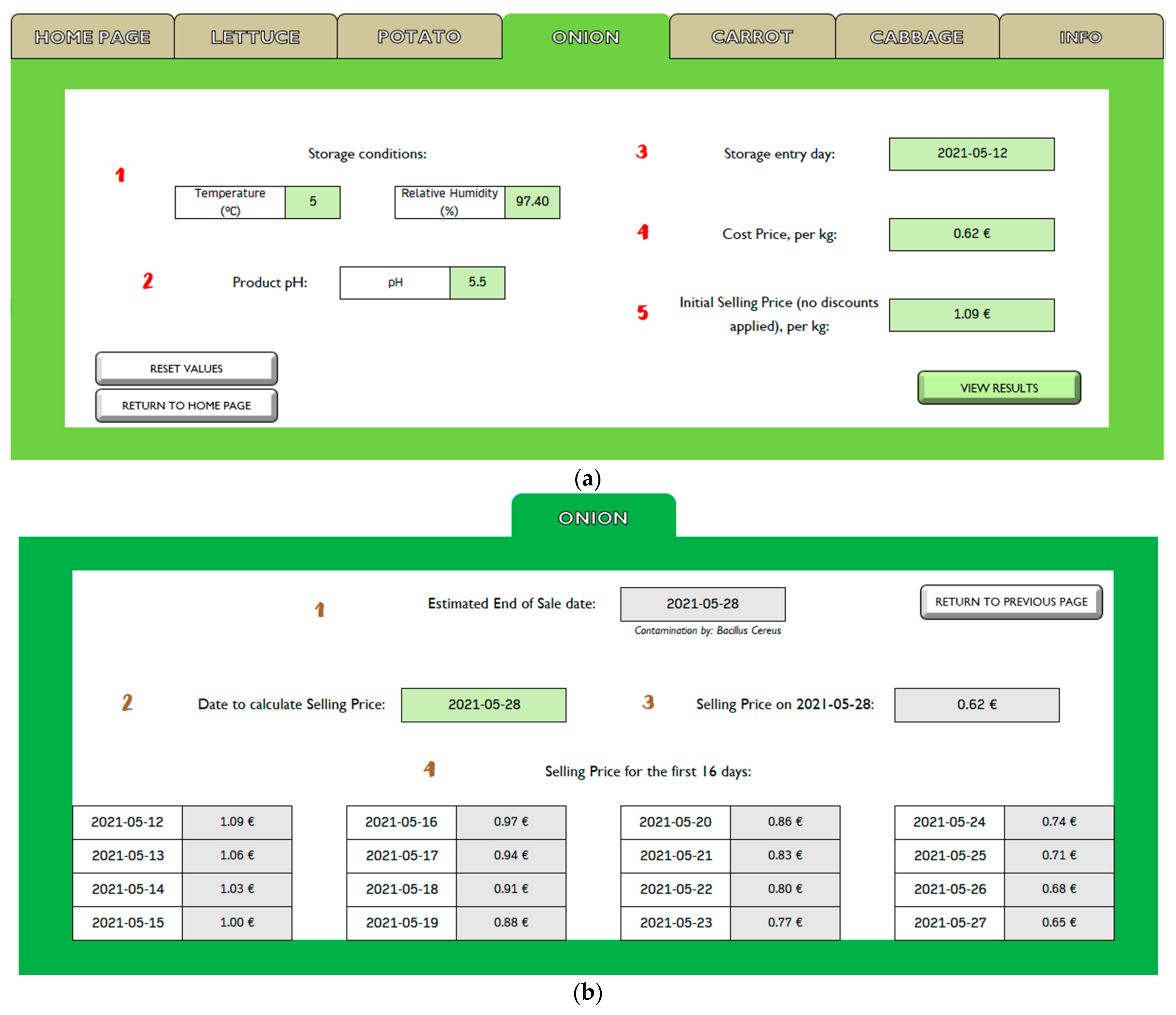
• User Interface (UI) serves as the DSS´s mean of interaction and communication with its user. This UI will be the only functional area of the DSS to which user will have access. The remaining components are inaccessible. Here, the necessary inputs in terms of shelf life prediction and price calculation are inserted, and the respective results are displayed.

Figure 4 exemplifies the interface shown to the user when analysing onion, as an example, with water activity, a_w = 0.974, which, by Equation (5) corresponds to an equilibrium relative humidity φ = 97.4%, a storage temperature, T = 5 °C and a pH = 5.5. Regarding the pricing parameters, the entry of the batch under analysis into the retailer’s warehouse (t = 0) is registered on 12 May 2021 is considered, so as an initial selling price (SP(0)) of €1.09 per kg and a cost price (SP(t_f)) of €0.62 per kg. As a result of the illustrated example, DSS estimates an end sale date on 2021-05-28 (date format: YYYY-MM-DD), 16 days after the studied onion batch was put into storage. This represents the date immediately prior to the moment when food safety is compromised through contamination by Bacillus cereus, so that, until the end of this date, the remaining onions on the batch must be sold at cost price (€0.62 per kg).

4. Case Studies

The obtained results, referring to the shelf lives of the studied vegetables, are individually sampled in this section, complemented by a proper analysis.

4.1. Case Study 1—Lettuce

In this case study in particular, a single water activity scenario (a_w = 0.996) was considered, as shown in Table 1, converted by Equation (5) into an equilibrium relative humidity scenario, φ = 99.6%. Regarding the bacteria considered for this vegetable, the growth of Aeromonas hydrophila, Bacillus cereus, Listeria monocytogenes and Salmonella was estimated. The analysis of this horticultural product starts at T = 1 °C, temperature in which Listeria Monocytogenes starts to replicate, and ends at T = 10 °C, temperature at which, for every pH value, food safety threshold is reached in t ≤ 24 h. In other words: at T = 10 °C, regardless the pH value in analysis, the remaining marketing period will always be less than 24 h. At the end of this period, the food safety threshold is reached through contamination by, in this case, Listeria monocytogenes. For this reason, any higher temperature values are disregarded by the DSS, given that the obtained commercialization period will always be inferior to 24 h, and, therefore, irrelevant for pricing purposes. In matters of pH, values between 5.8 ≤ pH ≤ 6.0 were considered, according to Table 2. The sampling of the results obtained in the study of lettuce, concerning its remaining shelf life, is shown in

Table 6. Sampling of results of DSS—Remaining shelf life of lettuce.

T (°C)	pH	aw	Remaining Shelf Life (t, in Hours)	Contamination by
1	5.8	0.996	155.20	Listeria monocytogenes
	5.9	0.996	146.00	Listeria monocytogenes
4	5.8	0.996	79.60	Listeria monocytogenes
	5.9	0.996	73.60	Aeromonas hydrophila
10	5.9	0.996	22.10	Aeromonas hydrophila
	6.0	0.996	20.50	Aeromonas hydrophila

. The presented results immediately allow the observance of the influence of temperature on shelf life of this vegetable. Among the studied combinations, in the most unfavourable scenario for bacterial growth, minimum temperature and pH values (T = 1 °C; pH = 5.8) and, as such, more favourable for the conservation of foodstuffs, a shelf life of t = 155.2 h after the horticultural enters storage is predicted at the threshold of contamination by Listeria monocytogenes. This is the only bacterium capable of replicating under such conditions. On the other hand, when the selected temperature and pH values are at their maximum for the range under study (T = 10 °C; pH = 6.0) and, therefore providing the most favourable scenario for bacterial replication, shelf life is dictated when contamination by Aeromonas hydrophila is reached, after t = 20.5 h of storage. Under these storage conditions, and as the most favourable scenario for bacterial growth, the proliferation of every bacteria under study is registered. In the stated sample, there were no observed cases of contamination by Bacillus cereus or Salmonella. In this particular case study, it was not possible to determine the effect of relative humidity on the lifetime of the horticultural product, due to the lack of a comparison term, since only a water activity value found in the literature was considered.

4.2. Case Study 2—Onion

This case study considers a_w = 0.974, 0.982 and 0.990, resulting in relative humidity scenarios of φ = 97.4%, 98.2% and 99%, respectively. The growth of Aeromonas hydrophila, Bacillus cereus, Salmonella and Shigella flexneri was considered. The analysis of this vegetable starts at T = 2 °C, the temperature at which Aeromonas hydrophila starts replicating, ending at T = 18 °C, for the reasons already mentioned. This is the temperature value at which the relative humidity scenario is more conducive to microbial growth, and the food safety threshold is reached in less than 24 h, for the full range of combined pH values, by reaching the infective dose of Hydrophila aeromonas. Regarding the acidity levels in the study, pH values inherent to the onion itself were considered, comprised between 5.3 ≤ pH ≤ 5.9. The sampling of the results of remaining shelf life for onion is shown in

Table 7. Sampling of results of DSS—Remaining shelf life of onion.

T (°C)	pH	aw	Remaining Shelf Life (t, in Hours)	Contamination by
2	5.3	0.974	1580.4	Aeromonas hydrophila
		0.982	728.8	Aeromonas hydrophila
		0.990	354.6	Aeromonas hydrophila
	5.4	0.974	1359.0	Aeromonas hydrophila
		0.982	628.8	Aeromonas hydrophila
		0.990	307.8	Aeromonas hydrophila
10	5.5	0.974	179.7	Bacillus cereus
		0.982	102.4	Aeromonas hydrophila
		0.990	50.6	Aeromonas hydrophila
	5.6	0.974	173.4	Bacillus cereus
		0.982	90.2	Aeromonas hydrophila
		0.990	44.8	Aeromonas hydrophila
18	5.7	0.974	35.8	Salmonella
		0.982	23.9	Aeromonas hydrophila
		0.990	12.0	Aeromonas hydrophila
	5.8	0.974	34.9	Salmonella
		0.982	21.7	Aeromonas hydrophila
		0.990	11.0	Aeromonas hydrophila

.

When, at the lowest analysed temperature (T = 2 °C), equal pH values in different water activities are compared, a large disparity caused by the different relative humidity scenarios is verified. For example, when T = 2 °C and pH = 5.4, for a_w = 0.974, 0.982 and 0.990, the remaining shelf lives are, respectively, t = 1580.4, 728.8 and 354.6 h. Alternating between minimum and maximum relative humidity scenarios implies a decrease of Δt = 1225.8 h in the estimated remaining shelf life. However, this differential decreases significantly as storage temperatures increase. When T = 10 °C and pH = 5.6, shelf life is limited to t = 173.4, 90.2 and 44.8 h for a_w = 0.974, 0.982 and 0.990, respectively, a difference of Δt = 128.6 h between the most extreme scenarios. At the highest temperature among those observed (T = 18 °C), for the same pH value, contamination by different bacteria is registered, depending on the water activity value in question. At a pH = 5.8 when a_w = 0.974, there is contamination by Salmonella. If, in turn, a_w = 0.982 or 0.990, contamination is set by reaching the infective dose of Aeromonas hydrophila.

At the most unfavourable scenario for bacterial growth, that is, the minimum water activity, temperature, and pH values (a_w = 0.974; T = 2 °C; pH = 5.3), the shelf life is reached t = 1580.4 h after the horticultural batch entrance into storage, at the threshold of contamination by Aeromonas hydrophila, as it is the only bacterium capable of replicating under the selected conditions. On the other hand, when the selected water activity, temperature and pH values are maximum for the range under study (a_w = 0.990; T = 18 °C; pH = 5.9) and, therefore, provide the most favourable scenario for bacterial replication, shelf life is dictated when the contamination threshold is reached, and also by Aeromonas hydrophila, after t = 11 h of storage. In this sample, no cases of contamination by Shigella flexneri were predicted.

4.3. Case Study 3—Carrot

It was considered for the study of carrot that a_w = 0.983, 0.988 and 0.993, resulting in equilibrium relative humidity scenarios of 98.3%, 98.8% and 99.3%, respectively. The growth of Aeromonas hydrophila, Bacillus cereus, Salmonella and Shigella flexneri were studied for this vegetable. The analysis starts at T = 2 °C, at which the onset of proliferation of Aeromonas hydrophila is verified. For the reasons already mentioned, the study interval is delimited by Aeromonas hydrophila, at T = 19 °C. The study range includes the pH values inherent to the carrot itself, comprised between 4.9 ≤ pH ≤ 6.4. The sampling of the results obtained in the study of carrot concerning the remaining shelf life is shown in

Table 8. Sampling of results of DSS—Remaining shelf life of carrot.

T (°C)	pH	aw	Remaining Shelf Life (t, in Hours)	Contamination by
2	4.9	0.983	1321.6	Aeromonas hydrophila
		0.988	829.0	Aeromonas hydrophila
		0.993	541.2	Aeromonas hydrophila
	5.0	0.983	1096.2	Aeromonas hydrophila
		0.988	689.0	Aeromonas hydrophila
		0.993	451.8	Aeromonas hydrophila
10	4.9	0.983	152.4	Bacillus cereus
		0.988	126.4	Bacillus cereus
		0.993	101.4	Aeromonas hydrophila
	5.0	0.983	148.0	Bacillus cereus
		0.988	123.0	Bacillus cereus
		0.993	84.6	Aeromonas hydrophila
19	6.3	0.983	13.6	Aeromonas hydrophila
		0.988	9.0	Aeromonas hydrophila
		0.993	6.2	Aeromonas hydrophila
	6.4	0.983	13.1	Aeromonas hydrophila
		0.988	8.6	Aeromonas hydrophila
		0.993	6.0	Aeromonas hydrophila

. As seen in the previous case study, at the lowest temperature under analysis (T = 2 °C), when comparing different water activities at the same pH value, a relevant differential is determined, caused by the different relative humidity scenarios proposed. When T = 2 °C and pH = 5.0, for a_w values = 0.983, 0.988 and 0.993, t = 1096.2, 689.0 and 451.8 h of remaining shelf life is estimated, respectively. Thus, alternating between minimum and maximum relative humidity scenarios implies a decrease of Δt = 644.4 h in the remaining shelf life. However, it is seen that this differential decreases significantly as storage temperatures increase.

When comparing different pH values under the same conditions of temperature and water activity, there is a rather considerable difference at low temperatures, which gradually becomes residual at higher temperatures. At T = 2 °C and a_w = 0.988, shelf life assumes t = 829 h when pH = 4.9 and t = 689 h when pH = 5.0, a difference of Δt = 140 h. When storage temperature assumes a value of T = 10 °C and the water activity value remains unchanged (a_w = 0.988), shelf life is t = 126.4 h for a pH = 4.9 and t = 123 h for a pH = 5.0, that is, a difference of Δt = 3.4 h. At the most unfavourable scenario for bacterial growth, minimum water activity, temperature, and pH values (a_w = 0.983; T = 2 °C; pH = 4.9), the shelf life t = 1321.6 h after the horticultural batch enters storage is established at the threshold of contamination by Aeromonas hydrophila (the only bacterium capable of replicating under the selected conditions). When the water activity, temperature and pH values are maximum for the range under study (a_w = 0.993; T = 19 °C; pH = 6.4), providing the most favourable conditions for bacterial replication, shelf life is dictated when the contamination threshold is reached, also by Aeromonas hydrophila, after t = 6 h of storage. The analysed sample is strongly influenced by the contamination by Aeromonas hydrophila. In the same sample, no cases of contamination by Salmonella or Shigella flexneri were observed.

4.4. Case Study 4—Cabbage

For the last case study, a_w = 0.990, 0.991 and 0.992 were considered, originating, in turn, with relative humidity scenarios of φ = 99%, 99.1% and 99.2%, respectively. For the study of this product, the bacterial growth of Aeromonas hydrophila, Bacillus cereus and Salmonella were considered. The analysis of cabbage begins at a storage temperature of T = 2 °C, at which the onset of proliferation of Aeromonas hydrophila is verified. The study interval is also delimited by Aeromonas hydrophila, at T = 17 °C. In terms of acidity, the study range includes pH values between 5.2 ≤ pH ≤ 6.9. The sampling of the results obtained in the study of cabbage concerning remaining shelf life is shown in

Table 9. Sampling of results of DSS—Remaining shelf life of cabbage.

T (°C)	pH	aw	Remaining Shelf Life (t, in Hours)	Contamination by
2	5.2	0.990	413.4	Aeromonas hydrophila
		0.991	380.4	Aeromonas hydrophila
		0.992	350.4	Aeromonas hydrophila
	5.3	0.990	354.6	Aeromonas hydrophila
		0.991	327.6	Aeromonas hydrophila
		0.992	301.8	Aeromonas hydrophila
9	6.0	0.990	36.6	Aeromonas hydrophila
		0.991	34.0	Aeromonas hydrophila
		0.992	31.6	Aeromonas hydrophila
	6.1	0.990	34.2	Aeromonas hydrophila
		0.991	31.7	Aeromonas hydrophila
		0.992	29.4	Aeromonas hydrophila
17	6.8	0.990	8.7	Aeromonas hydrophila
		0.991	8.1	Aeromonas hydrophila
		0.992	7.6	Aeromonas hydrophila
	6.9	0.990	8.8	Aeromonas hydrophila
		0.991	8.2	Aeromonas hydrophila
		0.992	7.7	Aeromonas hydrophila

.

The sample analysed in cabbage study is strongly marked by contamination by Aeromonas hydrophila, given that, for the combinations shown, there is no contamination by any of the remaining bacteria considered.

At the most unfavourable scenario for bacterial growth: water activity, storage temperature and pH at minimum values (a_w = 0.990; T = 2 °C; pH = 5.2), the shelf life is limited to t = 413.4 h after the entrance of the batch of the studied horticultural product into storage is established at the threshold of contamination by the only bacteria capable of replicate under those conditions, Aeromonas hydrophila. At the inverse end of the study range, when the selected values for water activity, temperature and pH are maximum, given the study range (a_w = 0.992; T = 17 °C; pH = 6.9), shelf life is dictated when food safety threshold is reached, after t = 7.7 h of storage. At an intermediate storage scenario (a_w = 0.991; T = 9 °C; pH = 6), a remaining shelf life of t = 34 h is estimated.

5. Discussion

The subsequent analysis is based on the comparison of the values predicted by the DSS, in matters of shelf life, with the values collected in literature [30,31,32]. Comparison between optimal storage conditions ascertained in literature (0 to 4 °C) and the conditions most favourable for food preservation capable of being analysed by the DSS (minimum a_w, T and pH values) are listed in

Table 10. Comparison between the shelf time values obtained by the DSS and the values collected in literature.

	Literature [30,31,32]				DSS
	T (°C)	φ (%)	pH	SL (Days)	T (°C)	φ (%)	pH	SL (Days)
Lettuce	0	95–100	-	7–21	1	99.6	5.8	6
Onion	0	65–75	-	14–91	2	97.4	5.3	66
Carrot	0	95–100	-	31–152	2	98.3	4.9	55
Cabbage	0	95–100	-	21–42	2	99.0	5.2	17

. Given that the times collected in the literature do not specify pH values, it is assumed they already consider variations resulting from the different acidity values specific to each horticultural product under study.

It must be noticed that, in a general way, the values obtained by the DSS are somewhat lower than the literature. According to [30,31], when storing lettuce at a temperature of T = 0 °C, in an atmosphere with relative humidity set between 95% ≤ φ ≤ 100%, a remaining shelf life of 7 ≤ t ≤ 21 days is indicated. The developed DSS, on the other hand, determines a remaining shelf life of t = 6 days, when the storage temperature is fixed at T = 1 °C, pH = 5.8 and relative humidity φ = 99.6%. This value turns out to be somewhat lower than the range collected in the literature.

DSS determines for the case study of onion, SL values that meet the ones collected bibliographically. When storage occurs at T = 2 °C, φ = 97.4% and the vegetable’s pH = 5.3, the developed tool estimates a remaining shelf life of t = 66 days. In [31,32], a SL between 14 ≤ t ≤ 91 days is indicated, when storage occurs at T = 0 °C and 65% ≤ φ ≤ 75%. However, the large divergence between the values for storage relative humidity pointed in both cases should be noted.

The carrot case study also points to very consistent values in both cases, when storage conditions are the most favourable to the preservation of this product. The developed DSS estimates a SL value of t = 66 days, while a value in the range of 31 ≤ t ≤ 152 is collected in [30,31].

When it comes to the last studied product, cabbage, and similarly to what was observed in the study of lettuce, DSS canvasses SL values that are slightly lower compared to those collected in the literature. When stored at a relative humidity of φ = 99%, temperature of T = 2 °C and for a pH = 5.2, the DSS predicts t = 17 days. In [30,31], a remaining SL for cabbage is found to be comprised between 21 ≤ t ≤ 42 days, when stored at T = 0 °C and 95% ≤ φ ≤ 100%.

The practical implications of this study are related to a new approach to predict the shelf life of fresh horticultural products that have direct impact on the logistics sector by easing the decision-making around when and where to sell products. This condition is directly related to food waste and the profit of these companies. The practical implications for the small retailers and grocers are directly related to the availability of a simple and expedited decision support system that can be used in the everyday life that predicts not only the available shelf life of the stored and displayed horticultural products but also their price depending on the predicted safety. Academically, this new approach provides future research opportunities. This approach can be followed to include other horticultural products or even of food products beside horticultural ones, and developing experimental tests related to the comparison of the predicted and real values of organoleptic characteristics.

6. Conclusions

A decision support system (DSS) is proposed to simultaneously help reduce food waste for traditional food retailers while allowing for the selling of fresh horticultural products and promoting food safety and quality. This computational DSS allows for the predicting of the remaining shelf life of fresh horticultural products, namely lettuce, onion, carrot, and cabbage, based on its microbial growth status, governed by extrinsic (temperature and water activity) and intrinsic parameters (pH). The online predictive food microbiology tool Combined Database for Predictive Microbiology (Combase) was used to predict the time to reach the infectious doses of bacteria considered in the study. Additionally, the DSS encompasses the dynamic price of the produce that should be set each day, depending on the predicted end of the marketing period.

The shelf life determined by the DSS for optimal storage conditions is, in general, conservative, ensuring food safety. The prediction of shelf life through multiple criteria is reflected in the inaccuracy of times reflected in the literature, since these intervals present large amplitudes. Furthermore, when considering the remaining shelf life of a food item, priority should always be given to the microbiological criterion over others, given that a product may present satisfactory sensory indices and, at a same time, carrying microbial doses that go beyond safety threshold, thus rendering itself harmful to the consumer. It is considered, thus, that the conservative prediction provided by the DSS is aligned with the growing demand in matters of safety and quality required by all parts of the food chain, from the producer to the consumer, including wholesalers and retailers, as well as regulatory and governmental entities.

It should also be noted that small deviations between the values collected in the literature and the values estimated by the DSS were observed. In the case study of the onion, despite the obtained results being strongly aligned with the literature, other humidity scenarios closer to the optimal storage conditions should be investigated, as a humidity content set between 65% and 75% results in a drier storage environment than the one proposed by the current model.

Regarding the analysis of bacterial growth in each of the studied vegetables, in the sampled cases analysed, most shelf lives are set by contaminations of Aeromonas hydrophila, so it is considered that this bacterial colony most influences the DSS results. The versatility in the growth requirements inherent to this bacterial colony may justify this fact, given that it has a large pH and, especially, survives in a wide range of temperatures.

For the adoption of the DSS and its effective usage by its target market, it is considered that it still needs to undergo some. First, the studied water activity scenarios should be extended beyond the currently proposed minimum, average, and maximum values, undergoing adaptations whenever necessary. This refinement becomes particularly important in cases in which the difference between the water activity scenarios proves to be considerable in terms of remaining shelf life, as seen in the onion and carrot case studies at reduced storage temperatures. The effects of vegetables’ regular distribution chain on bacterial growth should be quantified more effectively than by simply disregarding the lag phase, since this parameter may affect, both positively and negatively, the estimated remaining shelf life of a food product. Finally, fluctuations of extrinsic factors in the storage environment should be considered. The proposed model assumes that the temperature and relative humidity of the storage environment remains constant over time, from the moment that the horticultural batch under study enters storage until the moment it is marketed. This assumption does not translate in practice, even though these fluctuations may be residual.

The proposed DSS contributes to sustainable development by promoting information to retailers and encouraging sustainable consumption based on perishable horticultural safety and quality across time and fair pricing depending on that quality.

References

1. FAO. World Food and Agriculture—Statistical Yearbook 2020; FAO-Food & Agriculture Organization of the United Nation: Rome, Italy, 2020. [Google Scholar]
2. Ross, T.; McMeekin, T.A. Predictive microbiology. Int. J. Food Microbiol. 1994, 23, 241–264. [Google Scholar] [CrossRef]
3. McMeekin, T.A.; Bowman, J.; McQuestin, O.; Mellefont, L.; Ross, T.; Tamplin, M. The future of predictive microbiology: Strategic research, innovative applications and great expectations. Int. J. Food Microbiol. 2008, 128, 2–9. [Google Scholar] [CrossRef] [PubMed]
4. Esty, J.R.; Meyer, K.F. The heat resistance of the spores of B. botulinus and allied anaerobes. XI. J. Infect. Dis. 1922, 31, 650–663. [Google Scholar] [CrossRef]
5. Štumpf, S.; Hostnik, G.; Primožič, M.; Leitgeb, M.; Bren, U. Generation times of E. coli prolong with increasing tannin concentration while the lag phase extends exponentially. Plants 2020, 9, 1680. [Google Scholar] [CrossRef] [PubMed]
6. Swinnen, I.A.; Bernaerts, K.; Dens, E.J.; Geeraerd, A.H.; Van Impe, J.F. Predictive modelling of the microbial lag phase: A review. Int. J. Food Microbiol. 2004, 94, 137–159. [Google Scholar] [CrossRef] [PubMed]
7. Whiting, R.C.; Buchanan, R.L. A classification of models for predictive microbiology. Food Microbiol. 1993, 10, 175–177. [Google Scholar]
8. Baranyi, J. Modelling and Parameter Estimation of Bacterial Growth with Distributed Lag Time. Ph.D. Thesis, University of Szeged, Szeged, Hungary, 2010. [Google Scholar]
9. Barany, J.; Roberts, T.A. A dynamic approach to predicting bacterial growth in food. Int. J. Food Microbiol. 1994, 23, 277–294. [Google Scholar] [CrossRef]
10. Subramaniam, P.; Wareing, P. The Stability and Shelf Life of Food, 2nd ed.; Woodhead Publishing: Cambridge, UK, 2016. [Google Scholar]
11. Gaspar, P.D.; Domingues, C.; Gonçalves, L.C.; Andrade, L.P. Avaliação da qualidade e segurança alimentar pela previsão do crescimento microbiano em diferentes condições de conservação. In Proceedings of the V Congreso Ibérico y III Congreso Iberoamericano de Ciencias y Técnicas del Frío, Castellón, Spain, 23–25 September 2009; Sociedad Española de Ciencias y Técnicas del Frío: Murcia, Spain, 2009. [Google Scholar]
12. Rahman, M. Handbook of Food Preservation, 2nd ed.; CRC Press: Boca Raton, FL, USA, 2007. [Google Scholar]
13. Chirife, J.; Fontan, C.F. Water activity of fresh foods. J. Food Sci. 1982, 47, 661–663. [Google Scholar] [CrossRef]
14. FDA. Bad Bug Book, Foodborne Pathogenic Microorganisms and Natural Toxins, 2nd ed.; U.S. Food and Drug Administration: Silver Spring, MD, USA, 2012.
15. Lund, B.; Baird-Parker, A.C.; Gould, G.W. Microbiological Safety and Quality of Food, 1st ed.; Springer: New York, NY, USA, 2000. [Google Scholar]
16. Bridges, M.A.; Mattice, M.R. Over two thousand estimations of the pH of representative foods. Dig. Dis. Sci. 1939, 6, 440–449. [Google Scholar] [CrossRef]
17. Gaspar, P.D.; Silva, P.D.; Nunes, J.; Andrade, L.P. Characterization of the specific electrical energy consumption of agrifood industries in the central region of Portugal. In Applied Mechanics and Materials; Trans Tech Publications Ltd.: Freienbach, Switzerland, 2014; Volume 590, pp. 878–882. [Google Scholar]
18. Nunes, J.; Silva, P.D.; Andrade, L.P.; Gaspar, P.D. Characterization of the specific energy consumption of electricity in the Portuguese sausage industry. WIT Trans. Ecol. Environ. 2014, 186, 763–774. [Google Scholar]
19. Silva, P.D.; Gaspar, P.D.; Nunes, J.; Andrade, L.P. Specific electrical energy consumption and CO2 emissions assessment of agrifood industries in the central region of Portugal. In Applied Mechanics and Materials; Trans Tech Publications Ltd.: Freienbach, Switzerland, 2014; Volume 675–677, pp. 1880–1886. [Google Scholar]
20. Gaspar, J.P.; Gaspar, P.D.; Silva, P.D.; Simões, M.P.; Santo, C.E. Energy Life-Cycle Assessment of Fruit Products—Case Study of Beira Interior’s Peach (Portugal). Sustainability 2018, 10, 3530. [Google Scholar] [CrossRef] [Green Version]
21. Gaspar, P.D.; Gonçalves, L.C.C.; Pitarma, R.A. CFD parametric studies for global performance improvement of open refrigerated display cabinets. Model. Simul. Eng. 2012, 2012, 54. [Google Scholar] [CrossRef] [Green Version]
22. Mercantila, F. Guide to Food Transport: Fruit and Vegetables; Mercantila Publishers: Copenhagen, Denmark, 1989. [Google Scholar]
23. ComBase—Combined Database for Predictive Microbiology. Available online: https://www.combase.cc (accessed on 14 March 2020).
24. Gaspar, P.D.; Alves, J.; Pinto, P. Simplified approach to predict food safety through the maximum specific bacterial growth rate as function of extrinsic and intrinsic parameters. ChemEngineering 2021, 5, 22. [Google Scholar] [CrossRef]
25. Baptista, P.; Venâncio, A. Os Perigos para a Segurança Alimentar no Processamento de Alimentos; Forvisão-Consultoria em Formação Integrada: Guimarães, Portugal, 2003. [Google Scholar]
26. Imre, L. The Measurement of Equilibrium Relative Humidity, Part II. Period. Polytech.-Bp. Univ. Technol. Econ. 1964, 8, 227–242. [Google Scholar]
27. Liu, X.; Tang, O.; Huang, P. Dynamic pricing and ordering decision for the perishable food of the supermarket using RFID technology. Asia Pac. J. Mark. Logist. 2008, 20, 7–22. [Google Scholar] [CrossRef]
28. Zhao, W.; Zheng, Y.S. Optimal dynamic pricing for perishable assets with nonhomogeneous demand. Manag. Sci. 2000, 46, 375–388. [Google Scholar] [CrossRef]
29. Rabbani, M.; Zia, N.P.; Rafiei, H. Joint optimal dynamic pricing and replenishment policies for items with simultaneous quality and physical quantity deterioration. Appl. Math. Comput. 2016, 287, 149–160. [Google Scholar] [CrossRef]
30. FAO. Prevention of Post-Harvest Food Losses: Fruits, Vegetables and Root Crops—A Training Manual; Food and Agriculture Organization of the United Nations: Rome, Italy, 1989. [Google Scholar]
31. Engineering ToolBox—Fruits and Vegetables Optimal Storage Conditions. Available online: https://www.engineeringtoolbox.com/fruits-vegetables-storage-conditions-d_710.html (accessed on 15 March 2020).
32. USDA—Commercial Item Description: Onions, Bulb, Ready-to-Use. Available online: https://www.ams.usda.gov/sites/default/files/media/A-A-20193D_Onions_Bulb_RTU.pdf (accessed on 22 April 2021).
Figure 1. Generic microbial growth curve [5].
Asi 04 00080 g001
Figure 2. Microbial growth curve with description of the four parameters considered in the model proposed by [9]. (Reprinted from ref. [8]).
Asi 04 00080 g002
Figure 3. Inputs required for predicting bacterial growth in Combase [23].
Asi 04 00080 g003
Figure 4. DSS user interface exemplified on onion: (a) Entering data regarding storage conditions and pricing; (b) Visualization of the obtained results.
Asi 04 00080 g004