Abstract
Aiming at the problem of the large tracking error of the desired curve for the automatic train operation (ATO) control strategy, an ATO control algorithm based on RBF neural network adaptive terminal sliding mode fault-tolerant control (ATSM-FTC-RBFNN) is proposed to realize the accurate tracking control of train operation curve. On the one hand, considering the state delay of trains in operation, a nonlinear dynamic model is established based on the mechanism of motion mechanics. Then, the terminal sliding mode control principle is used to design the ATO control algorithm, and the adaptive mechanism is introduced to enhance the adaptability of the system. On the other hand, RBFNN is used to adaptively approximate and compensate the additional resistance disturbance to the model so that ATO control with larger disturbance can be realized with smaller switching gain, and the tracking performance and anti-interference ability of the system can be enhanced. Finally, considering the actuator failure and the control input limitation, the fault-tolerant mechanism is introduced to further enhance the fault-tolerant performance of the system. The simulation results show that the control can compensate and process the nonlinear effects of control input saturation, delay, and actuator faults synchronously under the condition of uncertain parameters, external disturbances of the system model and can achieve a small error tracking the desired curve.
1. Introduction
Urban rail transit’s ATO (Automatic Train Operation system) is a direct unit responsible for the train’s safe operation and control, and its advanced control algorithm is the key to ensure the train’s efficiency, punctuality, control accuracy, comfort, and energy conservation [1]. In the case of the changeable operation environment and the system state changing, ATO control algorithm with high control accuracy, fast response speed, and less braking times is the core to ensure the tracking operation control of multiple trains under moving block [2].
In the process of the development of ATO, there are many different train operation control algorithms, and some achievements have been made, such as PID control [3], fuzzy control [4], adaptive control [5], iterative learning control [6], genetic algorithm control [7], predictive control [8], etc. However, the response speed of PID control is slow, which cannot meet the real-time requirements of train control. The adjustment of fuzzy control parameters and control rules is time-consuming and labor-consuming and needs experienced engineers to design, so it is not easy to implement in the project. Additionally, in the design process of the controller, the quasi parameters of the model need to be known in advance, but the parameters of the train operation model change with the changes of the train load, performance, and operating environment. The authors of [9] introduced an adaptive control to better overcome the control inaccuracy caused by the uncertainty of model parameters. However, there are certain limitations in the way of dealing with the additional resistance of the route. When facing the line slope change point, the switching of control input is too frequent, which affects the service life of the train braking system equipment. In order to overcome the problem of frequent switching of control input caused by adaptive control, [10] introduced an auxiliary system to control variable slope points smoothly. Although the adaptive control algorithm can make the system stable, when the route disturbance is large, the train operation state cannot converge quickly. The authors of [11] applied iterative learning control to realized train precise control. After repeated learning many times, the train can finally overcome the interference of the operation environment, but the real-time performance of continuous iteration is poor. The authors of [12] applied parameter estimation to realized on-line identification of train model parameters, and a fuzzy predictive control algorithm is designed, which can better deal with the uncertainty and external disturbance of model parameters. However, the problem of control accuracy degradation due to the limit value, delay, and the fault of many links such as an actuator, speed sensor, and interface equipment are not considered. In [13], a robust adaptive and fault-tolerant control scheme for high-speed trains is established by constructing a Lyapunov function with virtual parameter estimation error to ensure the safe and reliable operation of trains in normal conditions or in case of traction or braking failure. However, only the faults of the traction or braking mechanism are considered in the literature, and the control problems caused by input saturation and speed delay are not considered. In [14], an iterative learning control algorithm considering speed constraints is proposed to realize train operating curve tracking under the condition of variable parameters, but it does not involve the safe train operating control under input saturation and actuator traction or braking failure. In [15], a train adaptive iterative learning control method with speed delay and input saturation is designed, and the Lyapunov–Krasovskii function method is used to solve the problem of speed delay. In [16], an adaptive fault-tolerant ATO control method considering input saturation and speed delay is proposed, and the convergence of speed tracking is guaranteed. However, ref. [15,16] do not consider the problem of fault-tolerant control of traction or braking mechanism. In recent research results, ref. [17] made up for the fault tolerance problem that was not considered in [15,16] and designed a model-free adaptive fault-tolerant control (MFA-FTC). The controller only uses the input and output data generated during train operation and does not need to establish the train dynamics model, which has become a current research hot spot. What needs our attention is in model-free adaptive control, the dynamic linear data model only establishes the connection between the input and output data of the system and does not have a clear physical meaning. It is impossible to predict and analyze the dynamic behavior of the train based on the model. For the train operation environment with large external interference, the current model-free adaptive control method is difficult to guarantee a consistent train operation control performance index for a long time.
Based on the above problems, this paper considers the state tracking problem with actuator failure, delay, and control input limitation and proposes a radial basis function neural network adaptive terminal sliding mode fault tolerant control (ATSM-FTC-RBFNN) method to realize the accurate tracking control of urban rail train operation curve.
Adaptive terminal sliding mode control is widely used in various fields because of its complete adaptability to the intrinsic parameter disturbances and external disturbances of the system and its convergence to the equilibrium point in finite time [18,19]. Literature [20,21,22,23] shows that RBFNN has strong real-time performance, nonlinear mapping ability, and strong adaptive ability and can approximate smooth nonlinear functions with any precision. Therefore, this paper introduces the additional resistance caused by the route section into an adaptive sliding mode controller in the form of disturbance by using RBFNN to enhance the anti-interference ability of the system to deal with the additional interference caused by the route slope and route radius. The following summarizes the main contributions of this paper.
- An adaptive terminal sliding mode fault-tolerant algorithm based on RBFNN is proposed. The algorithm is based on ATSMC, FTC, and RBFNN. The initial tracking and approximation errors are explicitly considered, and the error boundary of system control parameters is given. At the same time, the boundary value can be adjusted to any small value by selecting appropriate parameters.
- The RBFNN is introduced into the adaptive sliding mode controller in the form of disturbance, which can effectively reduce the acquisition of route information, such as route slope and route radius, and restrain the disturbance caused by the train in the tunnel.
- In order to improve the engineering practicability of the ATO controller, uncertainty, external interference, control input saturation, sensor time delay, and traction or braking fault are considered in the design of the ATO controller to match the actual train operation conditions.
- In order to further verify the effectiveness of the designed controller, the complex route conditions are selected for simulation experiments. MATLAB simulation results show that the proposed ATO control algorithm has excellent anti-interference ability, can effectively reduce the system switching gain, smooth the control input, and make the train zero error or very small error to track the desired curve in a shorter time.
The paper is structured as follows. Section 2 introduces the function and working principle of ATO. Section 3 illustrates the nonlinear dynamic model of train operation. Section 4 proposes the RBFNN adaptive terminal sliding mode fault-tolerant controller. Section 5 provides the MATLAB simulation results to illustrate the proposed method. Section 6 discusses the results. Section 7 concludes the article.
2. Automatic Train Operation
Automatic train control system (ATC) plays an important role in improving the automation level of urban rail transit operation and ensuring the safe and reliable operation of trains. ATC consists of three subsystems: automatic train protection (ATP), automatic train operation (ATO), and automatic train supervision (ATS). The main function of ATO is to adjust the traction or brake force of the train in real time according to different train operation conditions to ensure the control of train operation speed so that the train can track the desired train operation curve smoothly and accurately [24,25].
Operating principle of ATO: under the supervision of ATP, ATO automatically calculates the desired curve of train operation in combination with route conditions, signal state, time adjustment command, and train performance, and then uses ATO controller to replace train driver to apply traction or brake control command to the train [26,27]. On the premise of ensuring the safety of train operation and not triggering ATP emergency brake, ATO controller can automatically adjust the operating speed of the train to meet the performance indexes such as the operating interval between trains, parking accuracy of a train arriving at the station, passenger comfort, etc. The composition principle of ATO system is shown in Figure 1.

Figure 1.
Composition diagram of ATO system.
Because the train operates continuously for a long time, its load, operation environment, and performance will change with time, which makes the train motion characteristics have strong uncertainty and external interference. In addition, the sensor time delay, traction, or brake actuator fault and control input saturation of the train exist for a long time. Therefore, the good performance index of the train operation control system can only be achieved by improving and perfecting the ATO control algorithm.
3. Train Dynamics Model
Considering the external resistance in the process of automatic train operation, the nonlinear dynamic model of train operation can be described as
where is the total mass of the whole train, , and are train position, train speed and train acceleration respectively, is the train traction or brake force, is the basic resistance, and is additional resistance.
The basic resistance refers to the resistance of the train operating along the straight rail under the ideal route conditions, which exists in any case of the train operating. The basic resistance is usually described by the Davis equation [28] as follows:
where , and are the basic resistance coefficient obtained by fitting historical data. Generally, the model can model the basic resistance. However, for different trains, routes, and even different weather, the coefficient will change, which leads to the uncertainty of system model parameters. Therefore, an adaptive control strategy is designed to identify the unknown parameters of the basic resistance and ensure the good convergence of the system.
Additional resistance refers to the extra external resistance in the non-ideal route environment, which mainly includes the route resistance formed by route curve, ramp, and tunnel. The type of resistance mainly depends on the route where the train is operating.
where , and are route curve, ramp, and tunnel additional resistance.
Considering the delay of speed sensor, based on the train operating dynamics (1), the following train dynamic model is given
where represents the delay of speed sensor transmission when the urban rail train is operating at high speed, and is the control input of the ATO controller.
Define , , thus, Equation (4) is rewritten as follows:
where and are the train position and train speed, is the additional resistance, and is the basic resistance considering speed delay.
Assumption 1.The nonlinear train dynamics model given in Equation (5) is an input-state stable system.
4. Controller Design
The objectives of ATO control design are described as follows:
- In the case of system model parameter uncertainty and external disturbance, the nonlinear effects such as control input saturation, sensor delay, and actuator failure can be compensated and handled synchronously for desired speed and position curve; the train can track it with zero error or very small error to ensure that the tracking error of the system output converges to a small enough field quantified by the control parameters.
- The closed-loop system is stable; that is, all closed-loop signals are bounded.
4.1. Adaptive Terminal Sliding Mode Controller
Adaptive terminal sliding mode control not only has strong robustness but can also can the system state converge to the desired trajectory in finite time. In addition, it also has a strong adaptive processing function to ensure that when the system has parameter uncertainty, there will be no unnecessary discontinuous switching.
Train position and speed tracking errors are defined as
where and are the known train position and speed information, that is, desired position and desired position.
Assumption 2.The desired position and its derivativesand are known and bounded.
The two sides differential of the is obtained
In the process of train operation, in order to meet the requirements of safety and punctuality, it is necessary to accurately track the desired position and speed curve. Therefore, the sliding hyperplane design needs to introduce the train position tracking error and train speed tracking error to ensure the rapid convergence of the error. The terminal sliding mode function is designed as
where is control parameters to be designed, and are positive odd numbers, and .
The terminal sliding mode controller is designed to realize the on-line tracking of the train desired position and speed.
The two sides differential of the is obtained
where , , and .
Assumption 3.The control input is time-varying and bounded; that is, there is an unknown constant satisfying the inequality.
Based on the principle of sliding mode controller, the input form of sliding mode control is as follows:
where and are equivalent control term and nonlinear switching control term of the system.
Let Equation (10) approach zero, and we can get
According to the design principle of sliding mode control, the nonlinear switching term of the system is designed as
where is control gain.
Then the input of terminal sliding mode control is designed as
Define Lyapunov function
The two sides differential of the and substituting Equation (14), we can get
Then the system is stable, and the disturbance in train operation can be well controlled due to the existence of switching term. However, to enhance the robustness, it will increase the control burden of the switching term and ultimately increase the possibility of chattering in the control system because the parameters ,, and are obtained by fitting historical data. Generally, the model can model the basic resistance. However, for different trains, routes, and even different weather, the parameters will change, which leads to the uncertainty of system model parameters. Therefore, based on the principle of adaptive terminal sliding mode control, this paper introduces a parameter adaptive mechanism. the controller is modified to
where , , and are respectively estimated value of , , and .
Assumption 4.The Davis equation coefficients of basic resistance satisfy inequality ,and where ,andare unknown bounded values.
Define Lyapunov function
where , is the adaptive gain of corresponding parameters.
The two sides differential of Equation (18) is obtained
where , , and are respectively estimated error values.
By substituting Equations (10) and (17) into Equation (19), we can get
In order to satisfy the stability of Lyapunov, formula (20) is further organized to obtain the parameter adaptation law as follows:
In order to improve the robustness of the controller, based on the modified robust adaptive control theory [29], the parameter adaptive law is redesigned
where , is a newly introduced parameter.
According to the adaptive terminal sliding mode control law designed above, because of the existence of a discontinuous switching function , ATO will send discontinuous control signals to keep the operating state of the train on the sliding mode surface. However, in the actual operation process of the train, due to the additional resistance of the route, the basic resistance or the measurement deviation, and other factors, the operating state of the train cannot stay on the sliding surface, and the state error repeatedly passes through the ideal sliding surface, finally forming the chattering phenomenon [30]. In order to avoid frequent switching of train operation control input caused by excessive chattering, the sign function in the control switching term of Equation (17) is replaced by the saturation function
4.2. RBFNN Adaptive Terminal Sliding Mode Controller
The additional resistance interference caused by the route section in the actual operation process of the train is likely to be large, especially under the route conditions of large slope and curve, which will cause inaccurate train control and other problems. Therefore, RBFNN is used to learn and evaluate the additional resistance interference to solve the problem of large switching gain caused by uncertain factors such as environment effect, modeling error, and model simplification so as to enhance the anti-interference ability of the system.
RBFNN is an efficient and locally convergent forward network, so it has a fast convergence speed. It has been proved theoretically that it can approximate smooth nonlinear functions with any accuracy and can be regarded as a universal approximator [31,32]. The structure of RBFNN is shown in Figure 2, which is composed of a three layers forward network, including input layer, hidden layer, and output layer. The mapping from input to output is nonlinear, while the mapping from hidden layer to output space is linear, which speeds up the learning speed and effectively avoids the local minimum problem where is network input, is the dimension of the input vector, is an adjustable weight parameter vector, is the number of neurons in the hidden layer, is the output vector of Gaussian function for the hidden layer, and is the output of the jth neuron in the hidden layer can be expressed as follows:
where is a Euclidean norm, and are the center parameter vector and width parameter of Gaussian function of the jth neuron in the hidden layer, and is a number greater than zero.
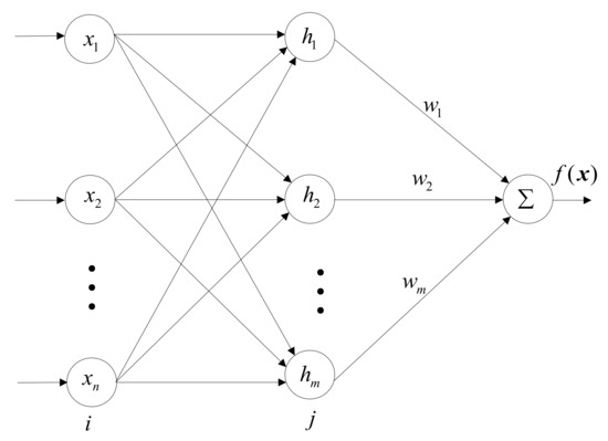
Figure 2.
Structure of RBFNN.
The output of the RBFNN output layer is as follows:
where is the ‘optimal’ weight vector that minimizes among all the estimated values of the weight vector , in which
where is a bounded approximation error; that is, there is a small normal number satisfying inequality .
The performance index of the RBFNN output layer is as follows:
where is desired output.
In RBFNN structure, reasonable selection of hidden layer node center, basis function width, and weight parameters can improve convergence speed and approximation accuracy. According to the gradient descent method, the iterative algorithm of output weight, node center, and node basis function width parameters is as follows:
where is the learning rate, and is the momentum factor.
RBFNN input is , and the output is as follows:
Define error function
where is the estimation error of the weight vector.
Assumption 5.is time-varying and bounded; that is, there is an unknown constant , which satisfies the inequality .
The control law and adaptive law of RBFNN parameters are designed as follows:
where is an adaptive parameter matrix, and is a control parameter.
Theorem 1.
According to the train dynamics model described by Equation (5), under the Assumption of 1–5, an adaptive law (22) for the coefficients of the basic resistance Davis equation, a controller (36) for the system, and an adaptive law (37) for approximating the weight vector of the neural network with additional resistance disturbance are designed. When the Davis equation coefficients are uncertain, the additional resistance disturbance cannot be accurately modeled, the train can track the desired train operation curve in real time, the tracking error converges to a small enough neighborhood quantified by the control parameters, and the closed-loop system is stable. The initial state of the closed-loop system is as follows:
where,is an any positive constant, ,,,and ,are control parameters.
Proof ofTheorem 1.
The Lyapunov function is chosen as
The two sides differential of the is obtained
By substituting the Equations (10), (22), (36), and (37) into Equation (39), we can get
According to Young’s inequality properties, we can get
By substituting Equations (41)–(46) into Equation (40), we can get
Define
Thus
By selecting the appropriate design parameters , , , , and , satisfy . If , then , that is, is an invariant set. If holds, then for , that is .
According to the definition of and Equation (50), we can know is bounded. Thus, closed-loop error signals , , , , , and are bounded, so, , , , and are bounded. According to Equation (50), it can be concluded that
The above inequality (51) means that there is a moment , and for , is always established. According to the definition of , it is easy to know that , , , , , and converge to the following compact sets respectively:
From the above conclusion, it can be seen that the tracking error of the system can be adjusted to any small value by selecting the appropriate design parameters. At the same time, the influence of initial estimation error , , , and on system performance can be adjusted to any small value by selecting appropriate design parameters. Therefore, the introduction of RBFNN to estimate the additional resistance interference in the system will weaken the gain of the switching function to a certain extent to avoid chattering and improve the anti-interference ability of the control system. □
4.3. RBFNN Adaptive Terminal Sliding Mode Fault Tolerant Controller
In the urban rail ATO, the control method without fault-tolerant function is difficult to meet the requirements of high-precision control due to the limit value, delay and fault of many links such as an actuator, speed sensor, and interface equipment. On the one hand, the factors of comfort and the not infinite traction or brake force of the train lead to the input saturation problem; on the other hand, when the speed sensor detects the speed value of the urban rail train and transmits it to the on-board control unit, as well as the on-board software data preprocessing process, there is a time lag in the data transmitted to the on-board control unit. Furthermore, after a long-time high-speed operation of urban rail trains, the traction or brake actuator of the train will inevitably experience mechanical fatigue damage and accumulated wear due to the complicated work, which will lead to traction or brake failures of the train. This puts forward higher requirements for ATO; ATO systems must have adaptive fault tolerance to ensure the safe operation of urban rail trains [33,34].
Considering the faults of the train traction or brake system and physical limitations, the actual control input of the train traction or brake system is usually constrained by scalar function, upper and lower limits; that is, the relationship between and designed control law is as follows:
Design adaptive control law for scalar function
where and are parameters to be designed, and represent the constant of the upper limit value of traction acceleration and the lower limit value of brake deceleration, respectively, and is an estimate of a time-varying scalar function . Scalar function satisfies , which represents the efficiency factor or health index of train traction or brake. means that the train control mechanism can work normally. means that the train control mechanism is completely invalid. means that the train control mechanism is partially invalid. This paper assumes that .
5. Simulation Experiment
In order to verify the effectiveness of the proposed control algorithm, MATLAB 2018a simulation results are given in this paper. The control effects of ATSM-FTC without RBFNN and ATSM-FTC-RBFNN are compared. In the simulation model, the train operating route length is 53.88 km, the train operating time is 2000 s, and the desired position and speed curve of train tracking are shown in Figure 3. The parameter information of train routes such as slope and curve are shown in Table 1.

Figure 3.
Desired speed and position profiles of train operation.

Table 1.
Parameters for route condition.
In the simulation environment, the delay of the speed sensor is set as , the input saturation is quantified as the upper limits of acceleration , and the lower limits of deceleration . The basic resistance simulation parameters are set as , , . The structure of RBFNN is 2-5-1, , . The control parameters are set as , , , , , , , , , , , , , , . When the simulation time is greater than or equal to 5, take . The initial state is selected as , , , , , and .
For the given curve of train desired position and desired speed, Figure 4 and Figure 5 respectively show the performance diagrams of position tracking and speed tracking of ATO control algorithm based on ATSM-FTC-RBFNN. It can be seen from Figure 4 and Figure 5 that the ATSM-FTC-RBFNN algorithm has good tracking performance and can realize high-precision tracking of the desired position and speed curve. According to the enlarged diagram shown in Figure 4, it can be seen that the position tracking error of the control algorithm at the parking point is −2 mm. According to the enlarged diagram shown in Figure 5, when the control algorithm approaches the parking position, the speed tracking error gradually decreases and finally approaches zero. Therefore, the ATSM-FTC-RBFNN control method can achieve high-precision tracking of train desired position and speed curve, and the position signal and speed signal are bounded under the conditions of input saturation limit, speed delay, actuator failure, uncertain Davis equation coefficient of basic resistance, and additional resistance disturbance.
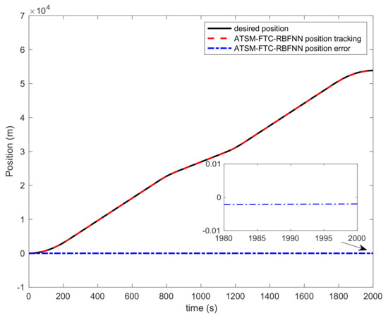
Figure 4.
Position tracking performance ATSM-FTC-RBFNN.

Figure 5.
Speed tracking performance of ATSM-FTC-RBFNN.
As shown in Figure 6, the position error of ATSM-FTC-RBFNN is the largest when the train is just started. With the normal operation of the train for 630 s, the position tracking error is reduced to zero. In the process of train operation, due to the influence of the uncertainty of Davis equation coefficient of basic resistance and the interference of route additional resistance, the position tracking error increases negatively to −0.155 m in 1148 s, and then increases continuously. After 96 s, the position error increases to 0.13 m and then decreases continuously. The final parking accuracy is −2 mm. Although the position tracking error of train operation changes continuously, the position control accuracy at any time is less than ±0.2 m, which meets the requirements of accurate train control.

Figure 6.
Position error of ATSM-FTC-RBFNN.
As shown in Figure 7, the overall speed error of ATSM-FTC-RBFNN is −0.04~0 m/s, which does not exceed the desired speed, ensuring the safety of train operation. When the train operates to 1148 s, the control accuracy of the ATSM-FTC-RBFNN controller is reduced due to the sudden change of desired speed, the uncertainty of Davis equation coefficient of basic resistance, and the interference of route additional resistance, and the speed error is −0.06 mm. In order to overcome the mutation, uncertainty, and disturbance of the outside condition, the controller enhances the discontinuous nonlinear switching control in this period to maintain the control accuracy, as shown in Figure 8, which not only ensures the stable operation of the train on the route under the influence of various factors and disturbances, but also the final speed control error is close to zero.
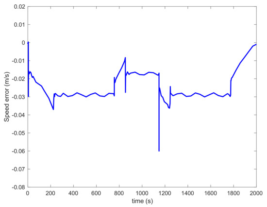
Figure 7.
Speed error of ATSM-FTC-RBFNN.
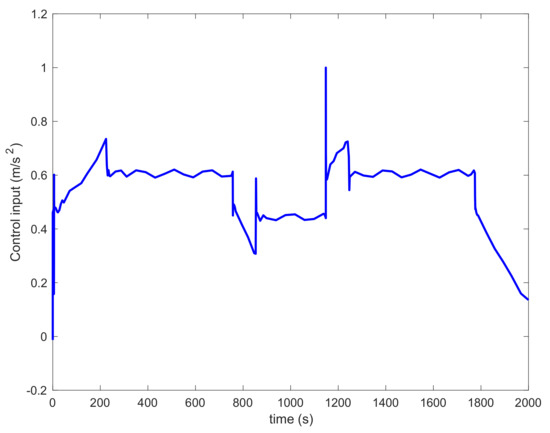
Figure 8.
Control input of ATSM-FTC-RBFNN.
For the given curve of train desired position and desired speed, Figure 9 and Figure 10 respectively show the performance diagrams of position tracking and speed tracking of the ATO control algorithm based on ATSM-FTC. It can be seen from Figure 9 and Figure 10 that the ATSM-FTC algorithm can track desired position and speed curve. According to the enlarged diagram shown in Figure 9, the position tracking error of the control algorithm at the parking point is −0.42 m. According to the enlarged diagram shown in Figure 10, when the control algorithm is close to the parking position, the speed tracking error is almost zero. Therefore, the ATSM-FTC control method can basically meet the control requirements of the given train position and speed curve tracking under the conditions of input saturation limit, speed delay, actuator failure, uncertain Davis equation coefficient of basic operating resistance, and additional operating resistance disturbance.

Figure 9.
Position tracking performance of ATSM-FTC.
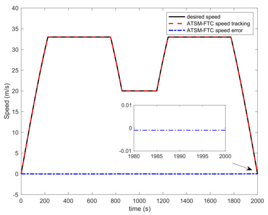
Figure 10.
Speed tracking performance of ATSM-FTC.
As shown in Figure 11, the position tracking error of ATSM-FTC is −0.4~0.42 m. In the process of train operation, the position tracking error and speed tracking error have fluctuations due to the influence of train performance and external interference. The speed tracking error of ATSM-FTC is shown in Figure 12, which is between −0.11 and 0.02 m/s. When the train just starts, it exceeds the expected speed by 0.02 m/s. After the train operates normally, its speed does not exceed the given desired speed. However, when the train operates between 846 and 1148 s, the control accuracy of the ATSM-FTC controller decreases due to the sudden change of desired speed and the influence of the operation environment. In order to overcome the mutation and influence of the outside environment, the controller enhances the nonlinear switching control in this period to maintain the control accuracy, as shown in Figure 13.
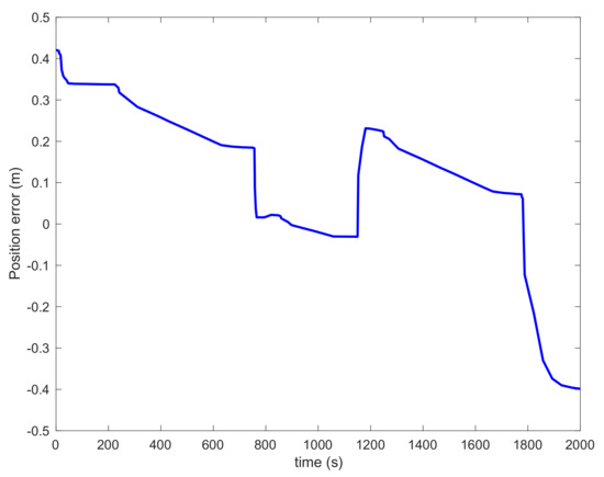
Figure 11.
Position error of ATSM-FTC.
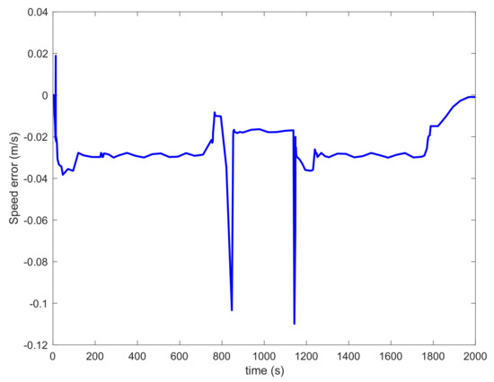
Figure 12.
Speed error of ATSM-FTC.
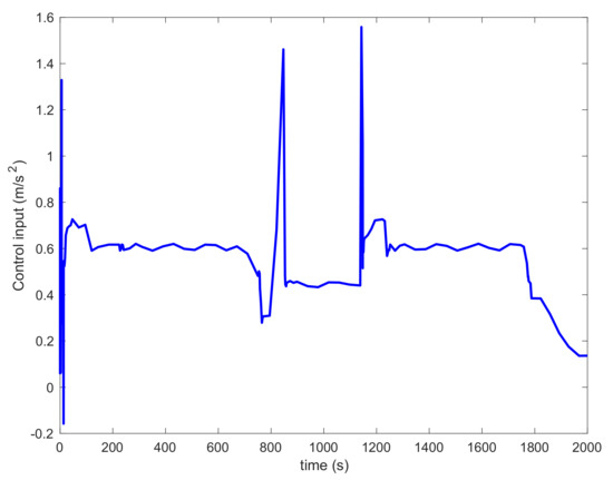
Figure 13.
Control input of ATSM-FTC.
In order to further explore the performance of the controller, ATSM-FTC-RBFNN controller, ATSM-FTC controller, MFAC, and MFA-FTC controller in reference [17] are used for comparison. The actuator fault coefficient in reference [17] is shown in Table 2. In addition, in [17], the parameter settings of RBFNN remain unchanged, and the remaining parameters of the controller are set as , , , , , , , , and .
Table 2.
Actuator failure factor table.
Figure 14, Figure 15 and Figure 16 show the simulation comparison results of four controllers. Figure 14 is the position tracking error of the four controllers; Figure 15 is the speed tracking error of the four controllers; and Figure 16 is the control input of the four controllers. It can be seen from Figure 14 and Figure 15 that when facing external interference, the ATSM-FTC-RBFNN controller has fast adjustment speed, fast convergence of the whole process state, strong anti-disturbance ability, good control performance, and strong fault tolerance, and can ensure the safe and reliable operation of the train. When the ATSM-FTC control is faced with external interference, its state error converges slowly. That is to say, in the whole process of train operation, the position error and speed error of the train are large. The position tracking error and speed tracking error of the MFAC controller in reference [17] gradually diverge with the increase of fault degree, and the tracking performance is significantly reduced. Compared with MFAC, the position tracking error and speed tracking error of the MFA-FTC control algorithm in [17] are significantly improved. But when the degree of external interference and fault is large, there will be large oscillations, and the fault-tolerant control performance is poor.

Figure 14.
Position error comparison.
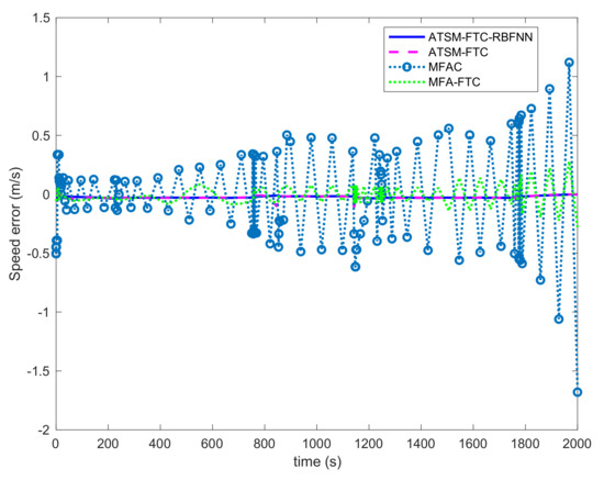
Figure 15.
Speed error comparison.
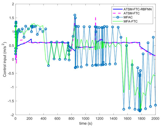
Figure 16.
Control input comparison.
It can be seen from Figure 16 that the train needs to overcome its own gravity and other resistance when it just starts, and the control input value is relatively large. After the train operates normally, the control input of ATSM-FTC-RBFNN controls the train with small fluctuations, and the train operates the most smoothly, which meets the comfort requirements of passengers. Although the overall oscillation amplitude of ATSM-FTC is relatively small, large oscillations occur at both 846 and 1148 s when the external disturbance is large, which affects the fault-tolerant performance. The control input of the MFAC and MFA-FTC controllers in [17] has large oscillations. Compared with MFAC, the oscillation amplitude of MFA-FTC has been improved, but the constantly changing control input will increase the traction and brake switching times. The number of times shortens the service life of the actuator, and it is also not conducive to safe driving. It can be seen that the ATSM-FTC-RBFNN controller has better system dynamic response quality, optimal adaptive control performance, and strong anti-disturbance and fault tolerance capabilities.
In order to better investigate the control performance of the ATSM-FTC-RBFNN control algorithm, a simulation test is carried out for the uncertainty of the model parameters of the controller. The parameters of the train model were changed within the range of ±10%, and the simulation experiment of 100 times train operations and precise parking was performed. The simulation results are shown in Table 3. It can be seen from Table 3 that the control algorithm for the train dynamics model with random changes in model parameters, the control effect is still good, and the position errors are all within 0.2 m, of which 70% are within 0.1 m. The simulation results show that the ATSM-FTC-RBFNN control algorithm can synchronously compensate and deal with the nonlinear effects of control input saturation, time delay, actuator failure, etc. It can adapt to changes in train control system model parameters and has good robustness and anti-interference.
Table 3.
Position error distribution condition.
6. Discussion
One of the most important functions of ATO is to control the train to accurately track the speed curve according to different train models and operating conditions (such as tunnels, curves, and steep slopes) so that the train can run safely and smoothly. The most widely used control method in ATO is PID controller (such as Beijing Metro Yizhuang Line, Changping Line, etc.) and the combination of PID and other intelligent control, such as fuzzy PID [35], sliding mode PID [36], RBF neural network PID [37], etc. Although the controller based on PID can obtain better tracking performance in the practical application of ATO, the ride comfort based on PID controller is poor due to the frequent switching of PID control commands. In addition to the mainstream PID control, other research on ATO control algorithms can be divided into two categories. One is the ATO controller designed by using train dynamics model information to ensure the accuracy of curve tracking, which is called model-based control method in this paper. The second category is to use the input and output data generated during train operation to estimate the system parameters online so as to realize the model-free adaptive control of the train, which is called the model-free adaptive control method in this article. The model-free adaptive control method only establishes the connection between the input and output data of the system, and does not have a clear physical meaning. It cannot predict and analyze the train dynamic behavior based on the dynamic input and output data model. For the straight routes, this method can track the position and speed curve with less error, but for the train operation environment with large external interference, the current model-free adaptive control method is difficult to ensure a consistent train operation control performance index for a long time, which needs to be further improved.
Model-based control methods include single-particle dynamics models and multi-particle dynamics models. Since train dynamics is related to multiple factors, it is too complicated to establish a multi-particle dynamics model that can describe many factors, such as describing seven cars dynamics requires 84 differential equations [38]. The overly complex models are not conducive to the design of ATO controllers. Therefore, the mainstream research on the ATO control algorithm is based on the single-particle dynamics model. The research on the ATO control method in this paper is based on the single-particle train dynamics model. The establishment of the train dynamics model is an important part of ATO controller design. The accuracy of the model is directly related to the controller design and control effect. The dynamic behavior of train motion is related to many factors. It is very difficult to establish an accurate model. Besides its own traction and braking force, it is also affected by a variety of external and internal forces, including bearing friction resistance, wheel rolling and sliding resistance, impact and vibration resistance, air resistance, ramp resistance, curve resistance, tunnel resistance, etc. However, for different models, routes, and even different weather conditions, the model parameters will change, resulting in the uncertainty of the system model parameters. Therefore, it is necessary to design an adaptive control strategy that can identify unknown parameters and ensure good convergence. It is the first step to study the ATO control algorithm. The automatic train operating process also needs to consider multiple performance goals, namely energy consumption, punctuality, and ride comfort. In addition, under the long-term high-speed operation of urban rail trains, the traction or braking mechanism of the train is prone to failure due to factors such as high-temperature friction and severe vibration. Therefore, the fault-tolerant ability should also be considered in the design of the ATO system to ensure the operation safety of urban rail trains.
Combining the above contents, this paper comprehensively considers the uncertainty of the train dynamics model, multiple train performance indicators, and fault tolerance and proposes the ATSM-FTC-RBFNN control algorithm, which is compared with [17]. In contrast, the ATSM-FTC-RBFNN control algorithm has better control effects, can adapt to the changes in train parameters, can well overcome external interference, and can ensure higher control accuracy. At the same time, it effectively reduces the chattering caused by sliding mode control, improves the robustness and dynamic characteristics of the controller, and has a wide range of practicability.
7. Conclusions
Taking the automatic train driving system of urban rail as the research object, the precise control algorithm of urban rail trains is studied in this paper. Combined with the train dynamics model, the mathematical description of the train control process is given. Aiming at the precise control technology in automatic train operation, an adaptive terminal sliding mode controller is proposed. The terminal sliding mode control is used to design the control algorithm, and the parameter adaptive mechanism is introduced to enhance the control system adaptability. Based on the ATO algorithm of adaptive terminal sliding mode control, the RBFNN disturbance approximator is designed, and the disturbance value of the RBFNN disturbance approximator is introduced into the control algorithm to enhance the robustness and anti-disturbance ability of the system. At the same time, the problem of input saturation caused by train traction or braking force cannot be infinite, the transmission delay of speed sensor and the partial failure of traction or braking actuator in ATO system are considered, and the fault-tolerant mechanism is introduced. The simulation results show that when the model has parameter uncertainty and external disturbance, the designed control algorithm can synchronously compensate and deal with the nonlinear effects such as control input saturation, time delay, and actuator failure to ensure the accurate control of train operation.
Combined with the research content of this paper, the future work that should be carried out in-depth research is as follows:
- Research on the optimization strategy and control method of automatic train operation based on deep learning and knowledge automation. In this paper, from the perspective of mechanism modeling, the train dynamics model is obtained by analyzing the force of the train. However, the massive data generated during the actual operation of the train is not fully utilized and excavated. Mining rules from historical data and accurate prediction will help to grasp the train operation status in detail and provide more decision support for the dispatching command;
- Research on the optimization strategy and control method of multi-train intelligent operation for multi-train cooperative operation. Under the conditions of high-density and long-period operation of urban rail trains, multi-train collaborative control is a solution to achieve global optimization and ensure system performance. The development of advanced train-to-train communication, virtual marshalling, and other technologies and their application in multi-train operation control systems are the development trend and inevitable trend in recent years.
Author Contributions
Conceptualization, J.Y. and Y.Z.; Data curation, J.Y.; Formal analysis, J.Y.; Investigation, J.Y., Y.Z. and Y.J.; Methodology, J.Y.; Project administration, Y.Z.; Resources, J.Y., Y.Z. and Y.J.; Software, J.Y.; Supervision, Y.Z.; Validation, Y.J.; Visualization, Y.Z. and Y.J.; Writing—original draft, J.Y.; Writing—review & editing, J.Y. All authors have read and agreed to the published version of the manuscript.
Funding
This research was funded by NSFC, Grant No. 61963023.
Institutional Review Board Statement
Not applicable.
Informed Consent Statement
Not applicable.
Data Availability Statement
Data sharing not applicable.
Conflicts of Interest
The authors declare no conflict of interest.
References
- Gao, C.H. Rail train operation control system based on communication. Mod. Urban Transit. 2007, 2, 7–10. [Google Scholar]
- Gao, C.H. Study on ATO braking model identification based on model selection and optimization techniques. J. China Railw. Soc. 2011, 33, 56–60. [Google Scholar]
- Yin, J.; Tang, T.; Yang, L. Research and development of automatic train operation for railway transportation systems: A survey. Transp. Res. Part C Emerg. Technol. 2017, 85, 548–572. [Google Scholar] [CrossRef]
- Dong, H.R.; Gao, S.G.; Ning, B. Extended fuzzy logic controllers for high speed train. Neural Comput. Appl. 2013, 22, 321–328. [Google Scholar] [CrossRef]
- Shi, W.S. Research on automatic train operation based on model-free adaptive control. J. China Railw. Soc. 2016, 38, 72–77. [Google Scholar]
- Wang, C.; Tang, T.; Luo, R.S. Study on iterative learning control in automatic train operation. J. China Railw. Soc. 2013, 35, 49–52. [Google Scholar]
- Yu, J.; Qian, Q.Q.; He, Z.Y. Genetic algorithms with application to optimize high speed train ATO. Am. Soc. Civ. Eng. 2007, 2007, 2512–2517. [Google Scholar]
- Wang, Y.H.; Luo, R.S.; Yu, Z.Z. Study on ATO control algorithm with consideration of ATP speed limits. J. China Railw. Soc. 2018, 34, 59–64. [Google Scholar]
- Luo, R.S.; Wang, Y.H.; Yu, Z.Z. Adaptive stopping control of urban rail vehicle. J. China Railw. Soc. 2016, 34, 64–68. [Google Scholar]
- Luo, H.Y. Study on model reference adaptive control of ATO systems. J. China Railw. Soc. 2018, 35, 69–73. [Google Scholar]
- He, Z.Y.; Xu, N. Automatic train operation algorithm based on adaptive iterative learning control theory. J. Transp. Syst. Eng. Inf. Technol. 2020, 20, 69–75. [Google Scholar]
- Cao, Y.; Zhang, Y.Z. Application of fuzzy predictive control technology in automatic train operation. Clust. Comput. 2018, 22, 78–85. [Google Scholar] [CrossRef]
- Song, Q.; Song, Y.D. Data-based fault-tolerant control of high-speed trains with traction/braking notch nonlinearities and actuator failures. IEEE Trans. Neural Netw. 2011, 22, 2250–2261. [Google Scholar] [CrossRef]
- Li, Z.; Hou, Z.; Yin, C. Iterative learning control for train trajectory tracking under speed contains with iteration-varying parameter. Trans. Inst. Meas. Control 2015, 37, 485–493. [Google Scholar] [CrossRef]
- Gao, S.G.; Dong, H.R.; Ning, B. Adaptive fault-tolerant automatic train operation using RBF neural networks. Neural Comput. Appl. 2015, 26, 141–149. [Google Scholar] [CrossRef]
- Zhang, R.K. Adaptive iterative learning control for high-speed trains with unknown speed delays and input saturations. IEEE Trans. Autom. Sci. Eng. 2016, 13, 260–273. [Google Scholar]
- Wang, H.J. Model-free adaptive fault-tolerant control for subway trains. Beijing Jiaotong Univ. 2020, 14, 30–46. [Google Scholar]
- Park, K.B.; Tsuiji, L. Terminal sliding mode control of second-order nonlinear uncertain systems. J. Robust Nonlinear Control. IFAC Affil. J. 1999, 9, 769–780. [Google Scholar] [CrossRef]
- Wang, J.; Zhao, L.; Yu, L. Adaptive terminal sliding mode control for magnetic levitation systems with enhanced disturbance compensation. IEEE Trans. Ind. Electron. 2020, 11, 11–23. [Google Scholar] [CrossRef]
- Schilling, R.J.; Carroll, J.J.; Al-Ajlouni, A.F. Approximation of nonlinear systems with radial basis function neural networks. IEEE Trans. Neural Netw. 2001, 11, 423–429. [Google Scholar] [CrossRef] [Green Version]
- Ghosh, D.S.; Adeli, H.; Dadmehr, N. Principal component analysis-enhanced cosine radial basis function neural network for robust epilepsy and seizure detection. IEEE Trans. Biomed. Eng. 2008, 55, 512–518. [Google Scholar] [CrossRef]
- Leung, H.; Lo, T.; Wang, S. Prediction of noisy chaotic time series using an optimal radial basis function neural network. IEEE Trans. Neural Netw. 2016, 12, 1163–1172. [Google Scholar] [CrossRef] [PubMed]
- Fu, D.X.; Zhao, X.M. Backstepping terminal sliding mode control based on radial basis function neural network for permanent magnet linear synchronous motor. Trans. China Electrotech. Soc. 2020, 35, 2354–2546. [Google Scholar]
- Meng, Z.; Tang, T.; Wei, G. Analysis of ATO system operation scenarios based on UPPAAL and the operational design domain. Electronics 2021, 10, 503. [Google Scholar] [CrossRef]
- Wang, L.; Wang, X.; Sheng, Z. Multi-objective shark smell optimization algorithm using incorporated composite angle cosine for automatic train operation. Energies 2020, 13, 714. [Google Scholar] [CrossRef] [Green Version]
- Wang, Q.Y.; Wu, P.; Feng, X.Y. Precise automatic train stop control algorithm based on adaptive terminal sliding mode control. J. China Railw. Soc. 2016, 38, 56–63. [Google Scholar]
- Meng, J.; Xu, R.; Li, D. Combining the matter-element model with the associated function of performance indices for automatic train operation algorithm. IEEE Trans. Intell. Transp. Syst. 2019, 20, 253–263. [Google Scholar] [CrossRef]
- Davis, W.J. The tractive resistance of electric locomotives and cars. Gen. Electr. 1926, 2, 26–32. [Google Scholar]
- Chen, C.L.P.; Liu, Y.; Wen, G. Fuzzy neural network-based adaptive control for a class of uncertain nonlinear stochastic systems. IEEE Trans. Cybern. 2014, 44, 583–593. [Google Scholar] [CrossRef]
- Utkin, V.I.; Yang, K.D. Methods for constructing discontinuity planes in multidimensional variable structure systems. Autom. Remote Control 1978, 10, 72–77. [Google Scholar]
- Broomhead, D.S.; Lowe, D. Radial basis functions, multi-variable functional interpolation and adaptive networks. Complex Syst. 1988, 2, 321–355. [Google Scholar]
- Park, J.; Sandberg, I.W. Universal approximation using radial-basis-function networks. Neural Comput. 1991, 3, 246–257. [Google Scholar] [CrossRef]
- Mao, Z.; Gang, T.; Jiang, B. Adaptive compensation of traction system actuator failures for high-speed trains. IEEE Trans. Intell. Transp. Syst. 2017, 18, 2950–2963. [Google Scholar] [CrossRef]
- Song, Q.; Song, Y.D.; Tang, T. Computationally inexpensive tracking control of high-speed trains with traction/braking saturation. IEEE Trans. Intell. Transp. Syst. 2011, 12, 1116–1125. [Google Scholar] [CrossRef]
- Liu, Y. Optimized research of ATO based on fuzzy self-adaptive PID. Electron. Meas. Technol. 2013, 2, 35–44. [Google Scholar]
- Yang, Y.F.; Cui, K.; Lu, X.J. Combined sliding mode and PID control of automatic train operation system. J. China Railw. Soc. 2014, 36, 61–67. [Google Scholar]
- Wei, W.; Dong, Y. Optimization of train ATO system based on RBF neural network PID Control. In Proceedings of the 5th International Conference on Electromechanical Control Technology and Transportation (ICECTT), Nanchang, China, 15–17 May 2020; pp. 147–239. [Google Scholar]
- Goodall, R.; Kortum, W. Mechatronic developments for railway vehicles of the future. Control Eng. Pract. 2002, 10, 887–898. [Google Scholar] [CrossRef]
Publisher’s Note: MDPI stays neutral with regard to jurisdictional claims in published maps and institutional affiliations. |
© 2021 by the authors. Licensee MDPI, Basel, Switzerland. This article is an open access article distributed under the terms and conditions of the Creative Commons Attribution (CC BY) license (https://creativecommons.org/licenses/by/4.0/).