
Optimal Fractional PID Controller for Buck Converter Using Cohort Intelligent Algorithm


Abstract
:1. Introduction
2. System Description
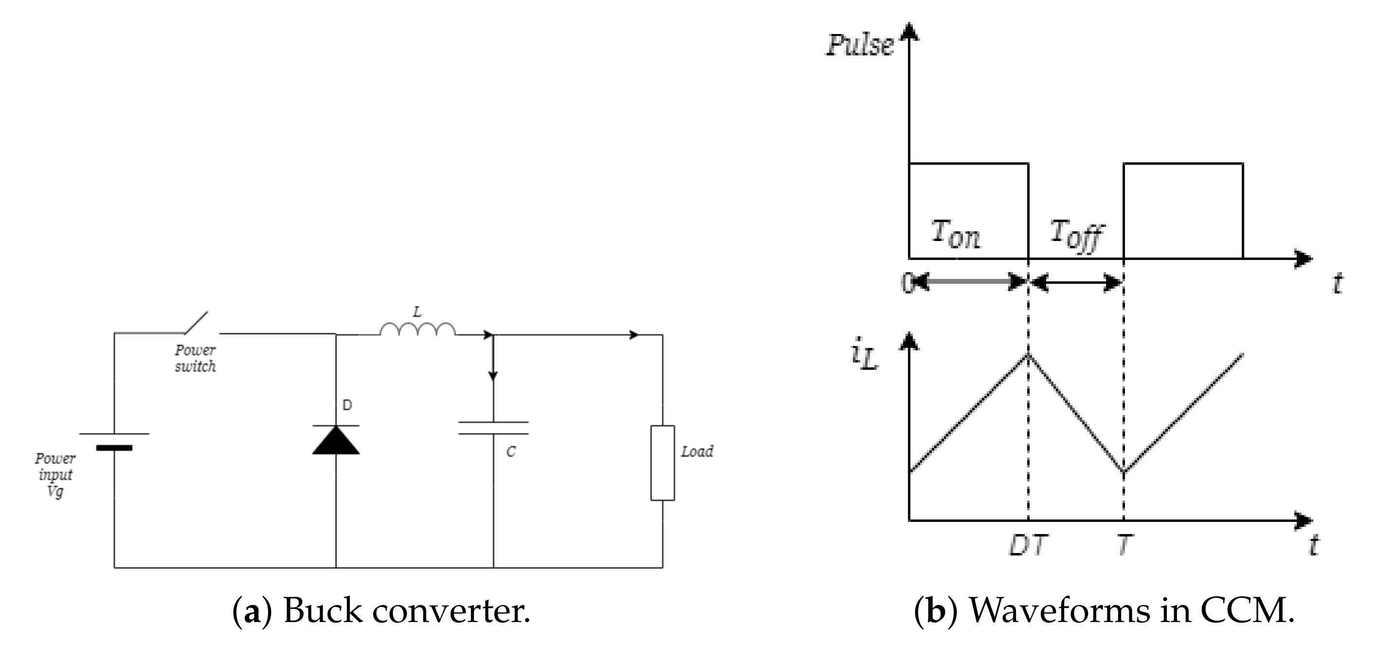
2.1. Buck Converter
2.2. Fractional Order Systems
2.3. Approximation
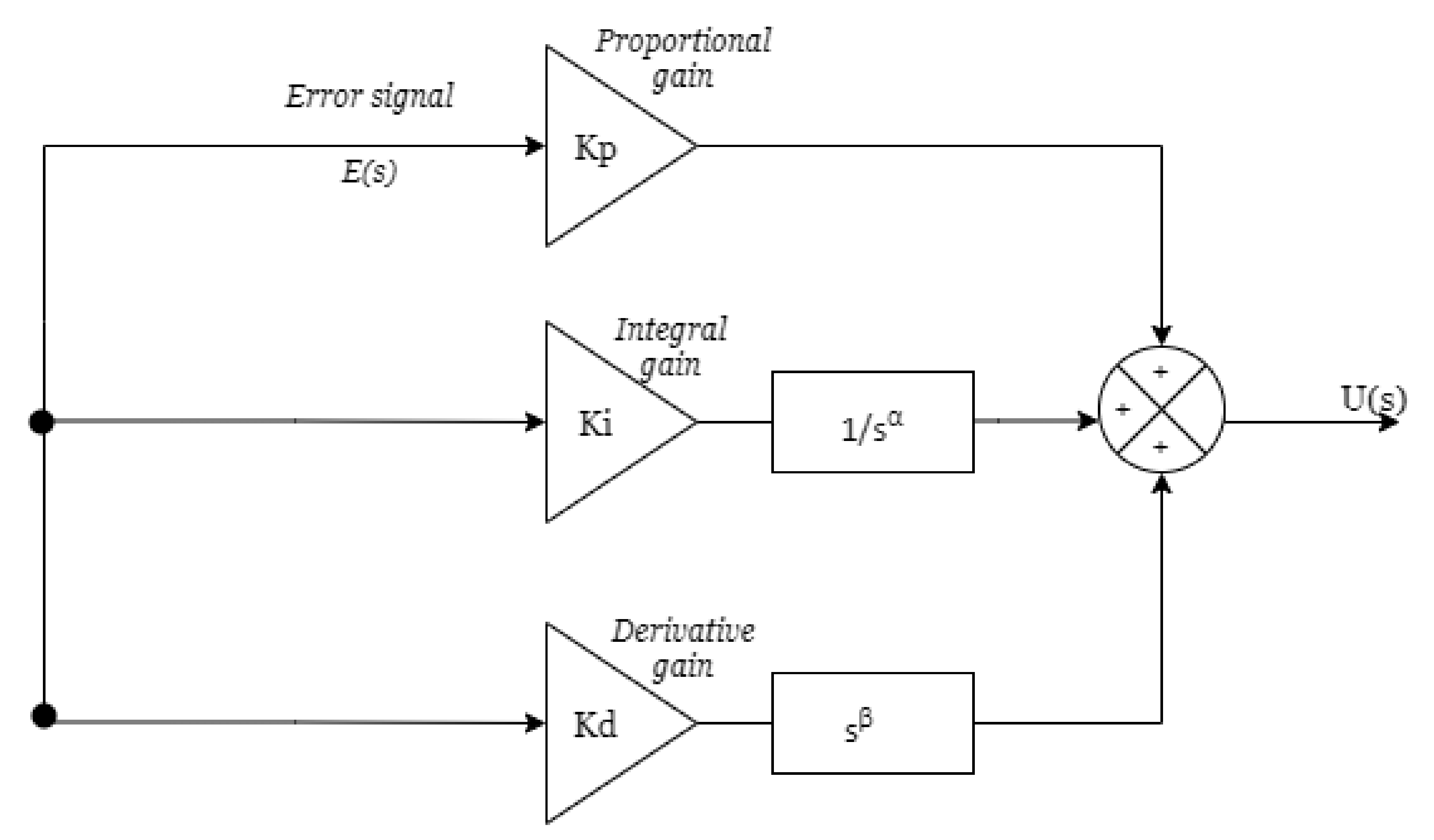
2.4. Fractional PID Control
2.5. CI Algorithm
- Best rule;
- Better rule;
- Worst rule;
- Itself rule;
- Median rule;
- Roulette wheel selection;
- Alienation-and-random selection.
3. Methodology
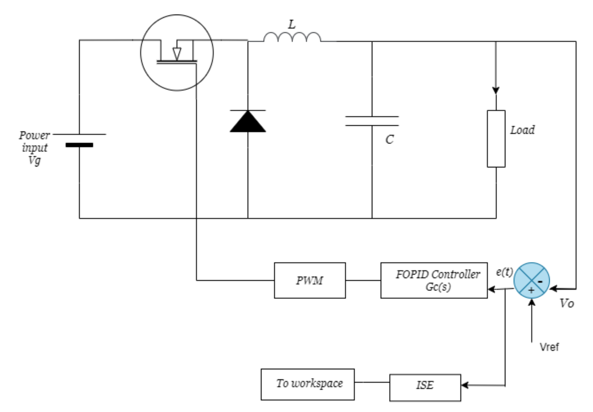
3.1. Optimal Tuning of the Fopid Controller for a Buck Converter
3.2. System Description
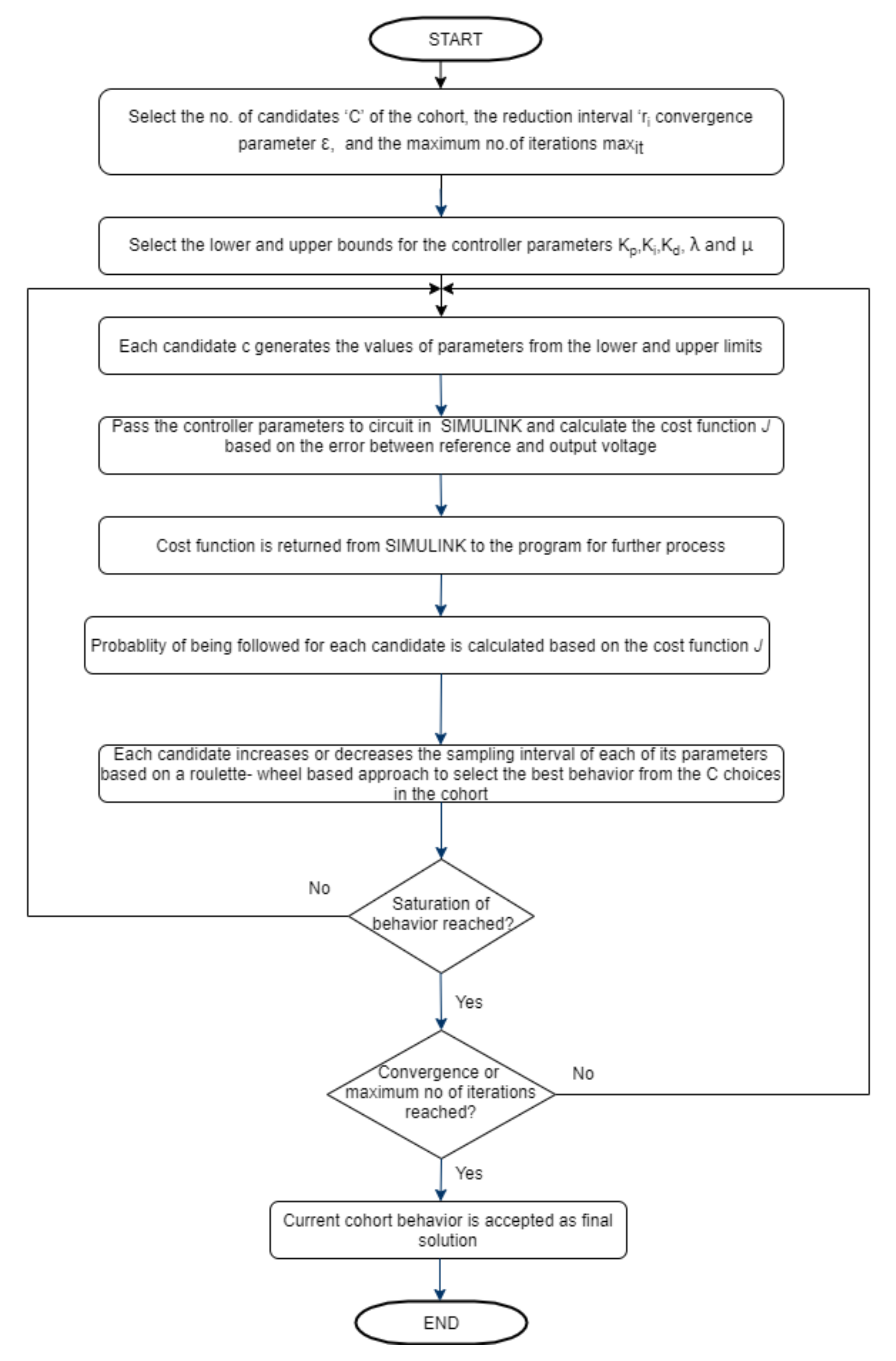
- Select the no. of candidates ‘C’ of the cohort, the reduction interval ‘’, convergence parameter , and the maximum no.of iterations ;
- The lower bound and upper bound of the controller parameters , , , and are chosen based on some initial runs of the algorithm;
- For each candidate c in the cohort, the qualities (parameters and ) are generated from the lower and upper bounds as:where rand is a random number between 0 and 1. Similarly, the values for , , etc., are generated;
- The overall behavior (J) of each candidate is calculated from the error, as given by Equation (9) (in this case);
- The probability function for each candidate is calculated as:
- A roulette wheel approach is used by each candidate to follow another candidate’s behavior. This approach uses one generation as the basis of the next generation. The best solution has the highest probability of being followed;
- Accordingly, each candidate adjusts its sampling interval as shown below for :Similarly, the other four parameters also are adjusted;
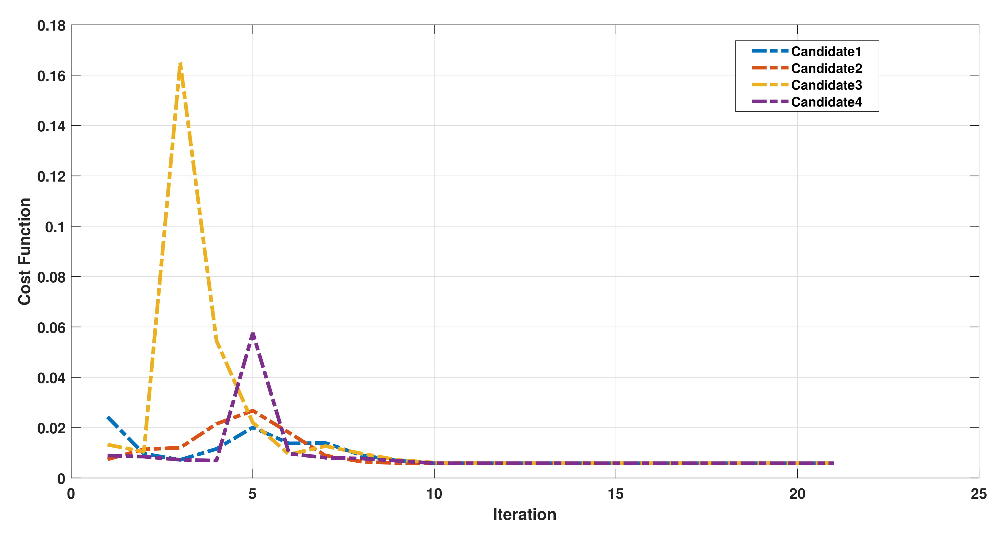
- This process continues till the value of J reaches a saturation condition defined as:
- If the maximum limit of iterations is exceeded or the saturation condition defined in step 8 is reached, then the algorithm terminates. The final solution for the objective function can be accepted from any one of the C behaviors;
- If conditions of steps 8 or 9 are not satisfied, jump to step 3.
4. Results and Discussion
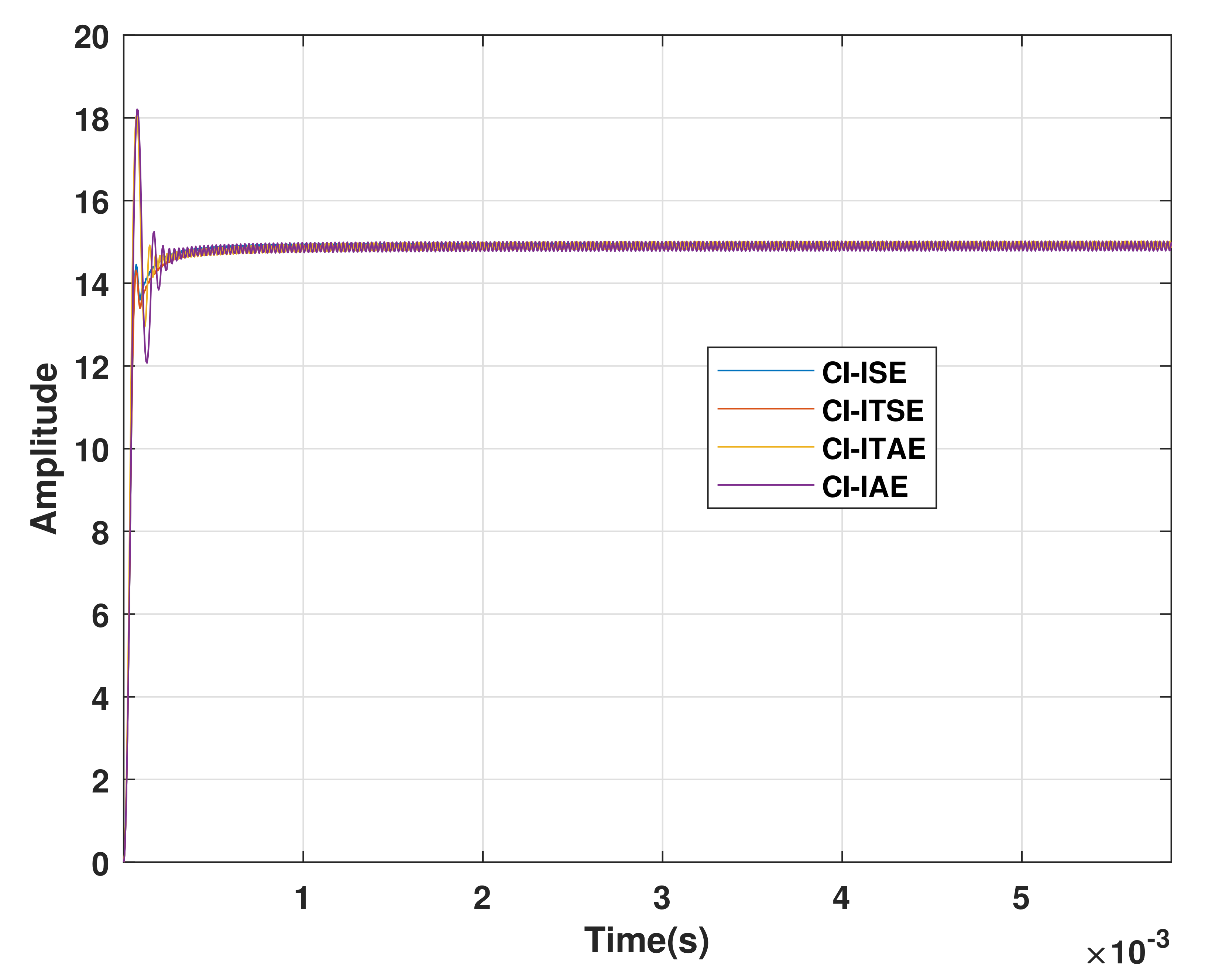
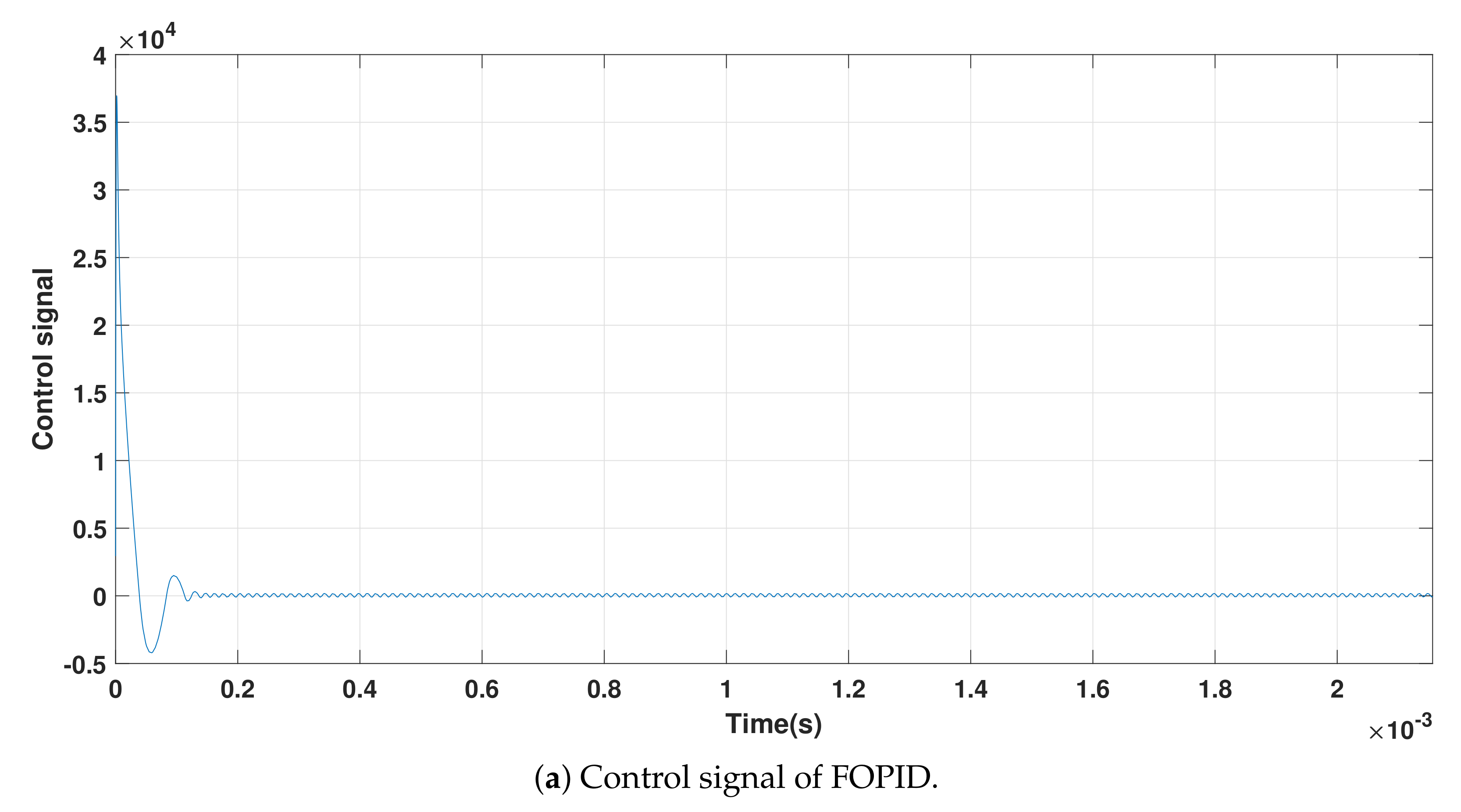
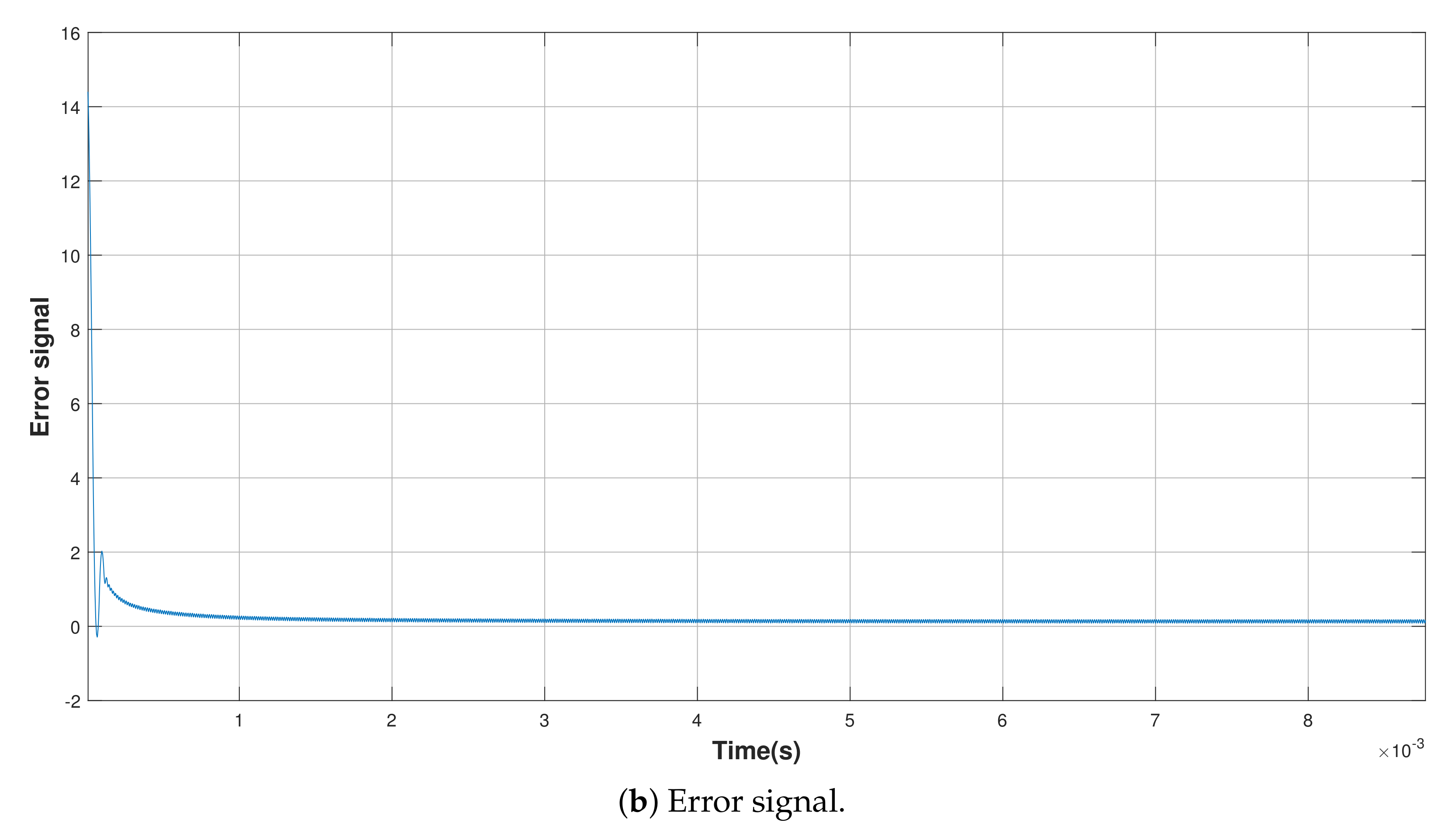
4.1. Start-up Response of the Buck Converter
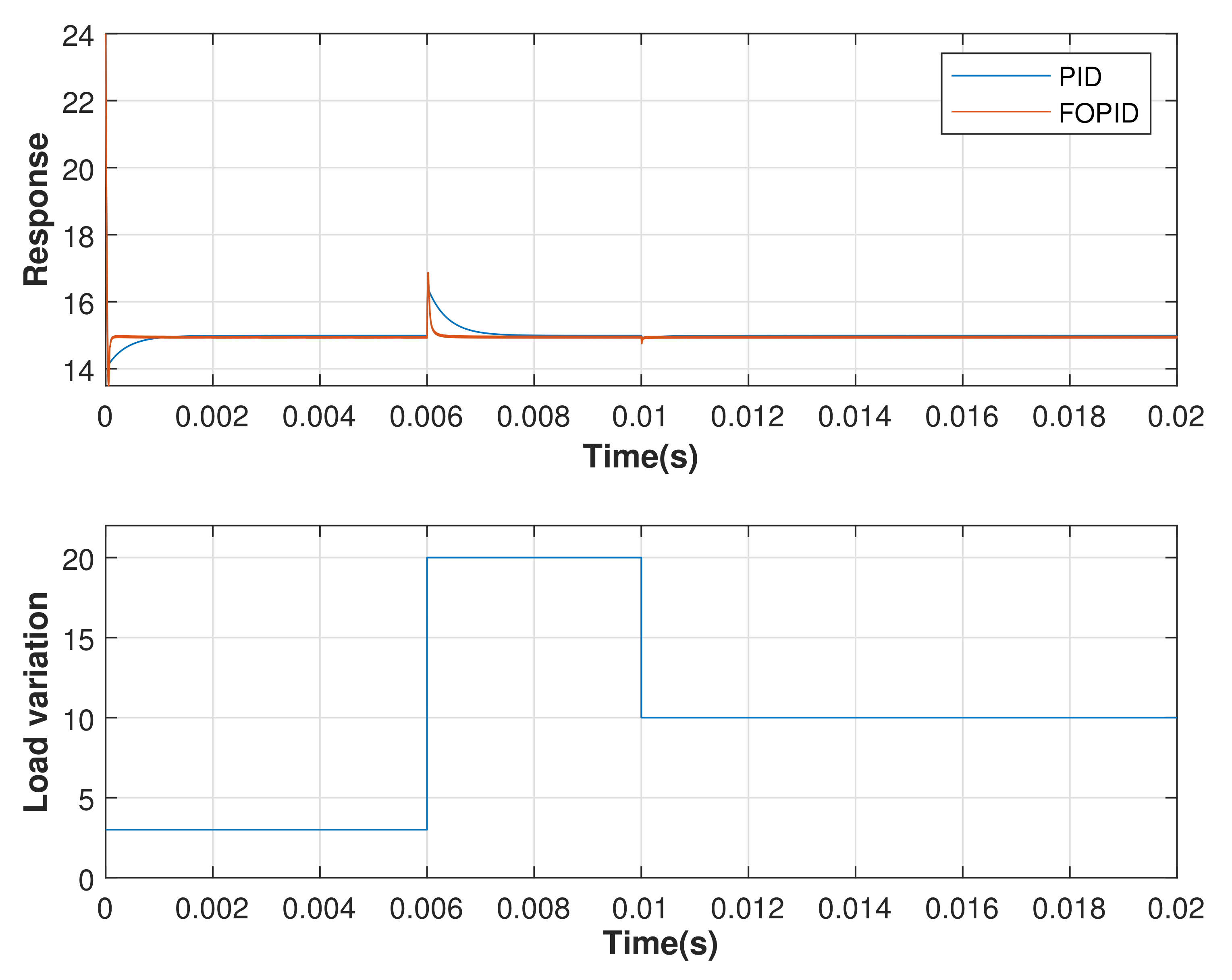
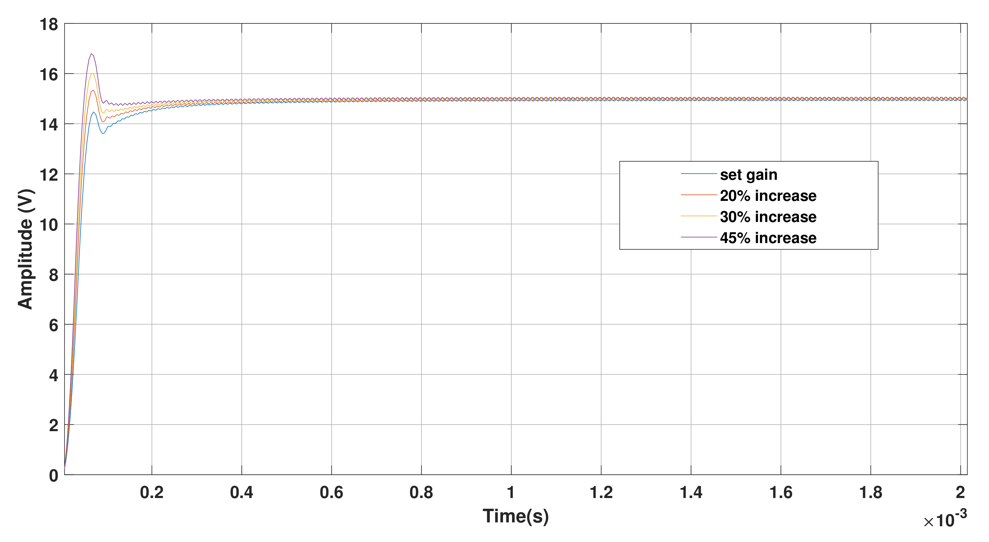
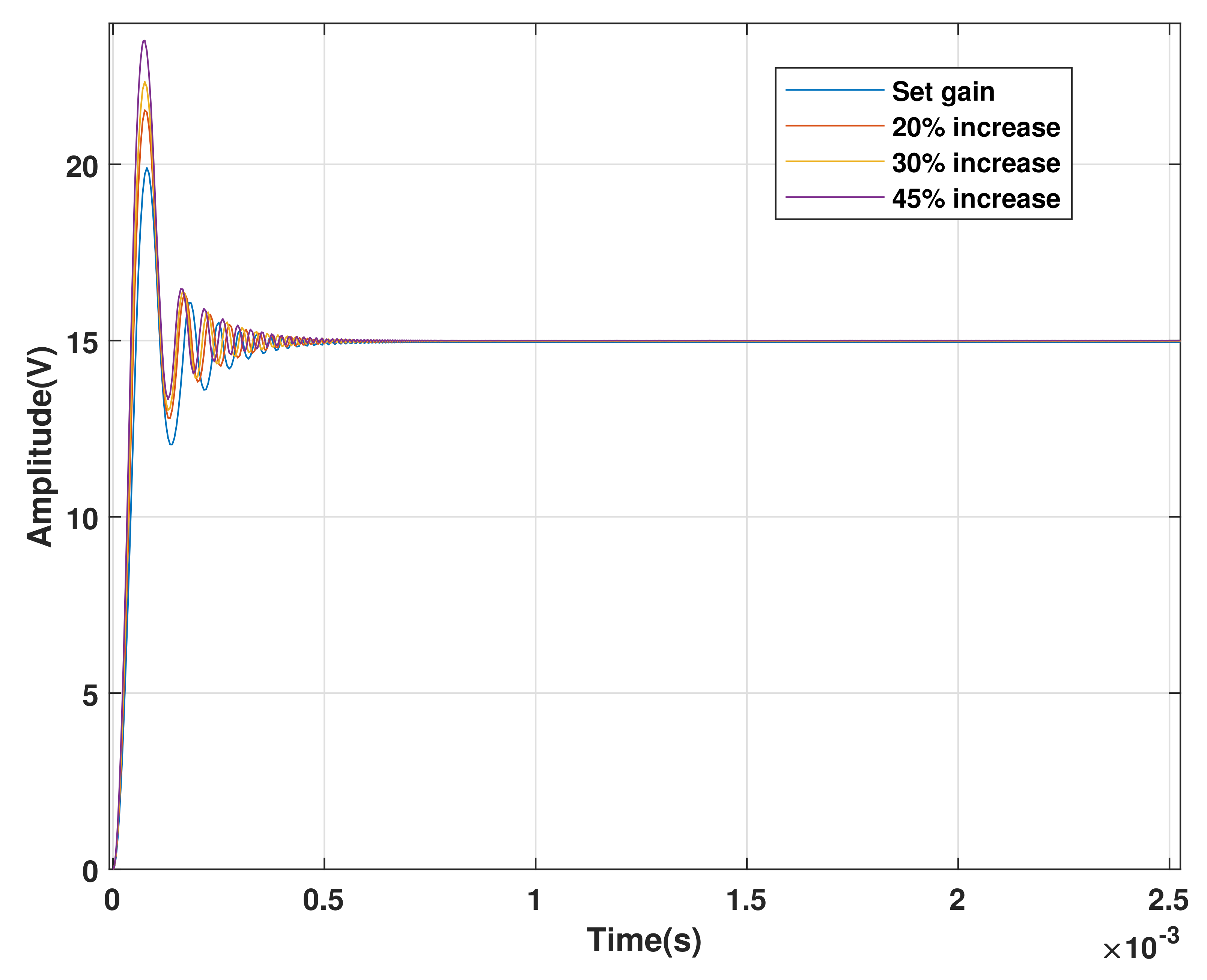
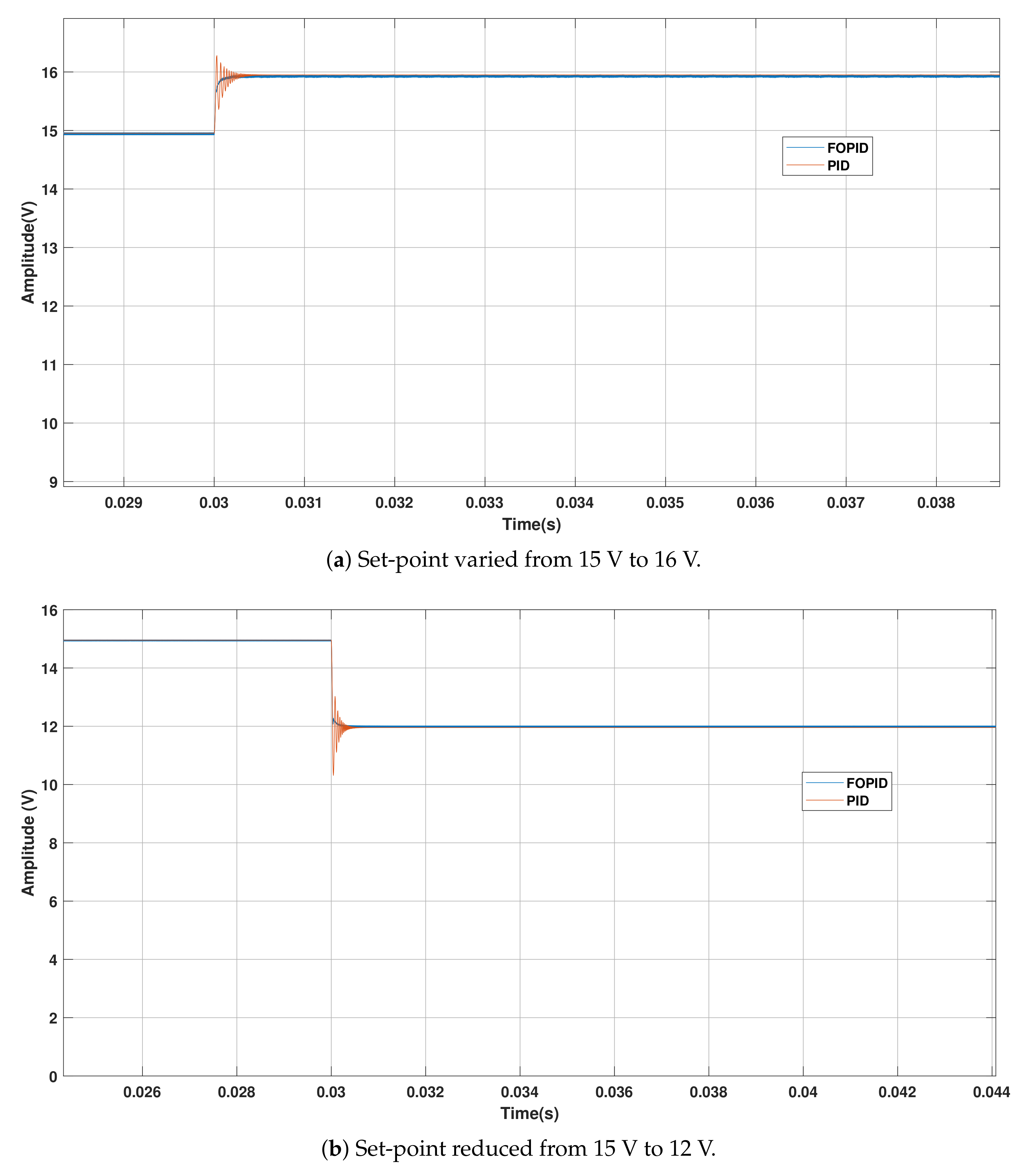
4.2. Response of the CI-Optimized System to DC Gain Variations and Dynamic Changes
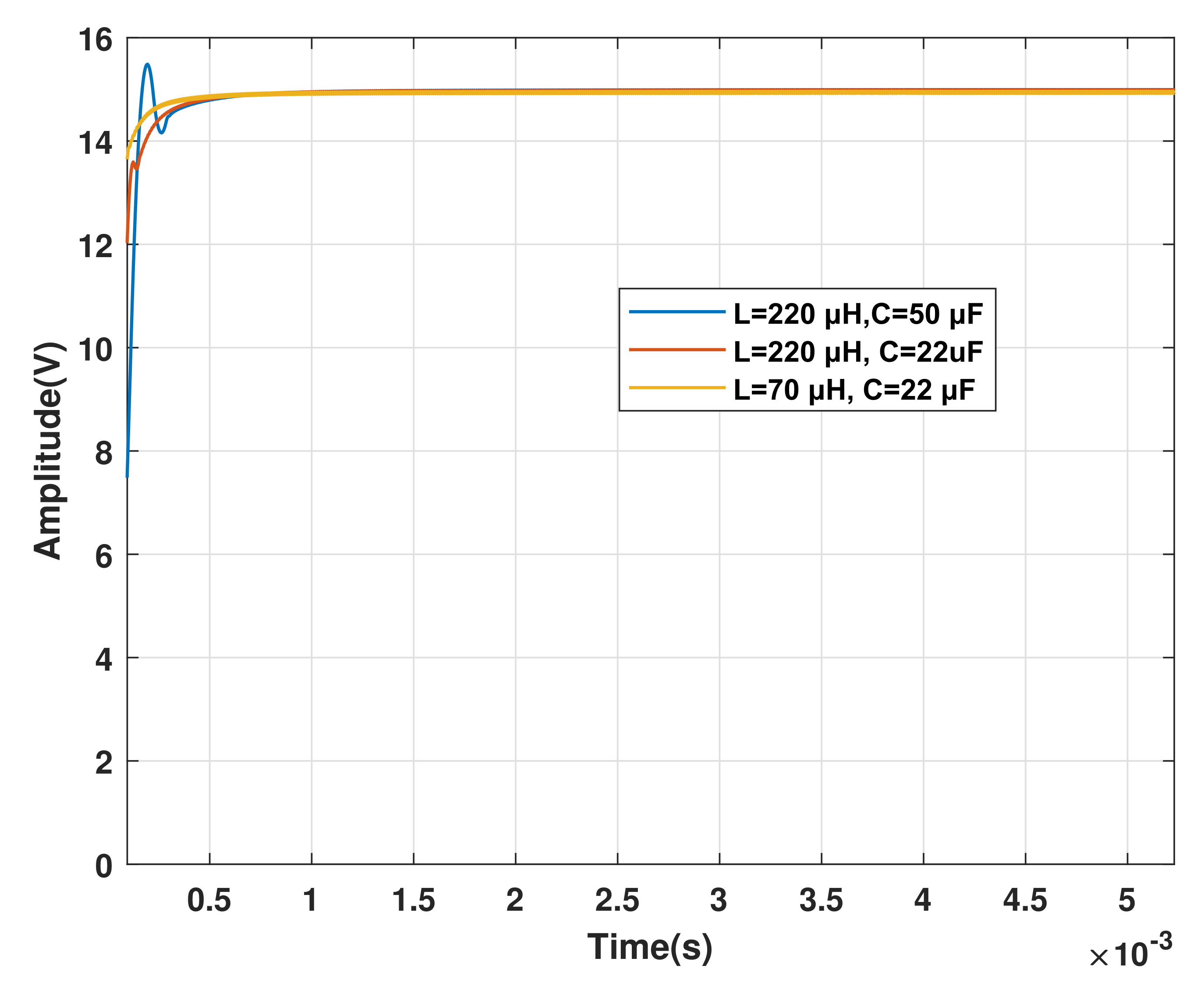
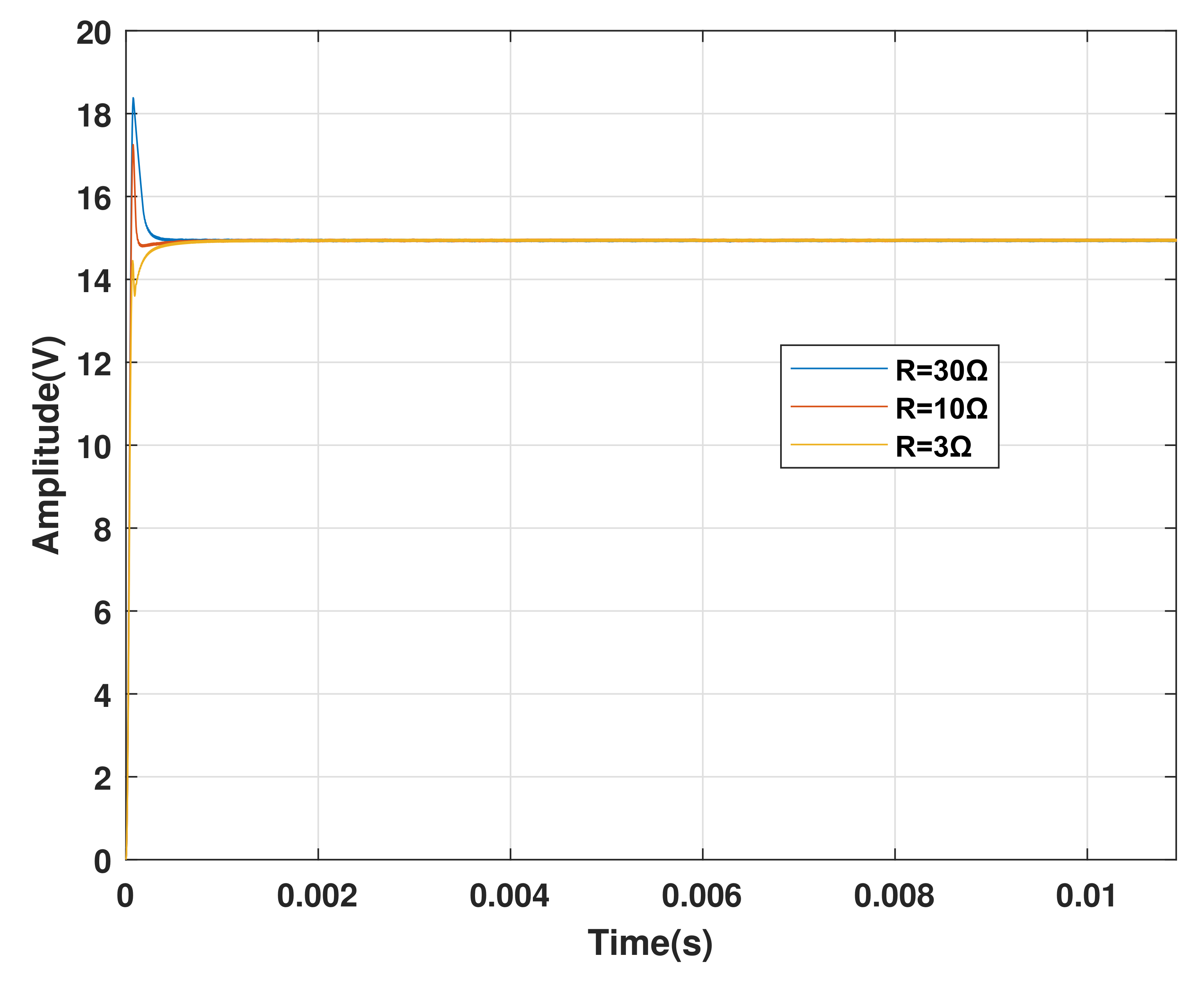
4.3. Response of CI-Optimized System to Parametric Variations
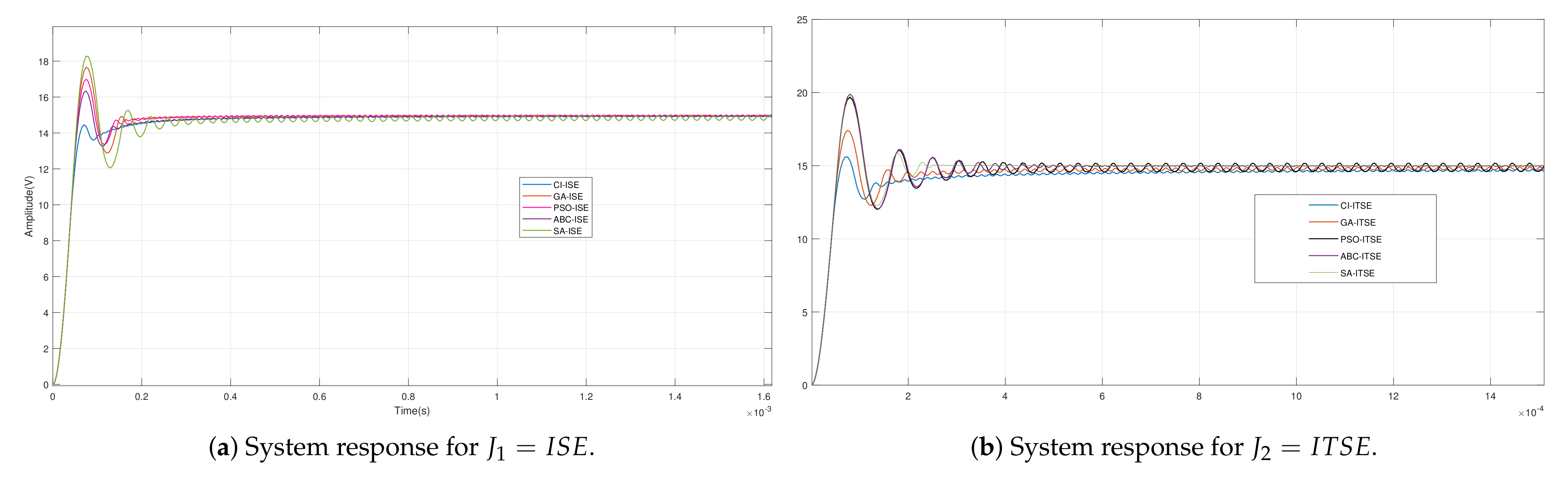
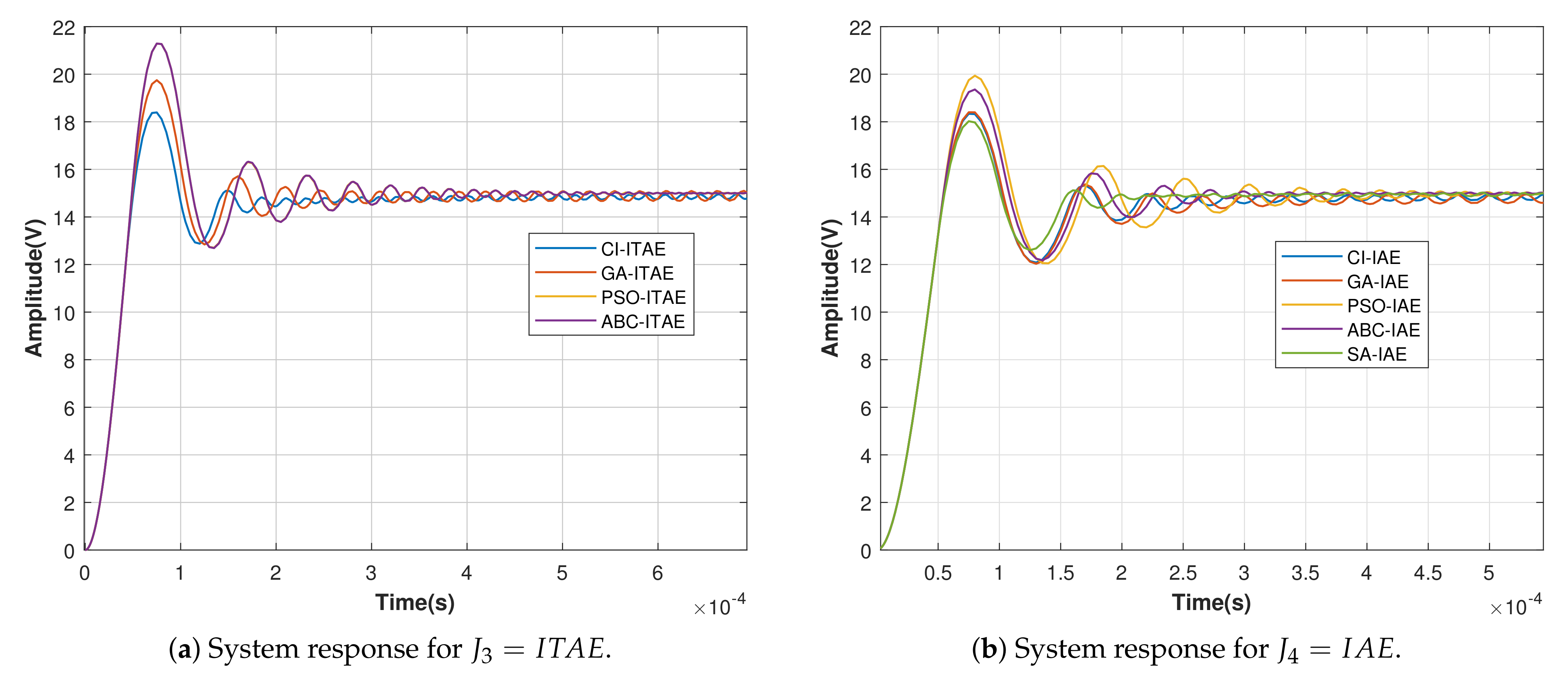
4.4. Performance Comparison of CI
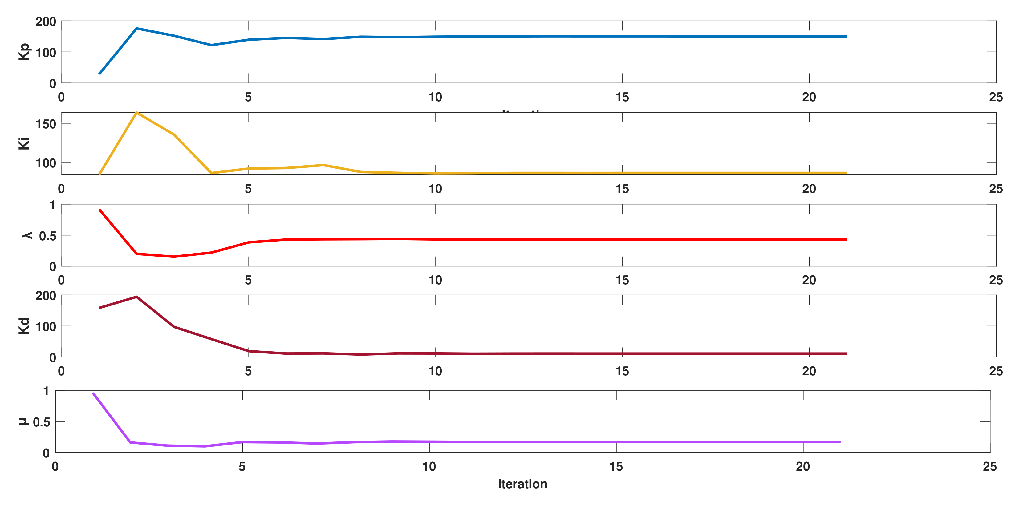
4.5. Convergence Plots of the CI Algorithm
5. Conclusions
Author Contributions
Funding
Institutional Review Board Statement
Informed Consent Statement
Data Availability Statement
Conflicts of Interest
References
- Raviraj, V.S.C.; Sen, P.C. Comparative study of proportional-integral, sliding mode, and fuzzy logic controllers for power converters. IEEE Trans. Ind. Appl. 1997, 33, 518–524. [Google Scholar] [CrossRef] [Green Version]
- Seo, S.W.; Choi, H.H. Digital Implementation of Fractional Order PID-Type Controller for Boost DC–DC Converter. IEEE Access 2019, 7, 142652–142662. [Google Scholar] [CrossRef]
- Habetler, T.G.; Harley, R.G. Power electronic converter and system control. Proc. IEEE 2001, 89, 913–925. [Google Scholar] [CrossRef]
- Vidal-Idiarte, E.; Martinez-Salamero, L.; Guinjoan, F.; Calvente, J.; Gomariz, S. Sliding and fuzzy control of a boost converter using an 8-bit microcontroller. IEE Proc. Electr. Power Appl. 2004, 151, 5–11. [Google Scholar] [CrossRef]
- Chan, H.; Chau, K.T.; Chan, C.C. A neural network controller for switching power converters. In Proceedings of the IEEE Power Electronics Specialist Conference—PESC 93, Seattle, WA, USA, 20–24 June 1993; pp. 887–892. [Google Scholar] [CrossRef]
- Zhang, G.; Li, Z.; Zhang, B.; Halang, W.A. Power electronics converters: Past, present and future. Renew. Sustain. Energy Rev. 2018, 81, 2028–2044. [Google Scholar] [CrossRef]
- Borase, R.; Maghade, D.; Sondkar, S.; Pawar, S. A review of PID control, tuning methods and applications. Int. J. Dyn. Control 2021, 9, 818–827. [Google Scholar] [CrossRef]
- Aström, K.J.; Hägglund, T. PID Controllers—Theory, Design, and Tuning; International Society of Automation (ISA): Pittsburgh, PA, USA, 1995. [Google Scholar]
- Ghosh, A.; Prakash, M.; Pradhan, S.; Banerjee, S. A comparison among PID, Sliding Mode and internal model control for a buck converter. In Proceedings of the IECON 2014—40th Annual Conference of the IEEE Industrial Electronics Society, Dallas, TX, USA, 29 October–1 November 2014; pp. 1001–1006. [Google Scholar] [CrossRef]
- Monje, C.A.; Vinagre, B.M.; Feliu, V.; Chen, Y. Tuning and auto-tuning of fractional order controllers for industry applications. Control Eng. Pract. 2008, 16, 798–812. [Google Scholar] [CrossRef] [Green Version]
- Oustaloup, A.; Levron, F.; Mathieu, B.; Nanot, F.M. Frequency-band complex noninteger differentiator: Characterization and synthesis. IEEE Trans. Circuits Syst. Fundam. Theory Appl. 2000, 47, 25–39. [Google Scholar] [CrossRef]
- Chen, Y.; Petras, I.; Xue, D. Fractional order control—A tutorial. In Proceedings of the 2009 American Control Conference, St. Louis, MI, USA, 10–12 June 2009; pp. 1397–1411. [Google Scholar] [CrossRef]
- Tepljakov, A.; Alagoz, B.B.; Yeroglu, C.; Gonzalez, E.; HosseinNia, S.H.; Petlenkov, E. FOPID Controllers and Their Industrial Applications: A Survey of Recent Results. IFAC-PapersOnLine 2018, 51, 25–30. [Google Scholar] [CrossRef]
- Shah, P.; Agashe, S. Review of fractional PID controller. Mechatronics 2016, 38, 29–41. [Google Scholar] [CrossRef]
- Monje, C.; Chen, Y.; Vinagre, B.; Xue, D.; Feliu, V. Fractional Order Systems and Control—Fundamentals and Applications; Springer: London, UK, 2010. [Google Scholar] [CrossRef]
- Calderón, A.; Vinagre, B.; Feliu, V. Fractional order control strategies for power electronic buck converters. Signal Process. 2006, 86, 2803–2819. [Google Scholar] [CrossRef]
- Tepljakov, A.; Alagoz, B.B.; Yeroglu, C.; Gonzalez, E.A.; Hosseinnia, S.H.; Petlenkov, E.; Ates, A.; Cech, M. Towards Industrialization of FOPID Controllers: A Survey on Milestones of Fractional-Order Control and Pathways for Future Developments. IEEE Access 2021, 9, 21016–21042. [Google Scholar] [CrossRef]
- Prajapati, S.; Garg, M.M.; Prithvi, B. Design of Fractional-Order PI controller for DC-DC Power Converters. In Proceedings of the 2018 8th IEEE India International Conference on Power Electronics (IICPE), Jaipur, India, 13–15 December 2018; pp. 1–6. [Google Scholar]
- Djebbri, S.; Ladaci, S.; Metatla, A. Fractional-order model reference adaptive control of a multi-source renewable energy system with coupled DC/DC converters power compensation. Energy Syst. 2020, 11, 315–355. [Google Scholar] [CrossRef]
- Qi, Z.; Tang, J.; Pei, J.; Shan, L. Fractional Controller Design of a DC-DC Converter for PEMFC. IEEE Access 2020, 8, 120134–120144. [Google Scholar] [CrossRef]
- Sánchez, A.G.S.; Soto-Vega, J.; Tlelo-Cuautle, E.; Rodríguez-Licea, M.A. Fractional-Order Approximation of PID Controller for Buck–Boost Converters. Micromachines 2021, 12, 591. [Google Scholar] [CrossRef] [PubMed]
- Warrier, P.; Shah, P. Fractional Order Control of Power Electronic Converters in Industrial Drives and Renewable Energy Systems: A Review. IEEE Access 2021, 9, 58982–59009. [Google Scholar] [CrossRef]
- Rao, S. Engineering Optimization: Theory and Practice, 4th ed.; John Wiley and Sons: Hoboken, NJ, USA, 2009. [Google Scholar] [CrossRef]
- Karaboga, D.; Gorkemli, B.; Ozturk, C.; Karaboga, N. A comprehensive survey: Artificial bee colony (ABC) algorithm and applications. Artif. Intell. Rev. 2014, 42, 21–57. [Google Scholar] [CrossRef]
- Maiti, D.; Acharya, A.; Chakraborty, M.; Konar, A.; Janarthanan, R. Tuning PID and PIλDσ Controllers using the Integral Time Absolute Error Criterion. In Proceedings of the 2008 4th International Conference on Information and Automation for Sustainability, Colombo, Sri Lanka, 12–14 December 2008. [Google Scholar] [CrossRef]
- Cao, J.-Y.; Liang, J.; Cao, B.-G. Optimization of fractional order PID controllers based on genetic algorithms. In Proceedings of the 2005 International Conference on Machine Learning and Cybernetics, Guangzhou, China, 18–21 August 2005; Volume 9, pp. 5686–5689. [Google Scholar] [CrossRef]
- Das, S.; Pan, I.; Das, S.; Gupta, A. A Novel Fractional Order Fuzzy PID Controller and Its Optimal Time Domain Tuning Based on Integral Performance Indices. Eng. Appl. AI 2012, 25, 430–442. [Google Scholar] [CrossRef] [Green Version]
- Khubalkar, S.; Junghare, A.S.; Aware, M.V.; Chopade, A.; Das, S. Demonstrative fractional order PID controller based DC motor drive on digital platform. ISA Trans. 2017, 82, 79–93. [Google Scholar] [CrossRef] [PubMed]
- Khubalkar, S.; Chopade, A.; Junghare, A.; Aware, M.; Das, S. Design and Realization of Stand-Alone Digital Fractional Order PID Controller for Buck Converter Fed DC Motor. Circuits Syst. Signal Process. 2016, 35, 2189–2211. [Google Scholar] [CrossRef]
- Merrikh-Bayat, F.; Jamshidi, A. Comparing the Performance of Optimal PID and Optimal Fractional-Order PID Controllers Applied to the Nonlinear Boost Converter. arXiv 2013, arXiv:1312.7517. [Google Scholar]
- Amirahmadi, A.; Rafiei, M.; Tehrani, K.; Griva, G.; Bartarseh, I. Optimum Design of Integer and Fractional-Order PID Controllers for Boost Converter Using SPEA Look-up Tables. J. Power Electron. 2015, 15, 160–176. [Google Scholar] [CrossRef] [Green Version]
- Kulkarni, A.J.; Durugkar, I.P.; Kumar, M. Cohort Intelligence: A Self Supervised Learning Behavior. In Proceedings of the Proceedings of the 2013 IEEE International Conference on Systems, Man, and Cybernetics, Manchester, UK, 13–16 October 2013; IEEE Computer Society: Washington, DC, USA, 2013; pp. 1396–1400. [Google Scholar] [CrossRef]
- Kulkarni, A.J.; Baki, M.; Chaouch, B.A. Application of the cohort-intelligence optimization method to three selected combinatorial optimization problems. Eur. J. Oper. Res. 2016, 250, 427–447. [Google Scholar] [CrossRef]
- Kulkarni, A.J.; Shabir, H. Solving 0–1 Knapsack Problem using Cohort Intelligence Algorithm. Int. J. Mach. Learn. Cybern. 2016, 7, 427–441. [Google Scholar] [CrossRef]
- Kulkarni, O.; Kulkarni, N.; Kulkarni, A.; Kakandikar, G. Constrained Cohort Intelligence using Static and Dynamic Penalty Function Approach for Mechanical Components Design. Int. J. Parallel Emergent Distrib. Syst. 2016, 33, 570–588. [Google Scholar] [CrossRef] [Green Version]
- Bhambhani, A.; Shah, P. PID parameter optimization using Cohort intelligence technique for D.C motor control system. In Proceedings of the 2016 International Conference on Automatic Control and Dynamic Optimization Techniques (ICACDOT), Pune, India, 9–10 September 2016; pp. 465–468. [Google Scholar] [CrossRef]
- Rashid, M. Power Electronics: Circuits, Devices, and Applications; Pearson: London, UK, 2009. [Google Scholar]
- AND9135/D LC Selection Guide for the DC-DC Synchronous Buck Converter. ON Semiconductor. 2013. Available online: https://www.onsemi.com/pub/Collateral/AND9135-D.PDF (accessed on 4 August 2021).
- Ejury, J. Buck Converter Design. Infineon Technologies North America. 2013. Available online: https://www.mouser.de/pdfdocs/BuckConverterDesignNote.pdf (accessed on 4 August 2021).
- Caponetto, R.; Dongola, G.; Fortuna, L.; Petráš, I. Fractional Order Systems; World Scientific: Singapore, 2010. [Google Scholar] [CrossRef]
- Loverro, A. Fractional Calculus: History, Definitions and Applications for the Engineer; Univiersity of Notre Dame: Notre Dame, IN, USA, 2004. [Google Scholar]
- Miller, K.; Ross, B. An Introduction to the Fractional Calculus and Fractional Differential Equations; John Wiley and Sons, Inc.: Reading, MA, USA, 1993. [Google Scholar]
- Vinagre, B.; Podlubny, I.; Hernández, A.; Feliu, V. Some approximations of fractional order operators used in control theory. Fract. Calc. Appl. Anal. 2000, 3, 231–248. [Google Scholar]
- Valério, D.; da Costa, J. An Introduction to Fractional Control; The Institution of Engineering and Technology: London, UK, 2012; pp. 1–358. [Google Scholar] [CrossRef]
- Visioli, A. Research trends for PID controllers. Acta Polytech. 2012, 52, 144–150. [Google Scholar] [CrossRef]
- Faieghi, M.; Nemati, A. On Fractional-Order PID Design. In Applications of MATLAB in Science and Engineering; IntechOpen: London, UK, 2011. [Google Scholar] [CrossRef] [Green Version]
- Kulkarni, A.J.; Krishnasamy, G.; Abraham, A. Cohort Intelligence: A Socio-Inspired Optimization Method; Springer: Berlin/Heidelberg, Germany, 2017. [Google Scholar] [CrossRef]
- Patankar, N.S.; Kulkarni, A.J. Variations of Cohort Intelligence. Soft Comput. 2018, 22, 1731–1747. [Google Scholar] [CrossRef]
- Tavazoei, M.S. Notes on integral performance indices in fractional-order control systems. J. Process. Control 2010, 20, 285–291. [Google Scholar] [CrossRef]
- Duarte-Mermoud, M.; Prieto, R. Performance index for quality response of dynamical systems. ISA Trans. 2004, 43, 133–151. [Google Scholar] [CrossRef] [Green Version]
- Richard, C.; Bishop, R.H. Modern Control Systems; Pearson Prentice Hall, Inc.: Upper Saddle River, NJ, USA, 2008. [Google Scholar]
- Shah, P.; Agashe, S.; Kulkarni, A. Design of fractional PID controller using the cohort intelligence method. Front. Inf. Technol. Electron. Eng. 2017, 19, 437–445. [Google Scholar] [CrossRef]
- Fraga-Gonzalez, L.; Fuentes, R.; García-González, A.; Sanchez-Ante, G. Adaptive simulated annealing for tuning PID controllers. AI Commun. 2017, 30, 347–362. [Google Scholar] [CrossRef]
- GirirajKumar, S.M.; Bodla, R.; Narayanan, A. Design of Controller using Simulated Annealing for a Real Time Process. Int. J. Comput. Appl. 2010, 6, 20–25. [Google Scholar] [CrossRef]


| Parameter | Value |
|---|---|
| Filter Inductance | 70 H |
| Filter Capacitance | 22 F |
| Load resistance, R | 3 |
| Switching frequency | 100 KHz |
| Input voltage | 24 V |
| Output voltage | 15 V |
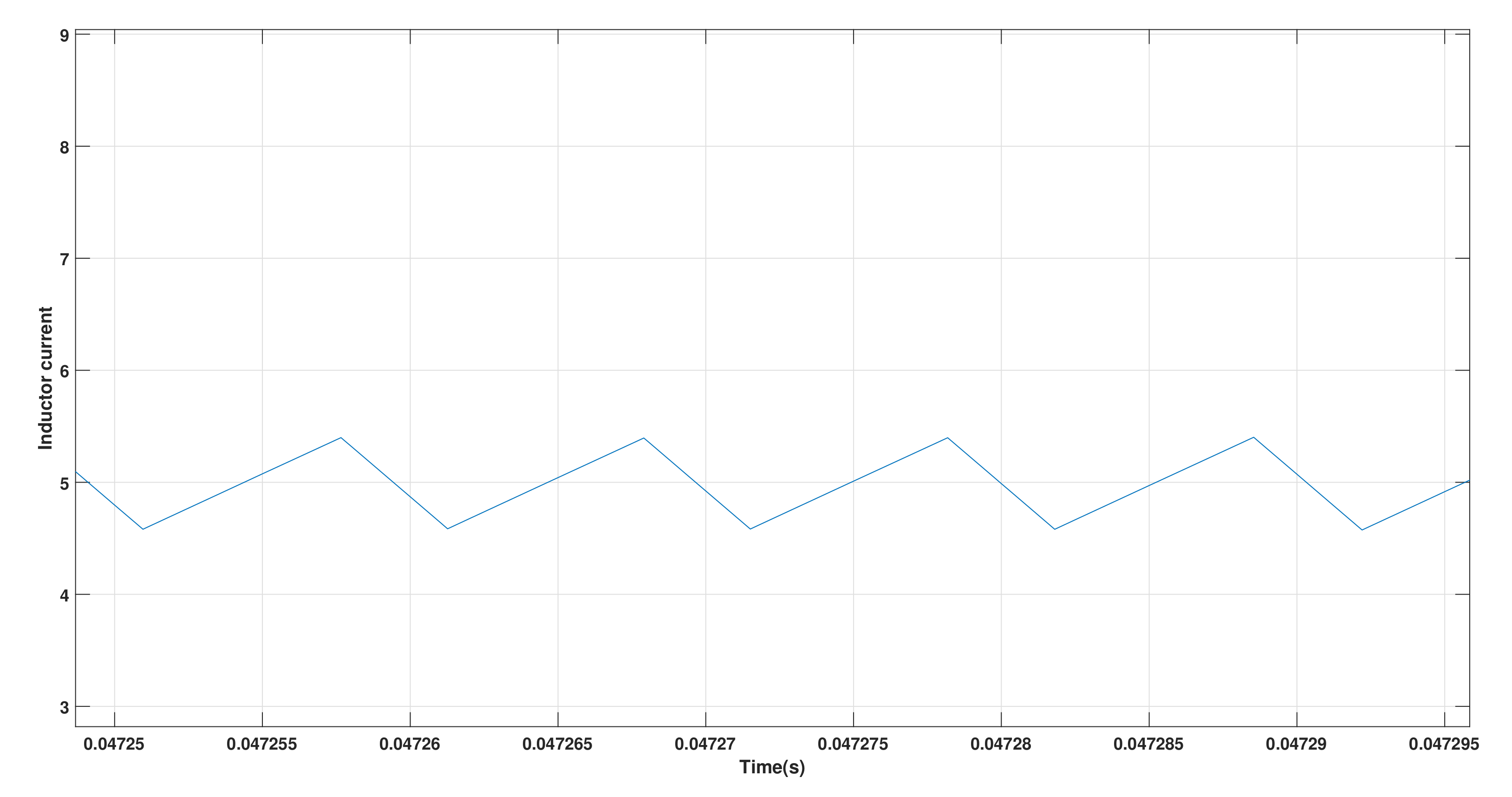
| Inductor current ripple | 20% of |
| Parameters | Values |
|---|---|
| No. of cohort candidates | 4–5 |
| No. of variables | 5 |
| Reduction factor | 0.45, 0.55 |
| Convergence constant | 0.001 |
| Maximum iterations | 25 |
| Parameters | ISE ( = 0.45) | ITSE ( = 0.55) | ITAE ( = 0.45) | IAE ( = 0.45) |
|---|---|---|---|---|
| 162.08 | 27.9709 | 123.0768 | 197.3838 | |
| 133.84 | 112.7302 | 122.9522 | 115.0357 | |
| 0.5851 | 0.7737 | 54.0215 | 63.0392 | |
| 0.0673 | 0.1022 | 0.4738 | 0.3730 | |
| 0.6107 | 0.5868 | 0.2537 | 0.1874 | |
| Mp (%) | 0 | 0 | 20 | 21.3 |
| Tr (ms) | 0.037 | 0.035 | 0.0365 | 0.0354 |
| Tss (ms) | 0.265 | 0.35 | 0.27 | 0.3 |
| Cost function value | 0.006 | 0.0288 | 0.0004 | 0.0119 |
| Parameters | |||||
|---|---|---|---|---|---|
| CI | GA | PSO | ABC | SA | |
| Avg. Overshoot % | 5.6 | 14.6 | 16.2 | 18 | 21 |
| Rise Time (ms) | 0.037 | 0.038 | 0.036 | 0.035 | 0.035 |
| Settling time (ms) | 0.265 | 0.19 | 0.167 | 0.24 | 0.32 |
| Cost function | 0.006 | 0.0057 | 0.0063 | 0.0067 | 0.0064 |
| Avg. computation Time (s) | 542 | 1600 | 720 | 1100 | 1800 |
| Avg. Function evaluations | 84 | 242 | 88 | 100 | 400 |
| Avg. No. of iterations | 21 | 60 | 22 | 25 | 100 |
| Parameters | |||||
|---|---|---|---|---|---|
| CI | GA | PSO | ABC | SA | |
| Avg. Overshoot % | 9.2 | 16.11 | 5 | 17.3 | 25 |
| Rise Time (ms) | 0.042 | 0.038 | 0.043 | 0.039 | 0.039 |
| Settling time (ms) | 0.39 | 0.42 | 0.37 | 0.38 | 0.27 |
| Cost function value | 0.0001 | 0.00018 | 1.7 × 10 | 1.7 × 10 | 0.00039 |
| Avg. computation Time (s) | 762 | 1500 | 1200 | 1500 | 1320 |
| Avg. Function evaluations | 84 | 204 | 88 | 100 | 1000 |
| Avg. No. of iterations | 21 | 51 | 21 | 25 | 200 |
| Parameters | |||||
|---|---|---|---|---|---|
| CI | GA | PSO | ABC | SA | |
| Avg. Overshoot % | 20 | 29 | 26 | 18 | - |
| Rise Time (ms) | 0.036 | 0.037 | 0.039 | 0.036 | - |
| Settling time (ms) | 0.31 | 0.36 | 0.39 | 0.40 | - |
| Cost function value | 4 × 10 | 3.44 × 10 | 3.97 × 10 | 2.65 × 10 | 3.97 × 10 |
| Avg. computation Time (s) | 1020 | 1500 | 1200 | 1500 | 1800 |
| Avg. Function evaluations | 84 | 204 | 88 | 100 | 1000 |
| Avg. No. of iterations | 21 | 51 | 21 | 25 | 200 |
| Parameters | |||||
|---|---|---|---|---|---|
| CI | GA | PSO | ABC | SA | |
| Avg. Overshoot % | 20 | 21 | 25 | 18 | 25 |
| Rise Time (ms) | 0.036 | 0.038 | 0.039 | 0.036 | 0.037 |
| Settling time (ms) | 0.28 | 0.42 | 0.39 | 0.38 | 0.29 |
| Cost function value | 0.0116 | 0.00548 | 0.0017 | 0.0024 | 0.005 |
| Avg. computation Time (s) | 542 | 1500 | 1200 | 1500 | 1320 |
| Avg. Function evaluations | 84 | 204 | 88 | 100 | 1000 |
| Avg. No. of iterations | 21 | 51 | 21 | 25 | 200 |
Publisher’s Note: MDPI stays neutral with regard to jurisdictional claims in published maps and institutional affiliations. |
© 2021 by the authors. Licensee MDPI, Basel, Switzerland. This article is an open access article distributed under the terms and conditions of the Creative Commons Attribution (CC BY) license (https://creativecommons.org/licenses/by/4.0/).
Share and Cite
Warrier, P.; Shah, P. Optimal Fractional PID Controller for Buck Converter Using Cohort Intelligent Algorithm. Appl. Syst. Innov. 2021, 4, 50. https://doi.org/10.3390/asi4030050
Warrier P, Shah P. Optimal Fractional PID Controller for Buck Converter Using Cohort Intelligent Algorithm. Applied System Innovation. 2021; 4(3):50. https://doi.org/10.3390/asi4030050
Chicago/Turabian StyleWarrier, Preeti, and Pritesh Shah. 2021. "Optimal Fractional PID Controller for Buck Converter Using Cohort Intelligent Algorithm" Applied System Innovation 4, no. 3: 50. https://doi.org/10.3390/asi4030050
APA StyleWarrier, P., & Shah, P. (2021). Optimal Fractional PID Controller for Buck Converter Using Cohort Intelligent Algorithm. Applied System Innovation, 4(3), 50. https://doi.org/10.3390/asi4030050