Classification of Alzheimer’s Disease Patients Using Texture Analysis and Machine Learning

Abstract

Alzheimer’s disease (AD) has been studied extensively to understand the nature of this complex disease and address the many research gaps concerning prognosis and diagnosis. Several studies based on structural and textural characteristics have already been conducted to aid in identifying AD patients. In this work, an image processing methodology was used to extract textural information and classify the patients into two groups: AD and Cognitively Normal (CN). The Gray Level Co-occurrence Matrix (GLCM) was employed since it is a strong foundation for texture classification. Various textural parameters derived from the GLCM aided in deciphering the characteristics of a Magnetic Resonance Imaging (MRI) region of interest (ROI). Several commonly used image classification algorithms were employed. MATLAB was used to successfully derive 20 features based on the GLCM of the MRI dataset. Based on the data analysis, 8 of the 20 features were determined as significant elements. Ensemble (90.2%), Decision Trees (88.5%), and Support Vector Machine (SVM) (87.2%) were the best performing classifiers. It was observed in GLCM that as the distance (d) between pixels increased, the classification accuracy decreased. The best result was observed for GLCM with d = 1 and direction (d, d, −d) with age and structural data.

1. Introduction

Alzheimer’s Disease (AD) has been extensively studied to better understand this complex disease’s nature and address the numerous unresolved challenges concerning prognosis and diagnosis. According to current projections, the number of people with dementia globally will rise to 75 million by 2030, up from 47 million in 2020.

The hippocampus is vital in developing, structuring, and storing new memories and the association of sensations and feelings with some of these memories. AD causes gradual tissue loss throughout the brain. Hippocampal atrophy is a significant biomarker used to assess and detect AD. The hippocampus undergoes multiple small-scale alterations before a significant change occurs. These changes are visible in clinical magnetic resonance imaging (MRI) at the current resolution. Previous research has demonstrated that texture-based classification produces better results than volume-based classification [1]. The hippocampus appears to demonstrate the most rapid loss of tissue early in the disease course. The increasing atrophy of the hippocampus is responsible for Alzheimer’s-related short-term memory loss [2].

MRI is a highly effective technology for nonaggressive in vivo imaging of the human brain. A widely proven approach is used for robust cross-sectional and longitudinal segmentation of Alzheimer’s Disease Neuroimaging.

Initiative Alzheimer’s Disease Neuroimaging Initiative (ADNI) cohort brain MRI. Structural Magnetic Resonance Imaging (sMRI) detects subtle anatomical changes in the brain to detect AD [3]. MRI is favoured over other modalities for detecting structural changes in the brain caused by neurodegenerative diseases and its significance in AD diagnosis and prognosis [4]. In most sMRI investigations, large-scale tissue changes have been used as biomarkers based on derived features like atrophy to acquire a better diagnosis of AD. Subtle neurodegenerative changes can be noticed and analyzed using statistical properties acquired from texture analysis on an MRI based on a biomarker.

Medical imaging is obtaining images of body parts for diagnostic applications such as detecting or studying diseases. Every week, millions of imaging tasks are performed around the world. Medical imaging is quickly evolving because of advances in image processing methods such as image recognition, analysis, and enhancement. Image processing improves the proportion and quantity of recognized tissues.

Machine learning is a pattern recognition technique that can be used in medical imaging. It is a vital tool that can aid in medical diagnosis. Typically, machine learning begins with the machine learning algorithm system determining the image attributes that are thought to be important in producing the desired prediction or diagnosis. The machine learning algorithm system then determines the optimum solution of these image attributes for classification.

The contributions of this research work are:

• To use texture analysis to examine the minor changes in the hippocampus caused by AD.
• To extract features by implementing texture analysis technique on MRI.
• To classify subjects into AD and cognitively normal (CN) groups by providing the information extracted as input for training machine learning models.

An extensive literature survey was performed, which helped delimit the research domain, and focus is directed to the crucial issues to be resolved. Gray Level Co-occurrence Matrix (GLCM) has been verified to be a standard statistical process of extricating textural characteristics from illustrations. The number of grey levels in the image are equivalent to the rows and columns of a GLCM. GLCM was used to acquire textural features. Angular Second Moment (ASM), Inverse Difference Moment, Entropy and Correlation were the second-order features calculated using the GLCM. High discrimination accuracy was achieved by offering these features for image approximation [5]. Xia, H. et al., considered the bilateral hippocampus and medial temporal lobe (MTL) for volumes and texture features in AD subject’s MRI. Texture features were extracted using GLCM on 66 subjects; 29 of these were AD subjects. Texture features and corresponding volumes were analyzed for correlation between them. Volumes and texture features between the AD and CN group in both the hippocampus and MTL were found to be significantly different. The texture features matching to volumes of both positions were correlated. The CN group was further classified into the non-demented (EC) and young control (YC) group. Texture analysis and volumetry may aid in AD diagnosis, indicating no significant difference in CN groups. It implies that atrophy is observed to be distinct in AD and be an age and AD-associated change [6].

Mohanaiah, P. et al., describes how to use the GLCM to extract texture features for image motion approximation. The Xilinx FPGA was used to compute the four features: ASM, Correlation, Entropy, and Inverse Difference Moment. The findings confirm that the texture features have excellent discriminating precision, take minimal calculation time, and can thus be employed effectively for real-time pattern recognition applications [7]. Fuse, H. et al. investigated the efficacy of classifying CN and AD patients relying on brain texture features. As for shape features, a P-type Fourier descriptor was used, and the lateral ventricle except for the septum lucidum was studied. They had used SVM to conduct classification utilizing a collection of multiple characteristics as features. The classifier accuracy was 87.5%, which was higher than the accuracy reached using volume ratio to intracranial volume (81.5%), which is frequently recognized for traditional evaluation of degenerative characteristics. As per recent research, shape information may be more relevant in diagnosis than traditional volume ratio [1]. Telagarapu P. et al. examined AD in T1-weighted MRI combining Texture Features and the k-NN Classifier. Texture features were obtained via GLCM. With the sole purpose of evaluating the suggested approach, tests were undertaken on the MRI obtained from the OASIS dataset. The presented method has a typical testing accuracy of 74.73%, suggesting that it can differentiate AD and CN effectively [3]. Martinez-Murcia et al. intended to better understand the disease’s development by evaluating neuropsychological test results based purely on MRI data. To accomplish this, they used a deep convolutional auto encoder to do a self-supervised segmentation of the MRI data. The dispersion of features in the z-layer was then employed in a neural regression to a complex linear relationship. Then to see if these imaging-derived indicators are associated with various neuropsychological tests. R² rates of more than 0.3 were achieved in predicting neuropsychological analysis results, with correlations greater than 0.5 in the case of variables significantly associated with neurodegeneration and cognitive states, such as the MMSE or the ADASS11 scores [8,9,10].

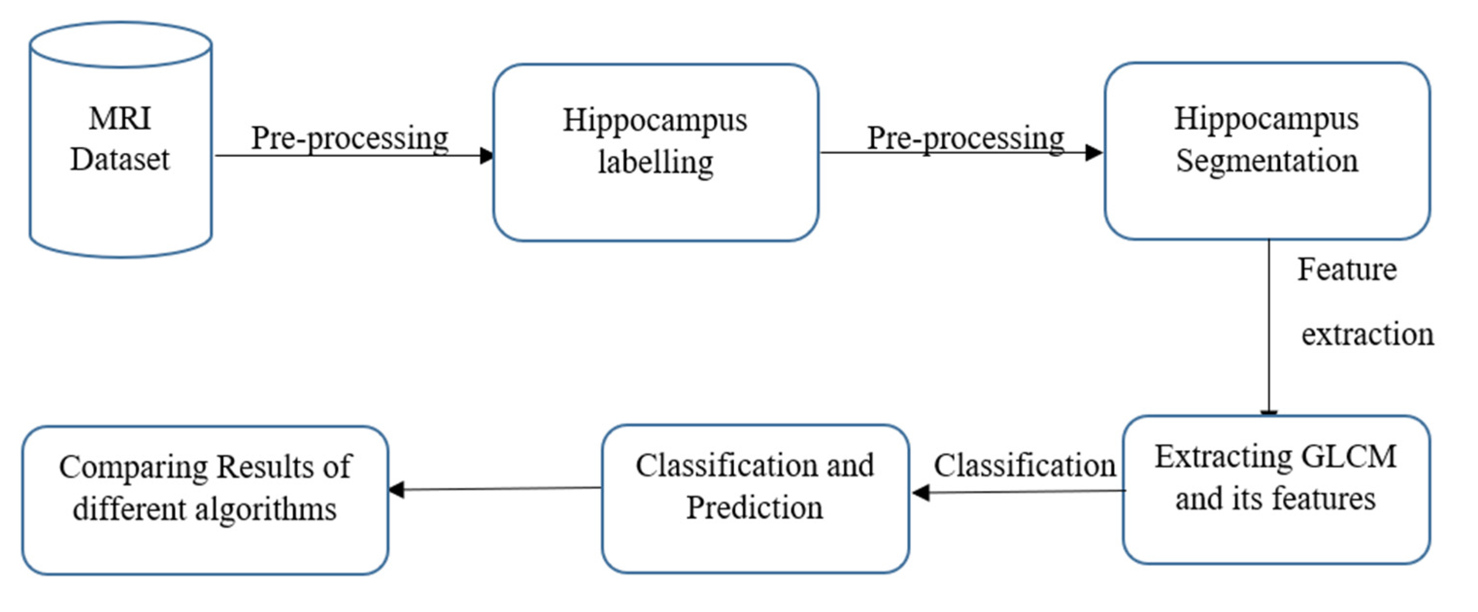
2. Materials and Methods

2.1. Alzheimer’s Disease Neuroimaging Initiative

The ADNI database was used to collect data for this inquiry; as shown in Figure 1, collecting the necessary database was the first stage of this endeavour. ADNI began in 2003 as a public–private partnership directed by lead investigator Michael W. Weiner, MD. The key objective of ADNI would be to see if serial MRI, PET, other biological markers, and clinical and cognitive tests could be used to track the development of early AD. The ADNI research is a multisite longitudinal study aimed at finding clinical, imaging, genetic, and biochemical indicators for initial tracking and AD identification. More than a decade has passed since its beginnings; it has made significant contributions to AD research, enabling researchers worldwide to share data [11].

2.2. MRI Data and Subjects

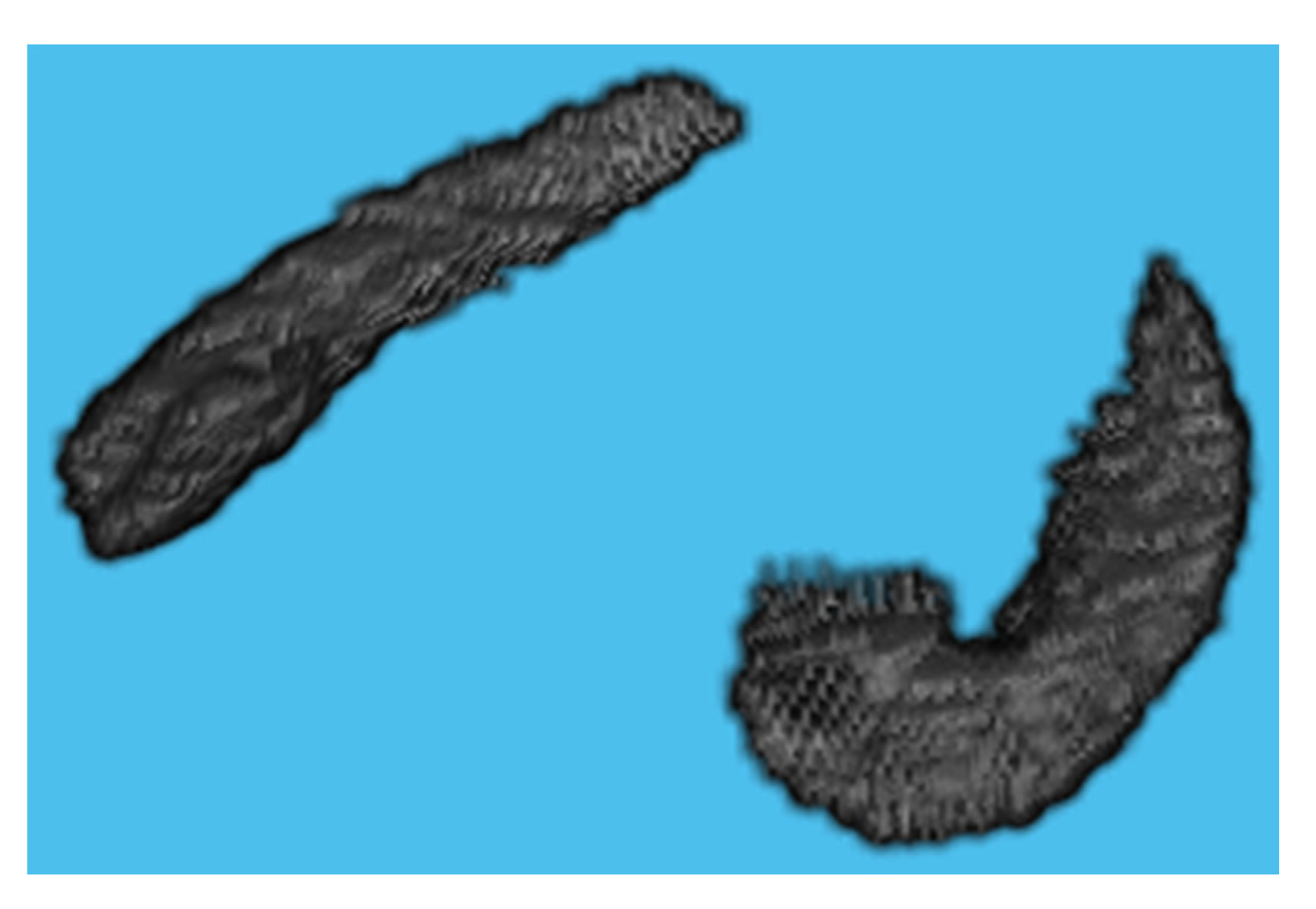
The Image and Data Archive (IDA) search returns raw, unprocessed images based on various selection parameters. Few criteria were used, including a study group in which AD and CN groups were chosen with T1 weighted MRI with slice thickness between 1 mm to 2.5 mm. Three-dimensional Magnetization-prepared Rapid Acquisition Gradient Echo (MPRAGE) MRI with a field strength of 3T is specified for the acquisition. When evaluating texture features extracted from a 1.5T MRI to texture features retrieved from a 3T MRI, it is feasible to identify even more changes in texture characteristics, which could lead to an earlier diagnosis [12,13]. Instead of the original acquisition format (Digital Imaging and Communications in Medicine DICOM), all the MRIs were downloaded in Nifti format [14].

Table 1. Demographical data of the Subjects in detail.

Group	Description	Subject Age
AD	Number of Cases- 119	-
	Minimum	55
	Maximum	91
	Mean (Standard Deviation)	75.10 (±8.60)
CN	Number of Cases- 115	-
	Minimum	59
	Maximum	90
	Mean (Standard Deviation)	74.80 (±7.95)

describes the Demographical data of the subjects in details

The ADNI dataset included MRIs from 234 subjects, with 119 (50.9%) being AD and 115 (49.1%) being CN. The youngest participants were 55 and 59 years old in the AD and CN groups, respectively, while the oldest were 91 and 90.

The dataset was divided into 70% for training and 30% for testing. While training all the all the models, 5-fold cross-validation is used to avoid overfitting. In this technique, the data was split into k = 5 subsets, where one subset is treated as a validation set for the model and k−1, i.e., four subsets for training the model. The data samples were single-trained and then split for validation testing.

2.3. ROI Selection

volBrain is an MRI brain volumetry system available online. volBrain is a fully automated system that can deliver brain structure volumes without the need for human participation. volBrain is mainly composed of image processing tasks that strive to increase the performance of the input images and organize them in a predefined geometric and intensity space so that they may be segmented later [15].

Figure 2 shows the functional block scheme of volBrain. It comprises the HIPS pipeline devised to cope with high-resolution or standard T1w images (Spoiled Gradient Echo (SPGR) and MPRAGE at 1.5T and 3T, respectively) without any preprocessing. T1 weighted sequences are used substantially in all MRI treatments and are best described as the most “anatomical” of images, that closely resemble the looks of tissues macroscopically. HIPS considers the use of the Winterburn segmentation protocol, which is freely available. MOPAL, which performs quick segmentation, offers accurate findings in less than twenty minutes and provides a mask of Winterburn segmentation protocol with reports stating the volumes of all the subfields and the total volume of the structure. HIPS exceeds other state-of-the-art algorithms regarding segmentation accuracy, earning a DICE of 0.661 for the Winterburn dataset. CA1, CA2/CA3, CA4/DG, SR/SL/SM, and Subiculum are the five subfields in the Winterburn dataset, as shown in Figure 3. volBrain is one of the first few freely available platforms that offer hippocampus segmentation based on the European Alzheimer’s Disease Consortium (EADC) protocol, which will become the standard definition for AD in the next few years [15,16]. In terms of volume and shape estimation, volBrain is deemed more reliable than Freesurfer and FIRST [16].

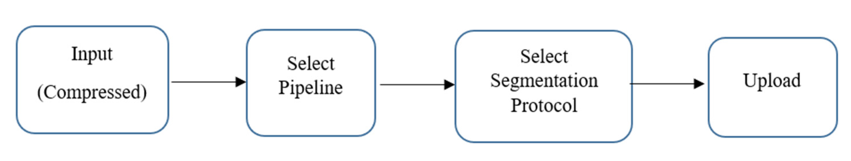
2.4. Hippocampus Segmentation

MRIcron is a cross-platform image viewer for the Nifti format. It can import several layers of images, produce volume renderings, and draw volumes of interest. It also incorporates Node Package Manager (NPM) for statistics and dcm2nii for converting DICOM images to Nifti format. We employed MRIcron to segment the data [17,18]. The complete brain scan is the data set obtained from ADNI. MRI data were processed by this program to obtain the ROI, which yielded only the hippocampus region with its original grey intensities preserved. We overlaid the Winterburn segmentation mask generated by volBrain on the original MRI and maintained the area beneath the mask, removing the pixels beyond the mask boundary as shown in Figure 4.

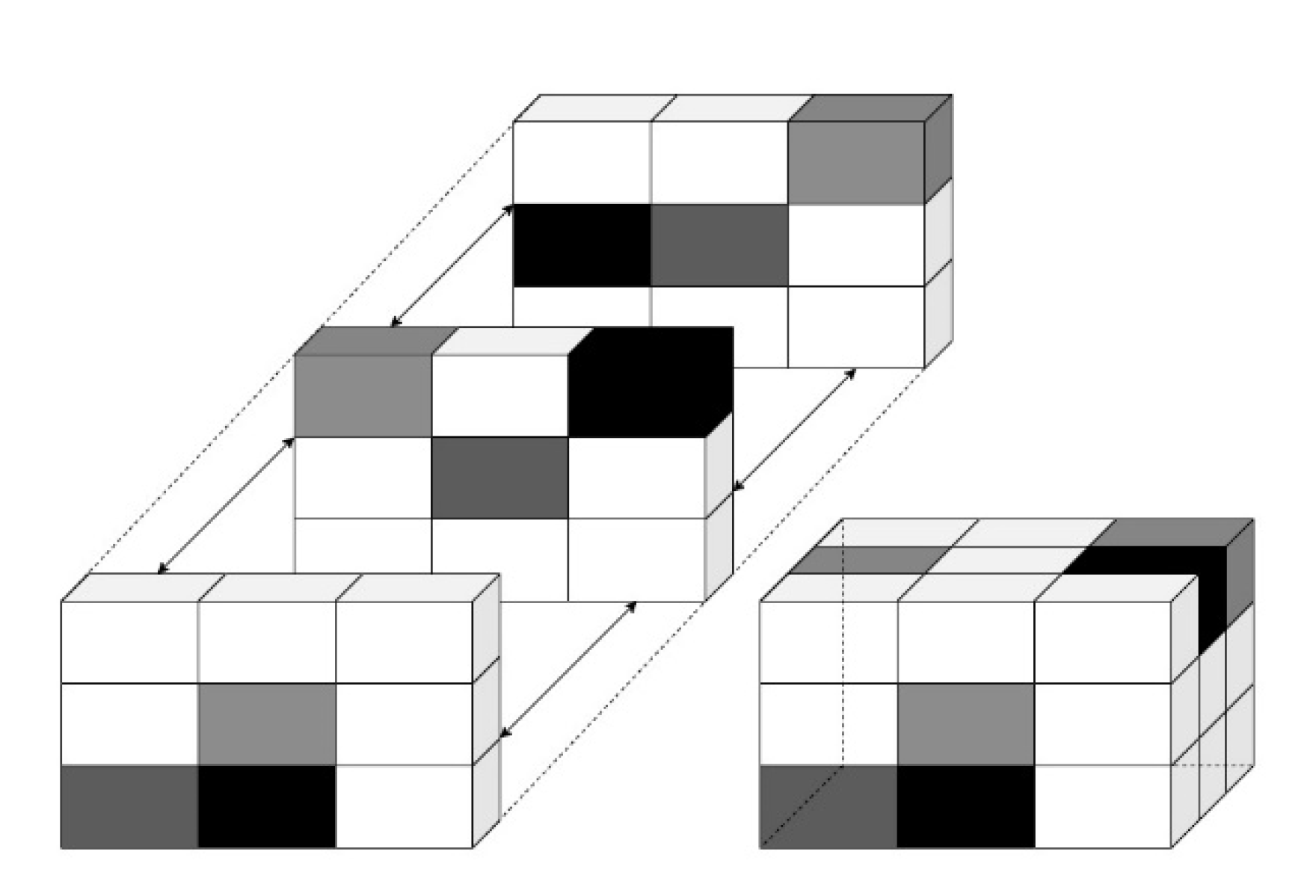
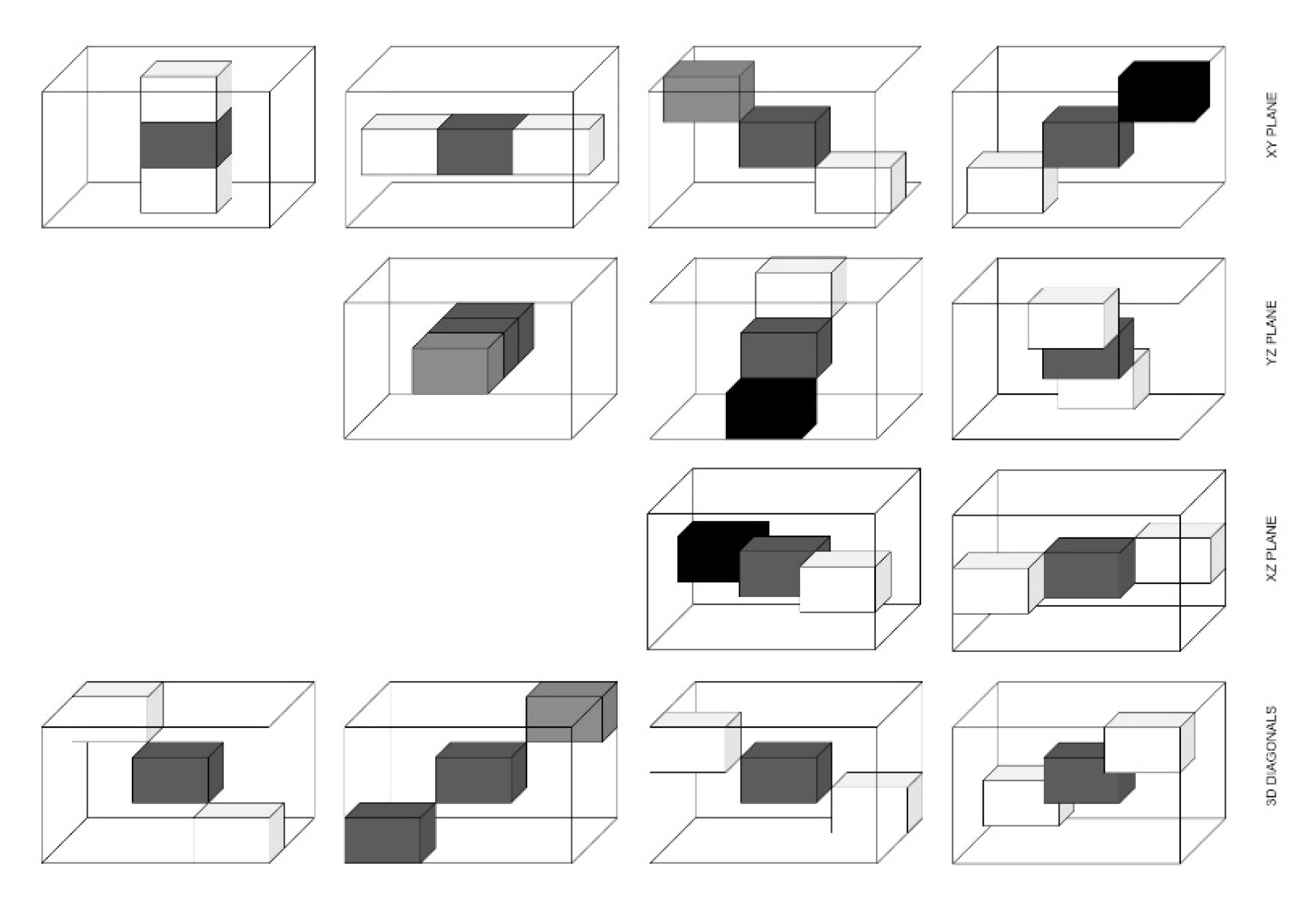
2.5. Texture Analysis

The texture is a crucial feature for recognizing ROI in an image. Haralick et al. [5] introduced GLCM as one of the first methods for texture feature extraction in 1973. For texture analysis, GLCM was used. The two pixels are considered at a time namely the reference and the neighbour pixel. The grey level distribution of pairs of pixels in a specific distance and image configuration was analyzed by GLCM, reflecting the texture or spatial arrangements of pixel intensities existing in ROI. The four directions of two-dimensional (2D) GLCM are 0°, 45°, 90°, and 135°, but for 3D GLCM, there are thirteen independent directions as described in

Table 2. Directions for 3D GLCM.

Sr. No.	Directions
1	(0, 0, d)
2	(0, d, −d)
3	(0, d, 0)
4	(d, 0, −d)
5	(0, d, d)
6	(d, d, −d)
7	(−d, d, −d)
8	(d, 0, 0)
9	(d, 0, d)
10	(d, d, 0)
11	(−d, d, 0)
12	(d, d, d)
13	(−d, d, d)

d = distance between pixels.

.

At short distances d, GLCM provides fine texture, whereas it provides coarse texture in longer distances. The roughness of texture is associated with spatial frequency. Coarse texture has a low spatial frequency, while fine texture has a high spatial frequency. Before computing the GLCM, we defined a certain spatial relationship between the reference and neighbouring pixels, as shown in Figure 5.

The Figure 6 shows distances mentioned in terms of the X, Y and Z-axis [19,20].

A GLCM is generated by size (Range of Intensities x Range of Intensities).

All intensities are initialized to 0 once a spatial relationship is defined. By transversely going through the image. Identifying the defined spatial relationship for every pair of intensities, and incrementing that cell in the matrix. The texture attributes can be calculated from the matrix to represent the textures in the image once the GLCM has been calculated. Haralick retrieved the following features from the GLCMs to characterize texture. A few features are shown in

Table 3. GLCM features and their equations.

Sr. No.	Feature	Formula	Notations
1	Autocorrelation	$f_1={\displaystyle {\displaystyle \sum }_i^{N_g}}{\displaystyle {\displaystyle \sum }_j^{N_g}}ij{M}_{ij}$	$N_g$–number of grey levels. i–row number j–column number
2	Contrast	$f_2={\displaystyle {\displaystyle \sum }_{n=0}^{N_g=1}}{n}^2\left\{{\displaystyle {\displaystyle \sum }_i^{N_g}}{\displaystyle {\displaystyle \sum }_j^{N_g}}{M}_{ij}\right\}$	$M_{ij}$–Element i,j of the normalized symmetrical GLCM $n$–number of paired data
3	Correlation	$f_3={\displaystyle {\displaystyle \sum }_i^{N_g}}{\displaystyle {\displaystyle \sum }_j^{N_g}}\frac{ij{M}_{ij}-{\mu }_x{\mu }_y}{{\sigma }_x{\sigma }_y}$	$\mu$–the GLCM mean (being an estimate of the intensity of all pixels in the relationships that contributed to the GLCM) $\sigma$–the variance of the intensities of all reference pixels in the relationships that contributed to the GLCM (symmetric)
4	Cluster Prominence	$f_4={\displaystyle {\displaystyle \sum }_i^{N_g}}{\displaystyle {\displaystyle \sum }_j^{N_g}}{M}_{ij} {\left(i+j-{\mu }_i-{\mu }_j\right)}^4$
5	Cluster Shade	$f_5={\displaystyle {\displaystyle \sum }_i^{N_g}}{\displaystyle {\displaystyle \sum }_j^{N_g}}{M}_{ij} {\left(i+j-{\mu }_x-{\mu }_y\right)}^3$
6	Dissimilarity	$f_6={\displaystyle {\displaystyle \sum }_i^{N_g}}{\displaystyle {\displaystyle \sum }_j^{N_g}}{M}_{ij} \left|i-j\right|$
7	Energy	$f_7={\displaystyle {\displaystyle \sum }_i^{N_g}}{\displaystyle {\displaystyle \sum }_j^{N_g}}{M}_{ij}{}^2$
8	Entropy	$f_8=-{\displaystyle {\displaystyle \sum }_i^m}{\displaystyle {\displaystyle \sum }_j^n}{M}_{ij} \log \left(M_{ij}\right)$
9	Homogeneity	$f_9={\displaystyle {\displaystyle \sum }_i^{N_g}}{\displaystyle {\displaystyle \sum }_j^{N_g}}\frac{M_{ij}}{1+\left|i-j\right|}$
10	Maximum Probability	$f_{10}=\underset{i,j}{\max }{M}_{ij}$
11	Variance	$f_{11}={\displaystyle {\displaystyle \sum }_i^{N_g}}{\displaystyle {\displaystyle \sum }_j^{N_g}}{\left(i-\mu \right)}^2{M}_{ij}$
12	Sum average	$f_{12}={\displaystyle {\displaystyle \sum }_{n=2}^{N_g}}n{M}_{x+y,n}$
13	Sum variance	$f_{13}={\displaystyle {\displaystyle \sum }_{n=2}^{2N_g}}{\left(n-f_{14}\right)}^2{M}_{x+y,n}$
14	Sum entropy	$f_{14}={\displaystyle {\displaystyle \sum }_{n=2}^{2N_g}}{M}_{x+y,n}\log \left(M_{x+y,n}\right)$
15	Difference variance	$f_{15}=Var\left(M_{x-y}\right)$
16	Difference entropy	$f_{16}={\displaystyle {\displaystyle \sum }_{n=0}^{N_g-1}}{M}_{x-y,n}\log (M_{x-y,n})$
17	Information measure of correlation1	$f_{17}=\frac{f_8-HX{Y}_1}{\max \left\{HX,HY\right\}}$	$HX$ and $HY$ are entropies of $M_x$ and $M_y$
18	Information measure of correlation2	$f_{18}={\left[1-e^{-2\left(HX{Y}_2-f_9\right)}\right]}^{\frac{1}{2}}$
19	Inverse difference	$f_{19}={{\displaystyle \sum }}^{ }\frac{M_{ij}}{1+{\left(i-j\right)}^2}$
20	Inverse difference moment normalized	$f_{20}={\displaystyle {\displaystyle \sum }_i^{N_g}}{\displaystyle {\displaystyle \sum }_j^{N_g}}\frac{M_{ij}}{1+{\left(i-j\right)}^2}$

[5,21,22].

2.6. Classification Models

2.6.1. Support Vector Machine (SVM)

For clean and preprocessed data that is linearly separable, SVM creates a hyperplane between the support vectors called the decision boundary, as shown in Figure 7. Data points on either side of the decision boundary belong to different classes. The hyperplane is one dimension lower than the dimension of the dataset; e.g., if the dataset is three-dimensional, the hyperplane would be two-dimensional. SVM tries to maximize the margin from the closest points of each class using supervised learning [23,24].

2.6.2. Decision Trees

A decision tree is a supervised learning algorithm. It is used when there is a nonlinear or complex nonlinear relationship between independent and dependent variables. First, it divides the dataset into different nodes/leafs, as shown in Figure 8. Then, based on the number of target variables, these nodes are split further into different subnodes; a node that cannot be split into more subnodes is called the terminal node. Based on the dataset, different algorithms can be used for doing the split in the available variables [25].

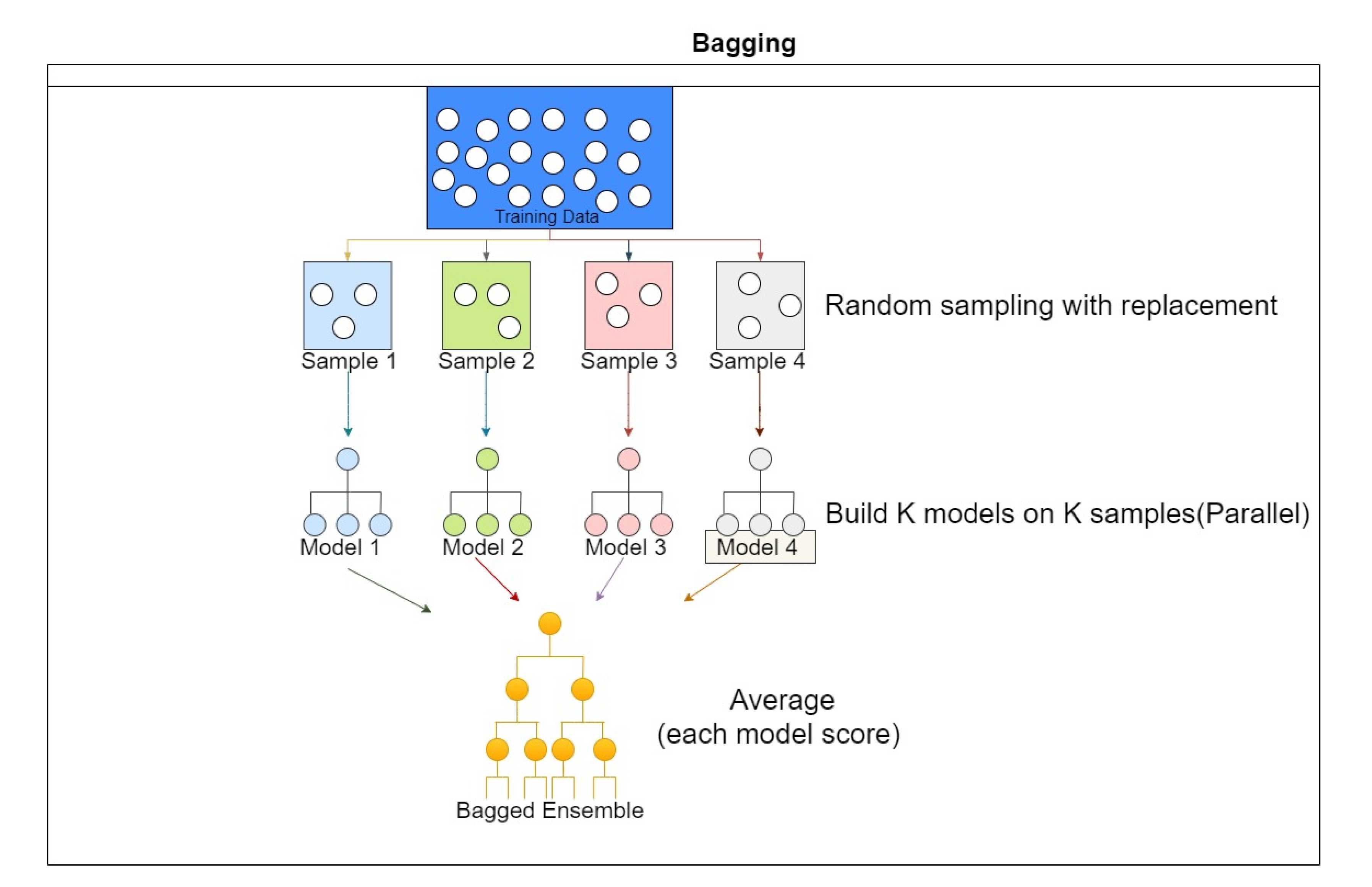
2.6.3. Random Forest

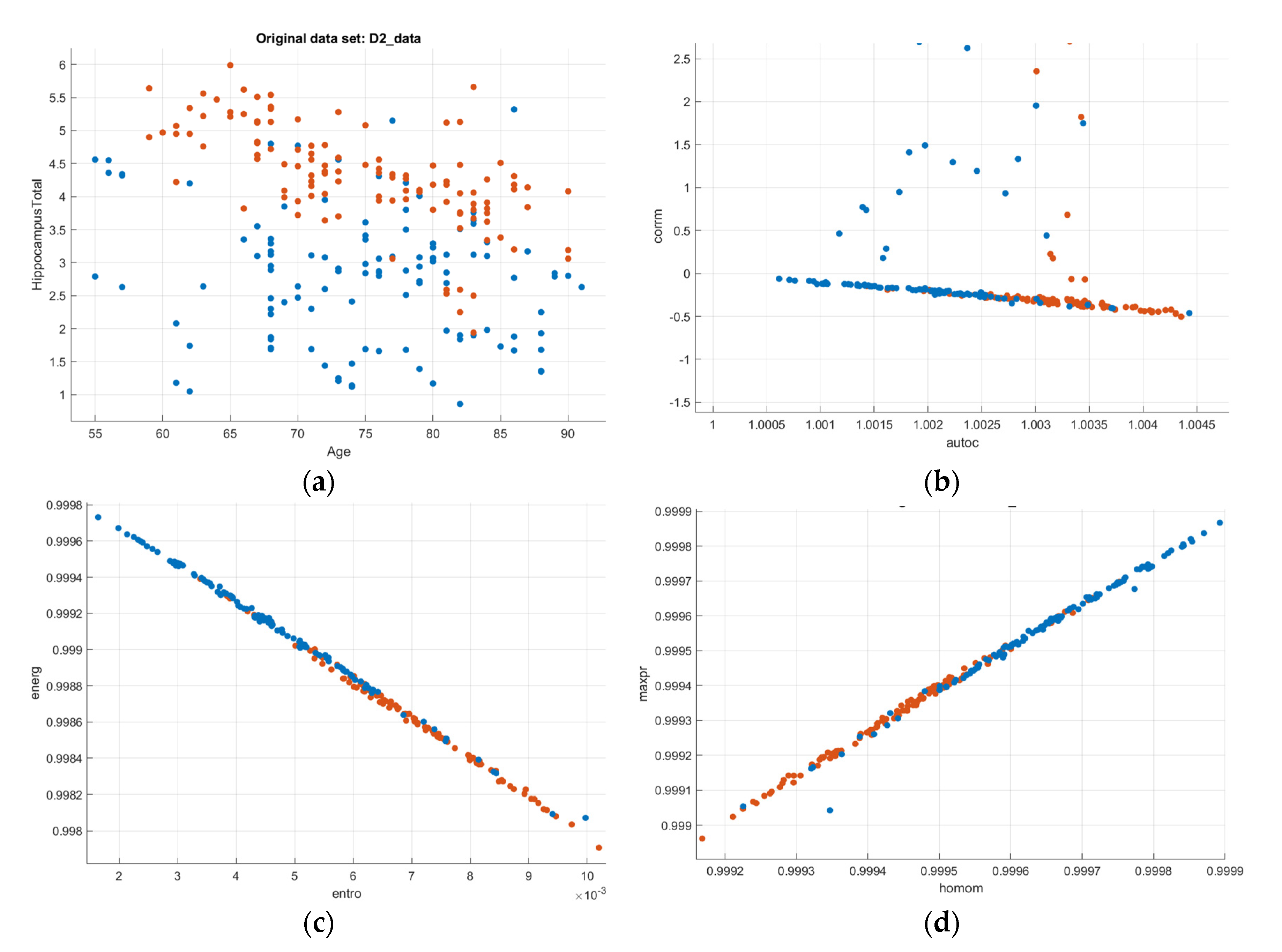
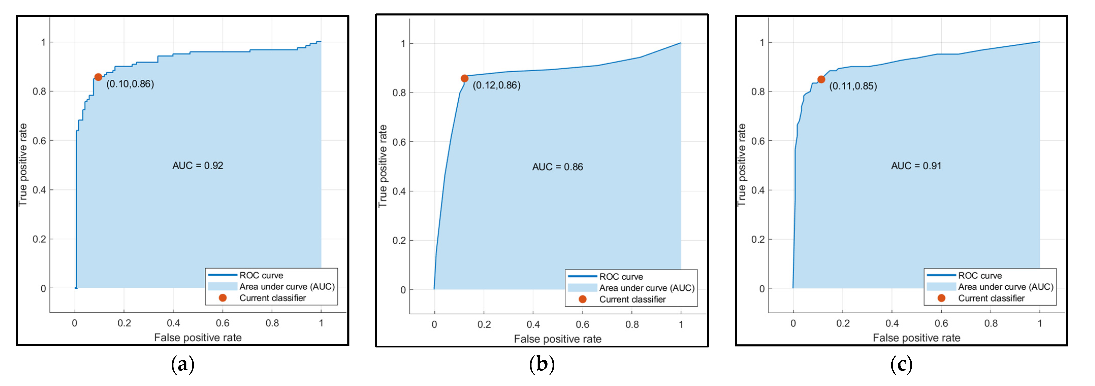
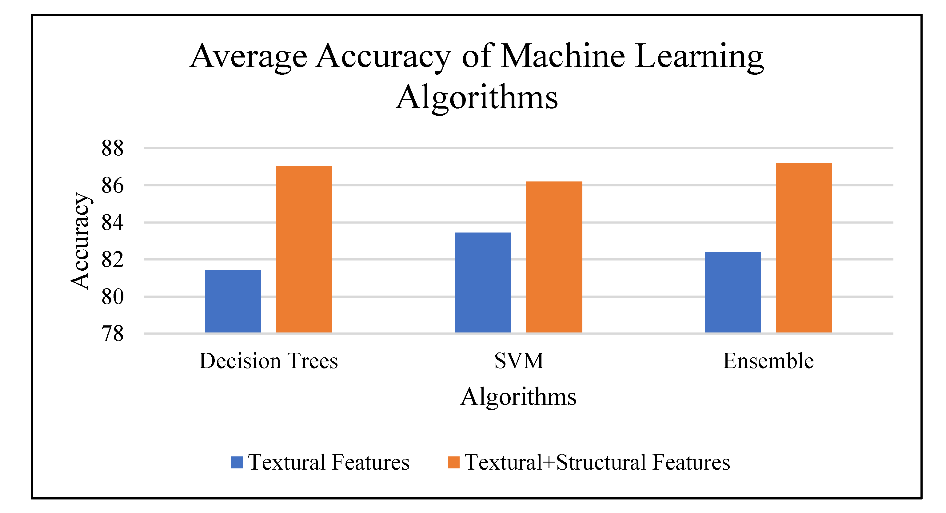
One of the most common problems with decision trees is overfitting. If no limit is given to the algorithm, it might give 100% training accuracy by creating a different node for each observation. Random forest, also called Ensemble Bagged trees, reduces overfitting in decision trees by combining multiple trees and selecting the best performance. First, the dataset is divided into N samples, and then a common learning rule is used for each sample; the prediction generated from this step is then combined using voting or by taking the average as, shown in Figure 9 [26,27].

3. Results

After obtaining the segmented hippocampus, 20 GLCM features were extracted with d = 1 and 2 for all the 13 possible directions, of which 8 (Autocorrelation, Energy, Entropy, Homogeneity, Maximum Probability, Correlation, and Information measure of correlations 1 and 2) were deemed to contribute the most to the classification by obtaining their feature score, and later analysis methods were shortlisted based on their GLCM feature score. After running GLCM on the dataset, 20 features were generated; however, the accuracy of the machine learning technique was relatively low. The lower accuracy was due to the dataset’s more considerable variance; it had a few factors contributing to randomness; therefore, those specific attributes were removed. An F-type statistic test was employed, which analyses the variance of two dataset means to eliminate the implausible values. It provided the standard deviation value, which explained the variance between datasets, resulting in reduced accuracy. This finding of the F value of statistical attributes aided in eliminating features that were not viable. Age and structural data such as hippocampus volume were included in the dataset for comparison analysis, in addition to these 8 GLCM features.

The research implementation platforms used python libraries and MATLAB. The classification model was trained using three different machine learning algorithms. SVM, Decision Trees, and Ensemble Bagged Trees were the models used (another name for Random Forest classifier). The dataset was taken into consideration when selecting these models. The classification was performed without setting advanced optimization techniques. Since the training dataset was limited (234), a classifier that can perform better with fewer data had to be chosen. The dataset with a clear separation between its classes performed well with SVM. Figure 10 gives the notion that for any machine learning algorithm, if the training and testing data was linearly separable, then the algorithms performed better than other nonlinear dataset classifiers. When instances of both the classes could be easily separated either by a straight line or nonlinearly, SVM became a suitable option for such data points. The scatter plot of several input features indicated that SVM would better fit the data set than other classifiers. SVM used a hard margin because the data was linearly separable. The regularization parameter (lambda) served as a degree of importance that was given to missclassifications. SVM posed a quadratic optimization problem that looks for maximizing the margin between both classes and minimizing the amount of missclassifications. The reason for choosing SVM, Decision Trees, and random forests is because of their implementation simplicity and relatively better model accuracy. Logistic regression, artificial neural networks, and nonlinear SVM work better when the data is nonlinear [28,29,30].

The number of trees in the Random Forest depends on the number of rows in the data set. In the case of a random forest, hyper parameters include the number of decision trees in the forest and the number of features considered by each tree when splitting a node. (The parameters of a random forest are the variables and thresholds used to split each node learned during training) [31].

Decision trees, which are also supervised learning algorithms, are another algorithm utilized in this section. The key reason for utilizing this technique is that it eliminates the requirement for the normalization of datasets. The dataset used has different scales for some attributes, therefore using this technique eliminates normalization.

Random Forest, also known as Ensemble Bagged Tree, is the third and final algorithm. It is a Decision Trees extension. It selects the best model from a set of uncorrelated decision tree classifiers. It takes longer to train than the other two algorithms, but it produces higher accuracy than the Decision Trees algorithm.

As per the data points generated from our dataset, Decision Trees, SVM, and Random Forest classifiers were chosen as they are simpler and more accurate as compared to other machine learning classifiers [32]. The dataset has linear boundaries and hence was better suited for the selected classifiers.

The confusion Matrix for the SVM, Decision Trees and Ensemble are illustrated in Figure 11.

The accuracy of the Decision Trees, SVM, and Ensemble models are shown in

Table 4. Classification accuracy based on structural data of the subjects.

Sr. No	Model	Classification Accuracy (%)
1	Decision Trees	86.8
2	SVM	87.2
3	Ensemble	86.3

. Only the volume and age were used as input features in these models. SVM outperformed the other two models in terms of accuracy. After observing the scatter plot of age and volume in Figure 10a, volume was the factor due to which SVM had superior accuracy. Figure 12 shows the Receiver Operating Characteristics (ROC) curve for SVM, Decision Trees, and Ensemble techniques.

From Figure 10b, the autocorrelation for AD patients was lower than compared to CN subjects. The uniformity in volumes of AD patients was higher than that of CN subjects, and the difference between neighbouring pixels was lower than that of CN subjects, as can be observed from Figure 10c. The randomness of intensity distribution was high for CN and was low for AD subjects. AD subjects had slightly more linear structures compared to CN. Figure 13 shows the comparative analysis of the volume data between AD and CN groups and it is seen that there is a noticeable distinction among the data samples.

In the next phase, classification models were trained only on the GLCM characteristics that had been identified. For textural features, Ensemble provided the highest accuracy (85%) at d = 1 and direction (d, d, 0), while Decision Trees was least accurate at d = 2 in direction (d, d, d). One evident finding from the accuracy table is that as the GLCM distance parameter was increased, the model’s accuracy decreased since average accuracy dropped from 82.60% to 82.23% for textural features. The right and left hippocampus were exceptionally small in the MRI, and as the distance parameter was increased, the quality of the GLCM matrix decreased due to its small dimensions; hence the distance was limited to d = 2. While the model was trained with eight GLCM features, i.e., Textural data, the results produced were unsatisfactory as it had less accuracy than the results produced with Textural and Structural Data.

Table 5. Classification accuracy with Textural and Structural data as input.

Distance and Directions		Classification Model Accuracy
		With Textural Data Only			With Textural and Structural Data
		Decision Trees	SVM	Ensemble	Decision Trees	SVM	Ensemble
d = 1	011	81.6	82.5	82.1	86.8	85.9	84.6
	100	81.2	84.6	82.9	88	86.8	88.5
	101	82.9	82.9	83.8	86.3	85.5	86.8
	110	82.5	84.2	85	85.9	87.2	87.6
	111	79.5	83.3	82.1	86.3	87.2	86.8
	11–1	79.9	82.1	80.3	88	85.5	90.2
	001	82.5	83.3	82	88.5	86.6	86.3
	01–1	82.9	83.3	82.9	88	86.8	86.3
	010	80.8	84.2	83.8	85.9	85.9	88
	10–1	81.2	83.8	81.6	88.5	85.9	88.9
	−11–1	82.1	84.2	82.9	86.3	86.3	86.8
	−110	82.9	84.2	82.5	88	86.3	87.6
	−111	81.6	84.6	80.8	88.9	85.9	86.8
d = 2	022	81.6	81.2	83.8	85.9	85.9	84.6
	200	80.3	85.9	81.6	85	85.5	86.3
	202	80.3	83.3	84.2	87.2	86.8	86.8
	220	81.6	84.2	81.2	88	86.8	88
	222	79.1	82.9	80.3	87.2	85.9	88.5
	22–2	79.9	82.1	82.9	88	86.8	86.3
	002	80.8	83.3	81.6	88.5	85	87.2
	02–2	82.5	82.5	79.9	85.9	87.2	86.3
	020	82.5	83.8	83.8	88.9	86.3	87.6
	20–2	80.8	84.2	80.8	84.2	85.9	87.6
	−22–2	83.3	84.2	84.2	85	85.5	88
	−220	80.3	84.2	82.9	86.3	86.3	88.5
	−222	82.1	80.8	82.1	87.2	85.5	85.5

represents the classification accuracy with Textural and structural data as input.

The texture features were merged with volume and age data. While the model was trained just on GLCM features, accuracy ranged from 79.1% to 85%. When only volume data was provided, the maximum accuracy was 87.2%. When the GLCM features dataset was paired with volume data, including the patient’s age and hippocampal volume, the accuracy improved up to 90.2%. The Ensemble Bagged Trees algorithm performed the best with the highest accuracy; one factor for better performance was the additional variables provided for the dataset. By including the structural data, a 4.38% improvement was observed on average.

The combination of features produce improvement by 4.38% on the structural data. Hence, it was observed as a better fit for the dataset. Figure 14 shows average accuracy for top performing machine learning algorithms applied on the data set.

Table 6. Classification accuracy based on texture analysis and machine learning techniques.

Author	Structure	Texture Analysis Method (Features)	Machine Learning Technique	Accuracy (%)
Xiao, Z. et al. [6]	Brain	GLCM, Gabor filter	SVM	For AD-CN data: 85.71
Oishi, K. et al. [33]	Gray Matter, White Matter, Cerebral Spinal Fluid and Background	Coefficient of Probability Changes	SVM	Maximum: 95 Average: 70
Kumar, K. et al. [34]	Brain	GLCM	k-NN	74.73
Luk, C.C. et al. [35]	Brain	3D GLCM	-	Maximum: 90.5 Average: 76
Chaddad, A. et al. [36]	Brain	3D GLCM	Ensemble	74.19
Madusanka, N. et al. [37]	Hippocampus	3D GLCM	SVM	86.61
Ranjbar, S. et al. [38]	Hippocampus	Hippocampal Volume	Diagonal Quadratic Discriminant Analysis (Naïve Bayes)	89

summarizes the classification accuracy based on texture analysis and machine learning techniques.

4. Conclusions

AD is one of the world’s leading causes of death from neurological disorders. The number of people with Alzheimer’s is steadily rising over the world. The neurologist’s manual diagnosis approach for AD is time-consuming and may not always yield correct results. One of the most significant elements in using brain images to classify AD is feature extraction. It is revealed that all 20 features retrieved from the GLCM of the participants’ MRI are not required. It is observed that the crucial eight features contribute the most to the classification of the individuals using the F-type statistics test. According to the results, the classification accuracy declines as the distance between neighbouring pixels increases. The comparisons demonstrate that using structural data, textural data, and age as input combined improves classification accuracy. The top-performing algorithms were Ensemble and Decision Trees, with a classification accuracy of 90.2% and 88.5%, respectively, and SVM, with a classification accuracy of 87.2%. The subject classification was on par with research articles that have used feature extraction using various image processing techniques [39].

References

1. Li, F.; Liu, M. Alzheimer′s Disease Neuroimaging Initiative. A hybrid convolutional and recurrent neural network for hippocampus analysis in Alzheimer’s disease. J. Neurosci. Methods 2019, 323, 108–118. [Google Scholar] [CrossRef]
2. Dhikav, V.; Anand, K.S. Hippocampus in health and disease: An overview. Ann. Indian Acad. Neurol. 2012, 15, 239–246. [Google Scholar] [CrossRef] [PubMed]
3. Zhang, J.; Yu, C.; Jiang, G.; Liu, W.; Tong, L. 3D texture analysis on MRI images of Alzheimer’s disease. Brain Imaging Behav. 2011, 6, 61–69. [Google Scholar] [CrossRef] [PubMed]
4. Sivapriya, T.R.; Saravanan, V.; Thangaiah, P.R.J. Texture Analysis of Brain MRI and Classification with BPN for the Diagnosis of Dementia; Springer: Berlin/Heidelberg, Germany, 2011; pp. 553–563. [Google Scholar] [CrossRef]
5. Haralick, R.M.; Shanmugam, K.; Dinstein, I.H. Textural features for image classification. IEEE Trans. Syst. Man Cybern. 1973, SMC-3, 610–621. [Google Scholar] [CrossRef] [Green Version]
6. Xia, H.; Tong, L.; Zhou, X.; Zhang, J.; Zhou, Z.; Liu, W. Texture Analysis and Volumetry of Hippocampus and Medial Temporal Lobe in Patients with Alzheimer’s Disease. In Proceedings of the 2012 International Conference on Biomedical Engineering and Biotechnology, Macau, Macao, 28–30 May 2012; pp. 905–908. [Google Scholar] [CrossRef]
7. Mohanaiah, P.; Sathyanarayana, P.; Gurukumar, L. Image Texture Feature Extraction Using GLCM Approach. Int. J. Sci. Res. Publ. 2013, 3, 1–5. [Google Scholar]
8. Kusiak, J.W.; Izzo, J.A.; Zhao, B. Neurodegeneration in Alzheimer disease. Mol. Chem. Neuropathol. 1996, 28, 153–162. [Google Scholar] [CrossRef] [PubMed]
9. ADNI. Alzheimer’s Disease Neuroimaging Initiative. Available online: http://adni.loni.usc.edu/ (accessed on 9 July 2021).
10. Salunkhe, S.D.; Bachute, M.R. A Bibliometric Analysis on Recent Classification Techniques for Alzheimer’s Disease Publication: Library Philosophy and Practice; Digital Commons@University of Nebraska: Lincoln, NE, USA, 2021; Volume 5658. [Google Scholar]
11. Leandrou, S.; Lamnisos, D.; Kyriacou, P.A.; Constanti, S.; Pattichis, C.S. Comparison of 1.5 T and 3 T MRI hippocampus texture features in the assessment of Alzheimer’s disease. Biomed. Signal Process. Control 2020, 62, 102098. [Google Scholar] [CrossRef]
12. Larobina, M.; Murino, L. Medical Image File Formats. J. Digit. Imaging 2013, 27, 200–206. [Google Scholar] [CrossRef]
13. Ding, Y.; Zhang, C.; Lan, T.; Qin, Z.; Zhang, X.; Wang, W. Classification of Alzheimer’s disease based on the combination of morphometric feature and texture feature. In Proceedings of the 2015 IEEE International Conference on Bioinformatics and Biomedicine (BIBM), Washington, DC, USA, 9–12 November 2015; pp. 409–412. [Google Scholar]
14. Manjón, J.V.; Coupe, P. volBrain: An Online MRI Brain Volumetry System. Front. Aging Neurosci. 2016, 10, 30. [Google Scholar] [CrossRef] [Green Version]
15. Frisoni, G.B.; Jack, C.R., Jr.; Bocchetta, M.; Bauer, C.; Frederiksen, K.S.; Liu, Y.; Preboske, G.; Swihart, T.; Blair, M.; Cavedo, E.; et al. The EADC-ADNI harmonized protocol for manual hippocampal segmentation on magnetic resonance: Evidence of validity. Alzheimer’s Dement. 2015, 11, 111–125. [Google Scholar] [CrossRef] [Green Version]
16. Romero, J.E.; Coupe, P.; Manjón, J.V. HIPS: A new hippocampus subfield segmentation method. NeuroImage 2017, 163, 286–295. [Google Scholar] [CrossRef] [PubMed] [Green Version]
17. Avinbash Uppuluri. GLCM_Features4.m: Vectorized Version of GLCM_Features1.m [With Code Changes]. MATLAB Central File Exchange. Available online: https://www.mathworks.com/matlabcentral/fileexchange/22354-glcm_features4-m-vectorized-version-of-glcm_features1-m-with-code-changes (accessed on 29 May 2021).
18. NITRC: MRIcron: Tool/Resource Info. Available online: https://www.nitrc.org/projects/mricron (accessed on 9 July 2021).
19. Caballero, D. Feature extraction algorithms from MRI to evaluate quality parameters on meat products by using data mining. ELCVIA Electron. Lett. Comput. Vis. Image Anal. 2018, 16, 1–4. [Google Scholar] [CrossRef] [Green Version]
20. Lahmiri, S.; Shmuel, A. Performance of machine learning methods applied to structural MRI and ADAS cognitive scores in diagnosing Alzheimer’s disease. Biomed. Signal Process. Control 2019, 52, 414–419. [Google Scholar] [CrossRef]
21. Barburiceanu, S.; Terebes, R.; Meza, S. 3D Texture Feature Extraction and Classification Using GLCM and LBP-Based Descriptors. Appl. Sci. 2021, 11, 2332. [Google Scholar] [CrossRef]
22. Soh, L.-K.; Tsatsoulis, C. Texture analysis of SAR sea ice imagery using gray level co-occurrence matrices. IEEE Trans. Geosci. Remote. Sens. 1999, 37, 780–795. [Google Scholar] [CrossRef] [Green Version]
23. Cortes, C.; Vapnik, V. Support-vector networks. Mach. Learn. 1995, 20, 273–297. [Google Scholar] [CrossRef]
24. Wu, X.; Kumar, V.; Quinlan, J.R.; Ghosh, J.; Yang, Q.; Motoda, H.; McLachlan, G.J.; Ng, S.K.; Liu, B.; Yu, P.S.; et al. Top 10 algorithms in data mining. Knowl. Inf. Syst. 2007, 14, 1–37. [Google Scholar] [CrossRef] [Green Version]
25. Nagawa, K.; Suzuki, M.; Yamamoto, Y.; Inoue, K.; Kozawa, E.; Mimura, T.; Nakamura, K.; Nagata, M.; Niitsu, M. Texture analysis of muscle MRI: Machine learning-based classifications in idiopathic inflammatory myopathies. Sci. Rep. 2021, 11, 9821. [Google Scholar] [CrossRef]
26. Ho, T.K. Random decision forests. In Proceedings of the 3rd International Conference on Document Analysis and Recognition, Montreal, QC, Canada, 14–16 August 1995. [Google Scholar] [CrossRef]
27. Bachute, M.; Vyas, N.; Modi, K.; Khanna, S.; Katpatal, C. Bibliometric Review on Classification of Alzheimer’s Disease Library Philosophy and Practice; Digital Commons@University of Nebraska: Lincoln, NE, USA, 2020; Volume 4843. [Google Scholar]
28. Raut, A.; Dalal, V. A machine learning based approach for detection of alzheimer’s disease using analysis of hippocampus region from MRI scan. In Proceedings of the 2017 International Conference on Computing Methodologies and Communication (ICCMC), Erode, India, 18–19 July 2017; pp. 236–242. [Google Scholar]
29. Fan, Z.; Xu, F.; Qi, X.; Li, C.; Yao, L. Classification of Alzheimer’s disease based on brain MRI and machine learning. Neural Comput. Appl. 2019, 32, 1927–1936. [Google Scholar] [CrossRef]
30. Stanzione, A.; Cuocolo, R.; Cocozza, S.; Romeo, V.; Persico, F.; Fusco, F.; Longo, N.; Brunetti, A.; Imbriaco, M. Detection of Extraprostatic Extension of Cancer on Biparametric MRI Combining Texture Analysis and Machine Learning: Preliminary Results. Acad. Radiol. 2019, 26, 1338–1344. [Google Scholar] [CrossRef]
31. Yasar, H.; Ceylan, M. A novel comparative study for detection of Covid-19 on CT lung images using texture analysis, machine learning, and deep learning methods. Multimed. Tools Appl. 2020, 80, 5423–5447. [Google Scholar] [CrossRef] [PubMed]
32. Yao, J.; Dwyer, A.; Summers, R.M.; Mollura, D.J. Computer-aided Diagnosis of Pulmonary Infections Using Texture Analysis and Support Vector Machine Classification. Acad. Radiol. 2011, 18, 306–314. [Google Scholar] [CrossRef] [Green Version]
33. Fuse, H.; Oishi, K.; Maikusa, N.; Fukami, T. Japanese Alzheimer’s Disease Neuroimaging Initiative. Detection of alzheimer’s disease with shape analysis of MRI images. In Proceedings of the 2018 Joint 10th International Conference on Soft Computing and Intelligent Systems (SCIS) and 19th International Symposium on Advanced Intelligent Systems (ISIS), Toyama, Japan, 5–8 December 2018; pp. 1031–1034. [Google Scholar] [CrossRef]
34. Kavin Kumar, K.; Devi, M.; Maheswaran, S. An efficient method for brain tumor detection using texture features and SVM classifier in MR images. Asian Pac. J. Cancer Prev. APJCP 2018, 19, 2789. [Google Scholar]
35. Luk, C.C.; Ishaque, A.; Khan, M.; Ta, D.; Chenji, S.; Yang, Y.-H.; Eurich, D.; Kalra, S. Alzheimer’s disease: 3-Dimensional MRI texture for prediction of conversion from mild cognitive impairment. Alzheimer’s Dement. Diagn. Assess. Dis. Monit. 2018, 10, 755–763. [Google Scholar] [CrossRef] [PubMed]
36. Chaddad, A.; Zinn, P.O.; Colen, R.R. Radiomics texture feature extraction for characterizing GBM phenotypes using GLCM. In Proceedings of the 2015 IEEE 12th International Symposium on Biomedical Imaging (ISBI), Brooklyn, NY, USA, 16–19 April 2015; pp. 84–87. [Google Scholar] [CrossRef]
37. Madusanka, N.; Choi, Y.Y.; Choi, K.Y.; Lee, K.H.; Choi, H.K. Hippocampus Segmentation and Classification in Alzheimer’s Disease and Mild Cognitive Impairment Applied on MR Images. J. Korea Multimed. Soc. 2017, 20, 205–215. [Google Scholar] [CrossRef]
38. Ranjbar, S.; Velgos, S.N.; Dueck, A.C.; Geda, Y.E.; Mitchell, J.R.; Alzheimer’s Disease Neuroimaging Initiative. Brain MR radiomics to differentiate cognitive disorders. J. Neuropsychiatry Clin. Neurosci. 2019, 31, 210–219. [Google Scholar] [CrossRef]
39. Karim, R.; Shahrior, A.; Rahman, M.M. Machine learning-based tri-stage classification of Alzheimer’s progressive neurodegenerative disease using PCA and mRMR administered textural, orientational, and spatial features. Int. J. Imaging Syst. Technol. 2021. [Google Scholar] [CrossRef]
Figure 1. Process flow.
Asi 04 00049 g001
Figure 2. Functional block scheme of volBrain.
Asi 04 00049 g002
Figure 3. Winterburn segmentation protocol obtained from volBrain.
Asi 04 00049 g003
Figure 4. Segmented Hippocampus volume viewed in MATLAB.
Asi 04 00049 g004
Figure 5. Representation of Volumetric Structure in 3D with grey intensities.
Asi 04 00049 g005
Figure 6. 13 directions for 3D GLCM.
Asi 04 00049 g006
Figure 7. SVM classification scheme.
Asi 04 00049 g007
Figure 8. Decision Trees classification scheme.
Asi 04 00049 g008
Figure 9. Ensemble classification scheme.
Asi 04 00049 g009
Figure 10. Scatter–plot representation of the GLCM features (AD-Blue, CN-Orange): (a) Age vs. Hippocampus Volume; (b) Autocorrelation vs. Correlation; (c) Entropy vs. Energy; (d) Homogeneity vs. Maximum Probability; (e) Information measures of correlation 1 and 2.
Asi 04 00049 g010aAsi 04 00049 g010b
Figure 11. Confusion Matrix for (a) SVM, (b) Decision Tree, and (c) Ensemble.
Asi 04 00049 g011
Figure 12. ROC curve for (a) SVM (b) Decision Trees and (c) Ensemble.
Asi 04 00049 g012
Figure 13. Comparison of volume data between AD and CN groups.
Asi 04 00049 g013
Figure 14. Average accuracy for top-performing machine learning algorithms.
Asi 04 00049 g014