Abstract
The objective of this work is the financial optimization of a solar-driven organic Rankine cycle. Parabolic trough solar collectors are used as the most mature solar concentrating system and also there is a sensible storage system. The unit is examined for the location of Athens in Greece for operation during the year. The analysis is conducted with a developed dynamic model in the program language FORTRAN. Moreover, a developed thermodynamic model in Engineering Equation Solver has been used in order to determine the nominal efficiency of the cycle. The system is optimized with various financial criteria, as well as with energy criteria. The optimization variables are the collecting area and the storage tank volume, while the nominal power production is selected at 10 kW. According to the final results, the minimum payback period is 8.37 years and it is found for a 160 m2 collecting area and a 14 m3 storage tank, while for the same design point the levelized cost of electricity is minimized at 0.0969 € kWh−1. The maximum net present value is 123 k€ and it is found for a 220-m2 collecting area and a 14-m3 storage tank volume. Moreover, the maximum system energy efficiency is found at 15.38%, and, in this case, the collecting area is 140 m2 and the storage tank volume 12 m3. Lastly, a multi-objective optimization proved that the overall optimum case is for a 160-m2 collecting area and a 14-m3 storage tank.
1. Introduction
Solar energy utilization is vital for facing important issues of our society such as global warming, fossil fuel depletion and increasing energy needs [1,2,3]. Concentrating solar power (CSP) is an important weapon for producing electricity which is the most valuable energy demand because it can cover numerous needs. Thus, a lot of research has been focused on power production with the use of solar concentrating systems [4,5].
Parabolic trough solar collector (PTC) is the most mature solar concentrating technology [6] and thus it is usually selected in CSP. Moreover, this technology has a reasonable cost, especially in systems with great scale. One of the most usual power blocks which can be coupled to the CSP is the Rankine cycle. For PTC, the organic Rankine cycle (ORC) is usually selected due to the best compatibility between the operating temperature levels of the PTC and the ORC [7,8].
In the literature, many studies examine the solar-driven ORC with PTC. Quoilin et al. [9] performed a study about a system with PTC and ORC that operates with R245fa and presented system efficiency up to 8%. Astolfi et al. [10] examined an ORC that is driven by PTC and geothermal energy. This system presents a 9.4% system efficiency and levelized cost of electricity (LCOE) from 0.145 up to 0.280 €·kWh−1. Bellos and Tzivanidis [11] examined the combinations of PTC with waste heat in an ORC. They found that the best working fluid is toluene and the system efficiency can range from 11.6% up to 19.7%. He et al. [12] investigated a system with PTC coupled to a regenerative ORC. They found that the system efficiency is close to 15%, and they studied the system parametrically. The main parameters of their work were the storage tank volume and the mass flow rate of the heat transfer fluid. Desai and Bandyopadhyay [13] compared the use of PTC and linear Fresnel reflectors (LFR) coupled to ORC. They studied different working fluids and they found the most suitable working fluids to be R113, isohexane, hexane, benzene and cyclohexane. They concluded that the system with PTC has higher efficiency, which is close to 20% and the LCOE is about 0.4 € kWh−1. At this point, it is important to explain that the LCOE is a critical parameter that shows how the real is the cost of the produced electricity. In the cases that the LCOE is lower than the electricity price, then the investment is viable. In cases with high LCOE, there is a need for a subsidy for creating a viable investment.
Tzivanidis et al. [14] studied the use of PTC in order to feed an ORC in the Greek climate. They studied four typical days and they extended the results for all the year. They found that there is a need for 25,000 m2 of PTC in order to feed a system with nominal power at 1 MW. The optimum ratio of the collecting area to storage tank volume was found at 80 m2/m3, and, for this case, the system efficiency is 13.46% and the payback period is at 9 years. Askari-Asli Ardeh et al. [15] examined a PTC with a V-shape cavity coupled to an ORC. They found that this unit is able to lead to a payback period lower than 9 years and to a system efficiency of about 25% in optimal design. Chacartegui et al. [16] investigated a system with PTC and ORC and they gave the emphasis in the storage system. They found that the toluene is the best working fluid which leads to an LCOE at 0.17 €·kWh−1. Casati et al. [17] performed a work about solar-driven ORC with different storage systems. They concluded that the use of storage is important and it has to be used in these systems. Moreover, their study case was for a system with 100 kW nominal power and 18% system efficiency. Bellos and Tzivanidis [18] studied the idea of using a nanofluids-based PTC in a solar-ORC. They found that toluene is the best organic fluid, while the thermal oil/CuO is the best nanofluid. The nanofluid-based system presents 20.1% system efficiency, which is 1.75% higher than the system with pure thermal oil in the solar field.
The previous literature review indicates the high interest of the ORCs driven by PTC. In this direction, this work examines a system with PTC, a sensible storage system and ORC operating with toluene. The system is examined with a developed dynamic model in the programming language FORTRAN. The thermodynamic analysis has been performed with a developed model in Engineering Elution Solver (EES) [19]. The system is investigated for the location of Athens in Greece for operation during the year. The novelty of this work is the optimization of these systems under different criteria and the comparison of the different optimum designs. Furthermore, there is an extra multi-objective optimization procedure that is able to determine the global optimum design of the solar-driven ORC. The difference of this work compared to previous studies is based on the detailed optimization analysis and on the use of the proper sunny days for every month in order to find representative results. The comparison of the different optimum designs is critical in order to know how these systems have to be designed in accordance with the evaluation criteria in any case. The emphasis is given in the optimization with different financial criteria, such as payback period, net present value, and the levelized cost of electricity. Moreover, energy efficiency is used as an optimization criterion in this work. The optimization variables are the collecting area and the storage tank volume, which are the main parameters for the solar field design. Lastly, it is also important to state that a parametric analysis is conducted before the optimization procedure, in order to make clear the way that every parameter influences the financial and energy indexes.
2. Material and Methods
2.1. The Examined System
The examined system is depicted in Figure 1. There are PTCs, a storage tank and an ORC. The working fluid in the solar field and the tank is Therminol VP-1 [20], which is a usual selection. The storage tank includes thermal oil and stores sensible heat. The maximum temperature level in the system is selected at 400 °C [20]. The thermal loss coefficient of the storage tank (UT) is selected at 0.5 W m−2·K−1 [21] and the specific mass flow rate in the PTC (mcol/Ac) is selected at 0.02 kg s−1·m−2 [22]. The ORC operates with toluene as the working fluid, which is a proper selection for efficiency according to the literature [16,18,23]. The ORC is a regenerative cycle which includes a recuperator.
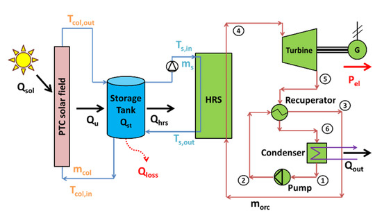
Figure 1.
The examined solar-driven organic Rankine cycle (Parabolic trough solar collector (PTC), tank, organic Rankine cycle (ORC)).
2.1.1. Solar Field Modeling
The thermal efficiency of the PTC (ηth,col) is calculated as below. This formula regards the EuroTrough module, which is assumed to be used in this work [24,25].
The PTC incident angle modifier (K) for the EuroTrough module is calculated according to the next formula [26]:
The useful heat production of the PTC (Qu) is calculated as:
The solar direct beam irradiation on the PTC (Qsol) is given as:
The thermal efficiency of the PTC (ηth,col) is defined as:
In this work, the inlet oil temperature in the PTC is equal to the mean storage tank temperature (Tcol,in = Tst) and the heat source temperature in the inlet HRS inlet is equal to the mean storage tank temperature (Ts,in = Tst). About the storage tank, the general energy balance is given as:
Moreover, it has to be said that the storage sensible heat (Qst) can be expressed as:
Practically, in this work, the storage system is modeled by using the energy balance of Equation (6). Equation (7) shows the way that the stored energy can be expressed in terms of a temperature increase in the tank. In this work, the tank is modeled by one thermal zone, which is an assumption of this study. The temperature is assumed to be uniform in the tank in every time step. It has to be said that the examined storage tanks have relatively high storage capacity and so there are not high fluctuations in the temperature during the day inside the tank, something that makes possible the modeling with a single thermal zone.
The thermal losses of the storage tank (Qloss) are calculated as below:
In this work, a cubic tank is assumed and its area is connected with the storage tank volume as below:
The heat input in the heat recovery system (HRS) is calculated as:
2.1.2. Organic Rankine Cycle Modeling
The work production in the ORC turbine shaft (WT) is given as:
The power demand of the pumping work (Wp) is given below:
The motor efficiency (ηmotor) is selected at 80% in this work.
The isentropic efficiency of the turbine (ηis,T) is selected at 85% [27] and its definition is given below. It has to be said that the selected value is a relatively high value and it corresponds to a well-designed expansion device in order to achieve high system efficiency.
The ORC net electricity production (Pel) is given below:
The electrical generator efficiency (ηg) is selected at 98% and the mechanical efficiency (ηm) at 99% which are reasonable values.
The ORC efficiency is defined as below:
The system instantaneous energy efficiency (ηsys) is defined as:
Moreover, the yearly energy efficiency of the system (ηen-y) is defined as below:
The yearly electricity production (Eel) and the yearly solar potential (Esol) are defined as:
Practically, in this work, every month is examined by using a typical day. For every month, a specific number of sunny days (SD) are used in order to take into account only the days with the potential for exploitation of the beam irradiation. The sunny days from January up to December are the following: 13, 10, 15, 18, 20, 22, 29, 29, 20, 18, 17 and 15, respectively [28]. In total, there are 218 sunny days during the year, which is a reasonable number of days. These data have been taken by using statistical results for Athens, Greece [29,30,31]. More specifically, the used number of sunny days for every month has been found after calculating the average monthly number of sunny days for the last five years [30].
2.1.3. Financial Analysis Formulation
The system investment cost (C0) is calculated as:
The yearly system cash flow (CF) can be written as:
The operation and maintenance cost (KO&M) is estimated as 1% of the capital cost:
The net present value (NPV) of the investment is calculated as:
where the equivalent project life (R) is expressed as:
The simple payback period (SPP) is defined as:
The payback period (PP) is calculated as:
The levelized cost of electricity (LCOE) can be calculated as below:
Table 1 includes the data of the financial analysis [14,32,33]. It has to be said that, according to Ref. [32], the electricity price in Greece for a CSP with thermal storage is 0.28485 € kWhel−1, which is a very satisfying value.

Table 1.
Data for financial analysis [28,33].
2.2. Procedure Description
The first part of this work is the development of a thermodynamic model in Engineering Equation Solver (EES) [19] in order to determine the ORC efficiency. The working fluid is toluene and this is a suitable selection for high-temperature levels in the range of 300–400 °C. Table 2 includes the main data of the ORC and more information about these values can be found in other previous studies [14,18,23,33].
Table 2.
Parameters of the organic Rankine cycle.
The next stage in this work is the dynamic investigation of the examined system. In this analysis, a program is developed in the programming language FORTRAN. This model studies 12 different days, one for every month and then the all year period can be studied. More specifically, for every month, the proper number of sunny days is used in order to take into consideration the proper solar potential for every month. The weather data regard the location of Athens in Greece and these data can be found in the following Refs. [21,28].
In the developed code, the time step is selected at 1 min after sensitivity analysis. For every month, the typical day is converged after an iterative process. In this process, the day is faced as 7 identical days that are solved the one after the other. So, the last day of this set is the converged day, which corresponds to reality.
The goal of this work is the optimization of the examined system. The optimization variables are the collecting area (Ac) and the storage tank volume (V). Table 3 includes data about the optimization variables. The collecting area is studied from 100 up to 300 m2 with a step of 20 m2, while the storage tank volume from 10 up to 30 m3 with a step of 2 m3. In total, 121 cases are examined by investigating all the possible combinations of collecting areas and storage tank volumes. These 121 cases are evaluated with different criteria, and, in every case, the optimum case is selected. This is a simple optimization procedure methodology but it easy to be done due to the use of only two optimization variables and to the low computational cost of every run. The optimization goals of this work are the following: the maximization of the NPV, the minimization of the payback period, the minimization of the LCOE and the maximization of the yearly energy efficiency. In every case, only one goal is used and so this work includes single-objective optimization results.
Table 3.
Data about the optimization variables.
Moreover, the last step in this work is a multi-objective optimization procedure that is conducted in order to determine the overall optimum design. The NPV and the energy efficiency are selected as the proper criteria in order to perform this multi-objective analysis. One financial index and one energy index are combined in order to give an optimum design that follows both financial and energy efficiency criteria. The goal of this procedure is to evaluate the 121 design cases and to find the one that has the minimum dimensionless geometric distance from the ideal point. This procedure has also been followed in other literature studies [33]. The optimization variable (F) is defined as below:
Practically, the included parameters of the multi-objective evaluation procedure have to be maximized and so there is a Pareto-front theoretical line. The overall optimum choice is the design point of the Pareto-front, which has the minimum dimensionless geometrical distance by the ideal point which has as coordinates the maximum values of the NPV and the yearly energy efficiency. The use of dimensionless parameters makes the procedure to be fair and to give the same weights in both variables. The subscripts “min” and “max” indicate the minimum and maximum values, respectively, among the examined 121 cases.
3. Results and Discussion
3.1. Parametric Analysis
In the parametric analysis, we examine the impact of the collecting area and the storage tank on the system performance. The results are separated in energy results (Section 3.1.1) and financial results (Section 3.1.2). All the indexes are studied for different collecting areas and storage tank volumes. Figures with the collecting area in the horizontal axis and the storage tank volume in the horizontal axis are given separately in order to present the results in a detailed way.
3.1.1. Energy Analysis
The first examined index is electricity production, which is the most important parameter. Figure 2a shows that higher collecting increases electricity production on a yearly basis. However, after the 160 m2, the increasing trend of the curves reduces. Moreover, the curves for storage tanks between 16 and 30 m3 are extremely close to each other, while for smaller tanks the electricity production is generally lower. Another interesting result is that for small collecting areas, the optimum storage tanks are smaller. More specifically, Figure 2b indicates that for collecting areas of 100 and 120 m2, the optimum storage tank is the smallest examined (10 m3), while for higher collecting areas, the optimum volume increases. The results indicate that the optimum storage tank volumes generally range from 12 up to 16 m3 in order to have the maximum electricity production. The yearly production of electricity can reach up to 52.16 MWh for a 300-m2 collecting area and a 30-m3 storage tank volume, which indicates a system that operates about 60% of the year.
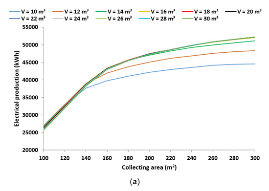

Figure 2.
Electrical production (a) for different collecting areas with the storage tank volume as the main parameter (b) for different storage tank volumes with the collecting area as the main parameter.
It is useful to note that a higher storage tank gives the possibility for greater storage capacity and so higher solar irradiation amounts to be used in the afternoon after the sunset. Especially in the summer, the higher storage tank volumes are critical in order not to reach the maximum temperature limit of 400 °C and so not to stop the system operation for some hours per day. On the other hand, an extremely great storage tank leads to high thermal losses due to the high outer tank surface. Moreover, a very huge tank creates difficulties in the operation during the winter because there is not the ability to reach the temperature limit of 334.7 °C for operation.
The next examined parameter is the yearly system efficiency. This fact shows the ratio of the produced electricity to the available solar irradiation of the examined days. Figure 3a illustrates that for every storage tank volume curve, there is a specific collecting area that maximizes energy efficiency. Generally, the maximum energy efficiency is found for collecting areas in the range from 120 to 140 m2. The maximum yearly system efficiency is 15.38% and it is found for a 140-m2 collecting area and a 12-m3 storage tank volume.
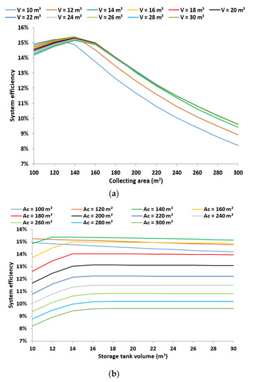
Figure 3.
System efficiency (a) for different collecting areas with the storage tank volume as the main parameter (b) for different storage tank volumes with the collecting area as the main parameter.
Figure 3b shows that there is an optimum collecting area that maximizes the energy efficiency for all the storage tanks volumes from 14 up to 30 m3. However, for the storage tanks of 100 and 120 m2, the tank volume is the minimum examined of 10 m3. At this point, it is critical to state that, in this work, the optimum collecting area for the smallest examined volumes is lower than 100 m2 and thus some curves have different shapes in the examined range. However, this fact does not play any role in the overall optimum choice because the optimum designs are included in the examined ranges of collecting areas and storage tank volumes.
3.1.2. Financial Analysis
The financial analysis is presented through some important indexes. Figure 4a,b shows results about the NPV. The NPV is an important parameter that shows the overall gain from the investment in all their lifetime. This parameter is usually used in the evaluation of the investments but it needs the use of some parameters, such as the discount factor and the project lifetime. These parameters are not known and they are estimated, something that makes the values of the NPV to be connected with the selection of some parameters. Figure 4a shows that the NPV is maximized for collecting areas in the range of 180 up to 240 m2. The overall maximum NPV is 15.71 k€ and it is found for a 220-m2 collecting area and a 14-m3 storage tank volume. Figure 4b indicates that the optimum storage tank volume is up to 14 m3. Generally, it has to be said that higher collecting leads to higher electricity production, but, after a limit, the gain in electricity is not so high for counterbalance the extra cost.
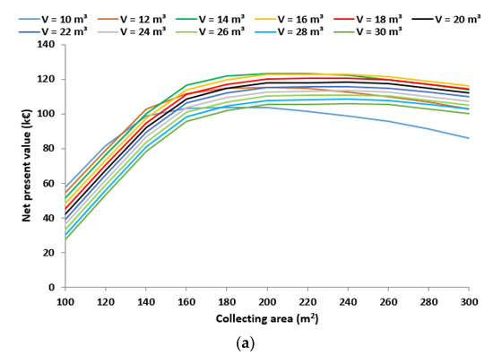
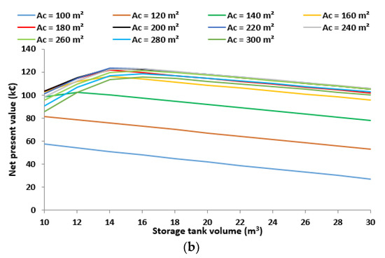
Figure 4.
Net present value (a) for different collecting areas with the storage tank volume as the main parameter (b) for different storage tank volumes with the collecting area as the main parameter.
Figure 5a,b shows the LCOE for the examined cases. Generally, the minimization of the LCOE is found for collecting areas close to 140 to 160 m2. For greater collecting areas, the LCOE increases and so the investment viability does not increase. The optimum storage tanks are about 12 to 14 m3. The minimum LCOE is 0.0969 € kWh−1 and it is found for a 14-m3 storage tank volume and a 160-m2 collecting area. Higher tank volumes are not beneficial for the investments and this fact has to be taken into account when these systems are designed. Generally, the LCOE has reasonable values that are lower than the electricity price. Thus, the investment of the solar-driven ORC is viable.
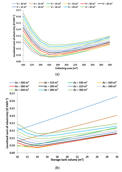
Figure 5.
Levelized cost of electricity (a) for different collecting areas with the storage tank volume as the main parameter (b) for different storage tank volumes with the collecting area as the main parameter.
Figure 6a,b illustrates the payback period, while Figure 7a,b illustrates the simple payback period. The results have similar trends for these indexes because these parameters show the same thing but for different scenarios. The payback period takes into account the discount factor while the simple payback period does not take into consideration any other external parameters. In other words, the payback period may be a more realistic parameter than the simple payback period but the payback period is influenced by an estimated parameter which is the discount factor. However, the optimization with these parameters leads to the same overall optimum system. Moreover, it is important to state that, in the present work, the minimization of the LCOE is matched with the minimization of the PP and SPP. The minimum payback period is 8.37 years and the minimum simple payback period of 7.30 years. These values are found for a 14-m3 storage tank volume and a 160-m2 collecting area.
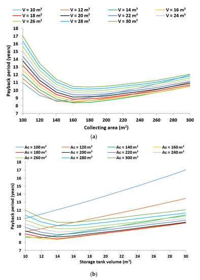
Figure 6.
Payback period (a) for different collecting areas with the storage tank volume as the main parameter (b) for different storage tank volumes with the collecting area as the main parameter.
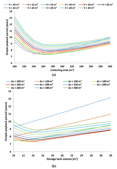
Figure 7.
Simple payback period (a) for different collecting areas with the storage tank volume as the main parameter (b) for different storage tank volumes with the collecting area as the main parameter.
3.2. Optimization Results
The optimization of the examined system is performed in various ways. In the first part, there are single-objective optimization procedures and in the second part, there is a multi-objective optimization procedure. Table 4, Table 5 and Table 6 show the optimization results with different criteria and more specifically for maximizing the energy efficiency, minimizing the payback period and maximizing the net present value respectively. It is critical to state that the minimization of the payback period leads to the minimization of the LCOE in all the examined cases and thus there is not a separate table for LCOE minimization. Moreover, Table 4, Table 5 and Table 6 include results about the optimum collecting areas, according to different criteria, for all the examined storage tank volumes. Moreover, the overall optimum values can be found in these tables by observing all the results together.
Table 4.
Optimum collecting areas for different storage tank volumes for maximizing energy efficiency.
Table 5.
Optimum collecting areas for different storage tank volumes for minimizing the payback period.
Table 6.
Optimum collecting areas for different storage tank volumes for maximizing the net present value.
Table 4 shows that the overall maximum yearly energy efficiency is 15.38% and it is found for a 140-m2 collecting area and a 12-m3 storage tank volume. In this case, the yearly electricity production is 38917 kWh, the payback period is 8.58 years, the yearly solar collector efficiency 52.22%, the LCOE is 0.0989 € kWh−1 and the NPV is 102.63 k€. Moreover, Table 5 proves that the overall minimum payback period is 8.37 years and it is found for a 160-m2 collecting area and a 14-m3 storage tank volume. In this case, the yearly electricity production is 43328 kWh, the yearly energy efficiency is 14.99%, the yearly solar collector efficiency 50.68%, the LCOE is 0.0969 € kWh−1 and the NPV is 116.29 k€. Furthermore, Table 6 shows that the overall maximum net present value is 123.21 k€ and it is found for a 220-m2 collecting area and a 14-m3 storage tank volume. In this case, the yearly electricity production is 48275 kWh, the yearly energy efficiency is 12.14%, the yearly solar collector efficiency 40.77%, the LCOE is 0.1025 € kWh−1 and the payback period 8.96 years.
So, it can be said that different optimization criteria lead to different optimum design parameters. Thus, an extra multi-objective optimization procedure is conducted. Figure 8 is a depiction of the multi-objective optimization procedure. The energy efficiency and the NPV are used as the two goals that have to be maximized. This procedure has an energetic and a financial index and thus it is interesting. Moreover, the optimum design points with these two criteria separately give different results and so the multi-objective optimization is emerging. It was found that the optimum design is the one with a 160-m2 collecting area and a 14-m3 storage tank. This design is the one that has been found to be the best one for minimizing both the payback period and the LCOE. Thus, it can be said that this design can be adopted as the overall optimum case for the present system. At this point, it is interesting to state that the found values of the LCOE are around 0.1 €/kWh. In the literature, the reported values are generally higher and thus this work shows that the optimization is able to significantly reduce the LCOE. More specifically, Astolfi et al. [11] found the LCOE to range from 0.145 up to 0.280 € kWh−1, Desai and Bandyopadhyay [13] found the LCOE around 0.4 € kWh−1 and Chacartegui et al. [16] calculated the LCOE at 0.17 € kWh−1. So, this work has to add to the literature promising results about the financial viability of the solar-driven ORC technology.
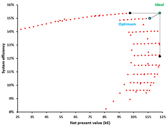
Figure 8.
Pareto-front and multi-objective optimization depiction with the system efficiency and the net present value as the optimization goals. (The black points are the side points, the green point is the ideal point and the blue point is the optimum point).
Another comment about the found results is that the cases with the higher collecting areas lead to lower solar field yearly efficiency. This is a reasonable result because a higher collecting area leads to higher operating temperatures and so the collector efficiency reduces due to the higher thermal losses. The ratio of the collecting area to the storage tank is found to be 11.43 m2/m3 in the overall optimum case. This value is different compared to another previous study of the same research team where this ratio was found 80 m2/m3 [15]. There are many reasons for this difference in the found values. First of all, in the present work, the cost of the electricity price is higher than the other study due to the respective difference in the legislation. Moreover, there are different weather data between these studies. This work uses 12 typical days for simulation all the year, while the analysis of Ref. [15] used four typical days. Moreover, there are some different points in the design of the ORC and of the storage tank modeling that can lead to different results.
3.3. Monthly Analysis
This section includes the results of the monthly performance of the examined system. The three different optimum designs, according to the criteria of Section 3.2, are included in the monthly analysis. Figure 9 regards the monthly electricity production, Figure 10 the monthly system efficiency and Figure 11 the monthly collector efficiency.
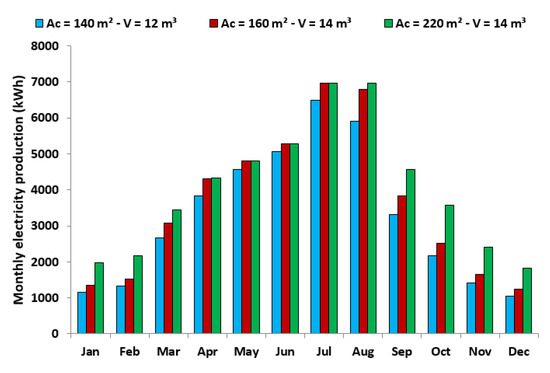
Figure 9.
Monthly electrical production for optimum cases (Ac = 140 m2 − V = 12 m3, Ac = 160 m2 − V = 14 m3, Ac = 220 m2 − V = 14 m3).
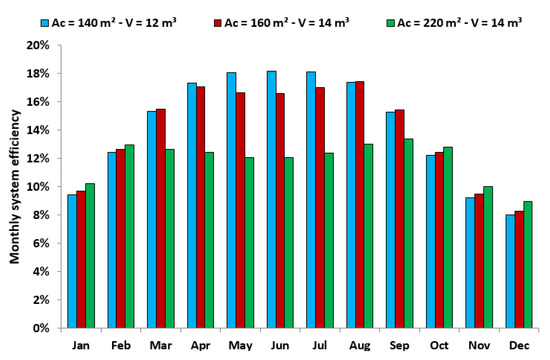
Figure 10.
Monthly system efficiency for optimum cases (Ac = 140 m2 − V = 12 m3, Ac = 160 m2 − V = 14 m3, Ac = 220 m2 − V = 14 m3).
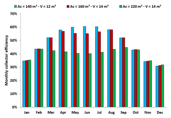
Figure 11.
Monthly collector efficiency for optimum cases (Ac = 140 m2 − V = 12 m3, Ac = 160 m2 − V = 14 m3, Ac = 220 m2 − V = 14 m3).
Figure 9 indicates that electricity production is at the maximum during the summer and especially in July and in August. Moreover, it is useful to state that the systems with higher collecting areas give higher electricity and it is more intense during the months with lower solar potential (e.g., winter). On the other hand, in July, the use of 160 and 220 m2 leads to the same electricity production because both areas are enough for operation during all the days due to the over-sizing of the system this month. However, this over-sizing is valid only for summer and not for the winter period, so, overall, the system is not oversized.
Figure 10 shows that higher collecting area leads to lower system efficiency because higher amounts of solar irradiation are not utilized, especially during the summer. However, during the winter months, the higher collecting area makes the system to operate more hours per day compared to the low area systems, something that makes it more efficient during the winter. Figure 11 indicates that higher collecting area leads to higher mean operating temperature and so to lower collector efficiency.
4. Conclusions
The objective of this work is the optimization of a solar-driven organic Rankine cycle that operates with toluene as the working fluid. Parabolic trough collectors coupled to a sensible storage system are used in order to feed the ORC for electricity production. The system is examined for all the years in the location of Athens in Greece. The analysis is conducted with a dynamic model that is programmed in FORTRAN. The thermodynamic data of the ORC have been taken by a developed thermodynamic model in Engineering Equation Solver (EES). The optimization variables are the collecting area and the storage tank volume. There are different optimization criteria that are mainly financial, as well as the system energy efficiency. Moreover, a multi-objective optimization procedure is performed. The most important conclusions of this work are summarized below:
- The maximum system energy efficiency is found at 15.38%, and, in this case, the collecting area is 140 m2 and the storage tank volume is 12 m3.
- The maximum net present value is 123 k€ and is found for a 220-m2 collecting area and a 14-m3 storage tank volume.
- The minimum payback period is 8.37 years and is found for a 160-m2 collecting area and a 14-m3 storage tank, while, for the same design point, the levelized cost of electricity is minimized at 0.0969 € kWh−1.
- The multi-objective optimization procedure proved that the optimum design is for a 160-m2 collecting area and a 14-m3 storage tank. Moreover, this design point is the optimum according to the payback period minimization and LCOR minimization criteria. Thus, this design is selected as the overall optimum choice.
- The monthly analysis indicates that higher electricity is produced during the summer and especially in July and in August. Moreover, the use of higher collecting areas leads to significant enhancement in electricity production, mainly in the winter period.
Author Contributions
Supervision, writing—review and editing, writing—original draft preparation, C.T.; conceptualization, methodology, investigation, writing—review and editing, writing—original draft preparation, E.B. All authors have read and agreed to the published version of the manuscript.
Funding
This research is co-financed by Greece and the European Union (European Social Fund ESF) through the Operational Programme, Human Resources Development, Education and Lifelong Learning, in the context of the project “Reinforcement of Postdoctoral Researchers 2nd Cycle” (MIS-5033021), implemented by the State Scholarships Foundation (IKΥ).
Acknowledgments
Evangelos Bellos would like to thanks the State Scholarships Foundation (IKΥ) for its financial support (MIS-5033021).
Conflicts of Interest
The authors declare no conflicts of interest.
Nomenclature
| Ac | Collecting area, m2 |
| AT | Storage tank outer area, m3 |
| cp | Specific heat capacity, kJ kg−1 K−1 |
| C0 | Capital cost, € |
| CF | Hourly cash flow, € h−1 |
| E | Yearly energy quantity, kWh |
| F | Objective function of dimensionless distance, - |
| Gb | Solar direct beam irradiation, W·m−2 |
| i | Counter, - |
| h | Specific enthalpy, kJ kg−1 |
| K | Incident angle modifier, - |
| Kcol | Specific collector cost, € m−2 |
| Kel | Electricity cost, € kWhel−1 |
| Korc | Specific cost of the organic Rankine cycle, € kWel−1 |
| KO&M | Yearly operating and maintenance cost, € |
| Ktank | Specific cost of the storage tank, € m−3 |
| LCOE | Levelized cost of electricity, € kWel−1 |
| m | Mass flow rate, kg s−1 |
| N | Project life, years |
| NPV | Net present value, k€ |
| P | Pressure, bar |
| Pel | Net electricity production, kW |
| PPhrs | Pinch Point, °C |
| PP | Payback Period, years |
| Q | Heat rate, kW |
| Qout | Heat rejection to the ambient, kW |
| r | Discount factor, % |
| R | Equivalent investment time, years |
| SD | Sunny days, days |
| SPP | Simple Payback Period, years |
| t | Time, hours |
| T | Temperature, °C |
| Tam | Ambient temperature, °C |
| UT | Thermal loss coefficient of the tank, W m−2·K−1 |
| V | Storage tank volume, m3 |
| Wp | Pumping work, kW |
| WT | Turbine work production, kW |
Greek Symbols
| ΔP | Pressure difference, bar |
| ΔΤsh | Superheating degree in the turbine inlet, °C |
| ΔTrc | Temperature difference in the recuperator, °C |
| ηen | Instantaneous energy efficiency, - |
| ηen-y | Yearly energy efficiency, - |
| ηis,T | Isentropic efficiency of the turbine, - |
| ηg | Generator efficiency, - |
| ηm | Mechanical efficiency, - |
| ηmotor | Motor efficiency, - |
| ηorc | Efficiency of the power block, - |
| ηth,col | Collector thermal efficiency, - |
| θ | Incident solar angle on the collector aperture, ° |
| ρ | Density, kg m−3 |
Subscripts and Superscripts
| col | Collector |
| col,in | Collector inlet |
| col,out | Collector outlet |
| con | Condenser |
| is | Isentropic |
| in | Inlet |
| hrs | Heat recovery system |
| loss | Thermal losses in the tank |
| max | Maximum |
| min | Minimum |
| opt | Optimum |
| orc | Fluid in the organic Rankine cycle |
| out | Outlet |
| s | Heat source |
| s,in | Heat source inlet |
| s,out | Heat source outlet |
| sat | Saturation in the heat recovery system |
| sol | Solar |
| st | Storage tank |
| T | Turbine |
| u | Useful |
Abbreviations
| CSP | Concentrating Solar Power |
| EES | Engineering Equation Solver |
| HRS | Heat Recovery System |
| ORC | Organic Rankine Cycle |
| PTC | Parabolic Trough Collector |
References
- Wang, F.; Cheng, Z.; Tan, J.; Yuan, Y.; Yong, S.; Liu, L. Progress in concentrated solar power technology with parabolic trough collector system: A comprehensive review. Renew. Sustain. Energy Rev. 2017, 79, 1314–1328. [Google Scholar]
- Mehmood, A.; Waqas, A.; Said, Z.; Rahman, S.M.A.; Akram, M. Performance evaluation of solar water heating system with heat pipe evacuated tubes provided with natural gas backup. Energy Rep. 2019, 5, 1432–1444. [Google Scholar] [CrossRef]
- Kasaeian, A.; Bellos, E.; Shamaeizadeh, A.; Tzivanidis, C. Solar-driven polygeneration systems: Recent progress and outlook. Appl. Energy 2020, 264, 114764. [Google Scholar] [CrossRef]
- Islam, M.T.; Huda, N.; Abdullah, A.B.; Saidur, R. A comprehensive review of state-of-the-art concentrating solar power (CSP) technologies: Current status and research trends. Renew. Sustain. Energy Rev. 2018, 91, 87–1018. [Google Scholar] [CrossRef]
- Pelay, U.; Luo, L.; Fan, Y.; Stitou, D.; Rood, M. Thermal energy storage systems for concentrated solar power plants. Renew. Sustain. Energy Rev. 2017, 79, 82–100. [Google Scholar] [CrossRef]
- Bellos, E.; Tzivanidis, C. Alternative designs of parabolic trough solar collectors. Prog. Energy Combust. Sci. 2019, 71, 81–117. [Google Scholar] [CrossRef]
- Zhao, Y.; Liu, G.; Li, L.; Yang, Q.; Tang, B.; Liu, Y. Expansion devices for organic Rankine cycle (ORC) using in low temperature heat recovery: A review. Energy Convers. Manag. 2019, 199, 111944. [Google Scholar] [CrossRef]
- Arabkoohsar, A. Combined steam based high-temperature heat and power storage with an Organic Rankine Cycle, an efficient mechanical electricity storage technology. J. Clean. Prod. 2020, 247, 119098. [Google Scholar] [CrossRef]
- Quoilin, S.; Orosz, M.; Hemond, H.; Lemort, V. Performance and design optimization of a low-cost solar organic Rankine cycle for remote power generation. Sol. Energy 2011, 85, 955–966. [Google Scholar] [CrossRef]
- Astolfi, M.; Xodo, L.; Romano, M.C.; Macchi, E. Technical and economical analysis of a solar–geothermal hybrid plant based on an Organic Rankine Cycle. Geothermics 2011, 40, 58–68. [Google Scholar] [CrossRef]
- Bellos, E.; Tzivanidis, C. Investigation of a hybrid ORC driven by waste heat and solar energy. Energy Convers. Manag. 2018, 156, 427–439. [Google Scholar] [CrossRef]
- He, Y.-L.; Mei, D.-H.; Tao, W.-Q.; Yang, W.-W.; Liu, H.-L. Simulation of the parabolic trough solar energy generation system with Organic Rankine Cycle. Appl. Energy 2012, 97, 630–641. [Google Scholar] [CrossRef]
- Desai, N.B.; Bandyopadhyay, S. Thermo-economic analysis and selection of working fluid for solar organic Rankine cycle. Appl. Therm. Eng. 2016, 95, 471–481. [Google Scholar] [CrossRef]
- Tzivanidis, C.; Bellos, E.; Antonopoulos, K.A. Energetic and financial investigation of a stand-alone solar-thermal Organic Rankine Cycle power plant. Energy Convers. Manag. 2016, 126, 421–433. [Google Scholar] [CrossRef]
- Askari-Asli Ardeh, E.; Loni, R.; Najafi, G.; Ghobadian, B.; Bellos, E.; Wen, D. Exergy and economic assessments of solar organic Rankine cycle system with linear V-Shape cavity. Energy Convers. Manag. 2019, 199, 111997. [Google Scholar] [CrossRef]
- Chacartegui, R.; Vigna, L.; Becerra, J.A.; Verda, V. Analysis of two heat storage integrations for an Organic Rankine Cycle Parabolic trough solar power plant. Energy Convers. Manag. 2016, 125, 353367. [Google Scholar] [CrossRef]
- Casati, E.; Galli, A.; Colonna, P. Thermal energy storage for solar-powered organic Rankine cycle engines. Sol. Energy 2013, 96, 205–219. [Google Scholar] [CrossRef]
- Bellos, E.; Tzivanidis, C. Parametric analysis and optimization of an Organic Rankine Cycle with nanofluid based solar parabolic trough collectors. Renew. Energy 2017, 114, 1376–1393. [Google Scholar] [CrossRef]
- F-Chart Software, Engineering Equation Solver (EES). 2015. Available online: http://www.fchart.com/ees (accessed on 12 January 2020).
- Therminol VP-1. Available online: http://twt.mpei.ac.ru/tthb/hedh/htf-vp1.pdf (accessed on 12 January 2020).
- Bellos, E.; Tzivanidis, C.; Belessiotis, V. Daily performance of parabolic trough solar collectors. Sol. Energy 2017, 158, 663–678. [Google Scholar] [CrossRef]
- Duffie, J.A.; Beckman, W.A. Solar Engineering of Thermal Processes, 3rd ed.; John Wiley and Sons Inc.: Hoboken, NJ, USA, 2006. [Google Scholar]
- Bellos, E.; Tzivanidis, C. Parametric analysis and optimization of a solar driven trigeneration system based on ORC and absorption heat pump. J. Clean. Prod. 2017, 161, 493–509. [Google Scholar] [CrossRef]
- EuroTrough: Development of a Low Cost European Parabolic Trough Collector—EuroTrough; Final Report, Research funded in part by The European Commission in the framework of the Non-Nuclear Energy Programme JOULE III. Contract JOR3-CT98-0231; European Commission: Brussels, Belgium, 2001.
- Geyer, M.; Lüpfert, E.; Osuna, R.; Esteban, A.; Schiel, W.; Schweitzer, A.; Zarza, E.; Nava, P.; Langenkamp, J.; Mandelberg, E. EUROTROUGH—Parabolic Trough Collector Developed for Cost Efficient Solar Power Generation. In Proceedings of the 11th SolarPACES International Symposium on Concentrated Solar Power and Chemical Energy Technologies, Zurich, Switzerland, 4–6 September 2002. [Google Scholar]
- Montes, M.J.; Abánades, A.; Martínez-Val, J.M.; Valdés, M. Solar multiple optimization for a solar-only thermal power plant, using oil as heat transfer fluid in the parabolic trough collectors. Sol. Energy 2009, 83, 2165–2176. [Google Scholar] [CrossRef]
- Mata-Torres, C.; Escobar, R.A.; Cardemil, J.M.; Simsek, Y.; Matute, J.A. Solar polygeneration for electricity production and desalination: Case studies in Venezuela and northern Chile. Renew. Energy 2017, 101, 387–398. [Google Scholar] [CrossRef]
- Bellos, E.; Tzivanidis, C.; Torosian, K. Energetic, exergetic and financial evaluation of a solar driven trigeneration system. Therm. Sci. Eng. Prog. 2018, 7, 99–106. [Google Scholar] [CrossRef]
- World Weather Data Online. Available online: https://www.worldweatheronline.com/v2/weather-averages.aspx?locid=2862396&root_id=882367&wc=local_weather&map=~/athens-weather-averages/attica/gr.aspx (accessed on 12 January 2020).
- Available online: https://www.meteoblue.com/en/weather/historyclimate/climatemodelled/athens_greece_264371 (accessed on 12 January 2020).
- Available online: https://www.holiday-weather.com/athens/averages/ (accessed on 12 January 2020).
- Available online: http://www.lagie.gr/systima-eggyimenon-timon/ape-sithya/adeiodotiki-diadikasia-kodikopoiisi-nomothesias-ape/periechomena/times-energeias-apo-ape-sithya-plin-fb/ (accessed on 12 January 2020).
- Bellos, E.; Tzivanidis, C. Multi-objective optimization of a solar driven trigeneration system. Energy 2018, 149, 47–62. [Google Scholar] [CrossRef]


© 2020 by the authors. Licensee MDPI, Basel, Switzerland. This article is an open access article distributed under the terms and conditions of the Creative Commons Attribution (CC BY) license (http://creativecommons.org/licenses/by/4.0/).