Abstract
In engineering design, optimization methods are frequently used to improve the initial design of a product. However, the selection of an appropriate method is challenging since many methods exist, especially for the case of simulation-based optimization. This paper proposes a systematic procedure to support this selection process. Building upon quality function deployment, end-user and design use case requirements can be systematically taken into account via a decision matrix. The design and construction of the decision matrix are explained in detail. The proposed procedure is validated by two engineering optimization problems arising within the design of box-type boom cranes. For each problem, the problem statement and the respectively applied optimization methods are explained in detail. The results obtained by optimization validate the use of optimization approaches within the design process. The application of the decision matrix shows the successful incorporation of customer requirements to the algorithm selection.
1. Introduction
Optimization is often a part of today’s engineering design process for new or improved products. The reason is that the number of possible configurations and the multitude in variants of feasible parts and components creates a huge multidimensional design space, which in turn requires an optimization method for finding high-quality solutions. In this paper, we consider the box-type boom (BTB) crane, as designed at Liebherr-Werk Nenzing (LWN) [1] and shown in Figure 1. The main design task involves the middle section where a boom configuration must be determined which fulfills structural and manufacturing requirements (see also [2,3]). For the respective design space, a total enumeration of the design variants is not feasible. To efficiently search within the design space, the design task can be formulated as two optimization problems. To solve the respective optimization problems appropriate optimization algorithms need to be selected.
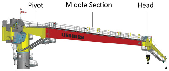
Figure 1.
Box-type boom.
The selection of an appropriate algorithm is rather challenging given the plethora of available optimization algorithms. For the BTB optimization problems, heuristics derived from the manual process, a metaheuristic, and an approach based on a series of linear programs are considered as viable candidates. To select the most suitable algorithm for a problem from a set of candidates, a comparison of the algorithms is required. This is frequently done by using results from empirical comparisons on benchmarks [4,5] since the no-free-lunch theorem [6,7] implies that there is no universal best algorithm. Such benchmarks compare the algorithms based on the obtained solution quality and the necessary computational requirements.
For end-users of such algorithms, however, further criteria which are not considered in such benchmarks are of almost equal importance. Examples of such criteria are the adaptability of the algorithm, required expert knowledge to tune algorithmic parameters or to comprehend the solution creation process, and system integration requirements. Utilizing an analysis tool from quality function deployment (QFD) [8], this paper describes the design of a decision matrix (DM) that allows systematically discussing the strengths and weaknesses of various algorithms. The elements within the developed DM are derived by experts from the fields of optimization and engineering design and incorporate end-user requirements and criteria based on the performance measures used in benchmarks.
The DM applied is tailored to the BTB design task and the considered optimization algorithms. To validate the proposed DM within a proof-of-concept, two scenarios for applying the DM are considered: (1) as a tool for selecting an algorithm before applying the algorithm; and (2) as a performance indicator for a comparison of algorithms applied to a benchmark. The first scenario represents the typical application scenario within the design process since it is rarely feasible to implement all suitable algorithms and make a comparison afterward. The second scenario highlights that the DM can be combined with current benchmarks.
The paper is organized as follows. Section 2 provides an overview of the related work with regard to the QFD method and the algorithm selection problem. In Section 3, the components of the DM are described. Section 4 introduces the BTB design task and its optimization potential. The two optimization problems considered, the algorithms applied, the results obtained, and the evaluations based on the DM are addressed in detail in Section 5 and Section 6. In Section 7, the results of applying the introduced decision matrix as well as the methodology itself is discussed. The paper is concluded in Section 8.
2. Related Work
The related work is divided into two parts: quality function deployment and optimization algorithm selection.
2.1. Quality Function Deployment
Quality function deployment (QFD) is a method that originally aims at ensuring the teleological aspects of product development when the customer needs to drive the product design [9,10]. It is a structured, process-oriented design method that goes back as far as the late 1960s and early 1970s [8]. The major characteristic of QFD is that it is a “people system” [11], i.e., customers and developers/engineers participate together in the product development process. The tools used within the process aim at ensuring the product quality and customer satisfaction. One tool within the QFD process is the “House of Quality” (HoQ) [12], an analysis tool that relates customer requirements and technical properties of a product or a system on different levels of abstraction [11] and enables one to prioritize them [13].
In this work, a specially designed HoQ is applied to the optimization algorithm selection problem to determine the best suitable algorithm given certain customer requirements and preferences. To the best of our knowledge, this is the first time that the HoQ is applied to the optimization algorithm selection problem.
2.2. Optimization Algorithm Selection
The algorithm selection problem was first formalized by Rice [14]: Starting from a set of problems which are represented by certain features, a selection mapping shall be learned to choose the most appropriate algorithm from a set of available algorithms. The most general form of such selection mappings are taxonomies based on certain problem characteristics [15,16]. In the case the problem is explicit convex, the algorithm can be selected from a set of well-established methods such as the simplex algorithm [17], interior point methods [18], or various gradient-based methods [19,20].
In the case the evaluation of a solution requires simulation tools, gradient information might not be available, and the problem characteristics are often (partially) unknown. In such situations, the algorithm is typically selected from the class of direct search methods. This class is loosely defined but contains methods based on model building [21], heuristics and metaheuristics. Heuristics are problem-tailored algorithms and metaheuristics are general purpose optimization algorithms, often imitating natural phenomena [22,23]. The task of selecting the most appropriate algorithm from the class of direct search methods remains a difficult challenge [24].
Naturally, algorithm selection can be based on theoretical and/or empirical knowledge. Theoretical results for direct search methods are scarce [25,26] and comparisons between algorithms often consider only a single function class (see, e.g., [27]). Empirical comparisons between algorithms are much more frequently employed. Here, the algorithms are ranked based on their performance, e.g., towards the automatic recommendation of the most appropriate one for a specific function [28] or over a set of functions, so-called benchmarks. The literature on benchmarks is rich (cf. [29,30,31,32,33,34,35,36,37]), ranging from benchmarks based on mathematical functions to benchmarks based on instances of real-world problems. However, the results obtained from a specific benchmark are not easily generalizable nor transferable to different problems not included in the benchmark.
Next to the problem-dependent performance of the algorithms, the performance is also dependent on the chosen algorithmic parameters, meaning the algorithm selection problem is followed by an algorithm parameter selection problem. For practitioners, this means after an algorithm is selected, determining suitable parameter values (population size, mutation rates, step sizes, etc.) might require a substantial amount of resources (parameter tuning). To overcome this challenge, methods for automatic configuration of algorithmic parameters were developed within the last decade [38,39,40,41].
Not addressed by these benchmark approaches are the preferences and requirements at the algorithm by the end-users. End-users might prefer, for example, an algorithm that can be applied to the whole product range with minimal changes over the best performing algorithm which requires a high effort for integrating the algorithm in the operational system. A major contribution of this work is to present an approach for integrating the end-user requirements into the algorithm selection process.
3. Method
The aim is to compare different optimization algorithms on the same optimization problem by using quantitative criteria of the algorithms as well as qualitative criteria derived from end-user requirements. The results obtained are then not of the common type “algorithm A is x-times faster than algorithm B”, but rather “given end-user requirements C, algorithm A is preferred over algorithm B”.
First, in Section 3.1, the approach on how to build a DM for the algorithm selection problem is presented. Second, the components of the derived DM are presented and described in detail in Section 3.2.
3.1. Methodology—Building a Decision Matrix
An HoQ chart consists of criteria in two dimensions and the relationships between the criteria across and within the dimensions. In the proposed DM, an adapted variant of an HoQ chart, the dimensions are demanded quality (the end-user requirements) and quality characteristics (the behaviors/properties of the optimization algorithms). Building the DM requires experts from the respective field(s) for defining the criteria and their relationships. In our case, two algorithm developers and two experts from the field of engineering design were involved. In several discussions and by using data from interviews conducted with end-users from the area of engineering design, the criteria and their relationships were iteratively developed. The final DM, especially the relations between the criteria, represents the consensus view of all experts involved.
In traditional QFD, the analysis of competitive products is done using an absolute rating, e.g., between 0 and 5, on the demanded quality criteria. These ratings do not take into account the various relations of a single demanded quality criterion to the quality characteristics and their relative weights. Thus, these absolute scores do not reflect the importance with regard to the quality characteristics (i.e., two criteria can be rated the same, even though one criterion has much stronger relations to the end-user requirements). We therefore introduce a score weighting the absolute rating of the demanded quality criteria with the correlations and relative weights of the quality characteristics:
In Equation (1), is the absolute rating of the ith demanded quality criterion, is the numerical value corresponding to the strength of the relationship between the ith demanded quality criterion and the jth quality characteristic (9 for strong, 3 for moderate, 1 for weak, and 0 for no relationship), and is the relative weight of the jth quality characteristic. These scores for the demanded quality criteria are visualized using a bar diagram. The total score of an algorithm is the sum over all scores . The developed DM with all criteria, their relations, values for two algorithms, and the bar diagram is shown in Figure 2.
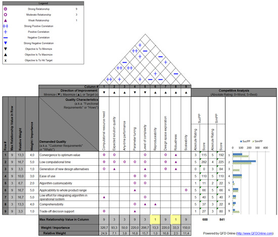
Figure 2.
Design optimization decision matrix template.
The user input for a given DM is to define an absolute rating, , for an algorithm for each demanded quality criterion and to define the importance, i.e., the values in the column “Weight/Importance”, for all demanded quality criteria . The relative weight of the quality characteristics, in Equation (1), depends on through
where is the relative weight for the kth demanded quality criterion.
3.2. Resulting Decision Matrix for Algorithm Selection
In the following, the considered individual criteria are briefly defined. For brevity, the correlations between the quality characteristics (Table A1 and Table A2), and the relationships across the dimensions (Table A3 and Table A4) can be found in the Appendix A.
3.2.1. Demanded Quality Criteria
The demanded quality criteria are end-user requirements on the optimization algorithms. Their importance, which can vary for different end-users or different optimization problems, can be defined in the column “Weight/Importance” on a scale from 0 (not important) to 5 (very important). Each algorithm can be ranked in the “Absolute Rating” column for each criterion, again on a scale from 0 (does not fulfill criterion) to 5 (completely fulfills criterion).
- Convergence to optimum value: The capability to always converge towards near-optimal solutions.
- Low computational time: The capability to find high quality solutions in a for the end-user acceptable time.
- Generation of new design alternatives: The capability to generate distinct design alternatives other than those obtained by small variations of the initial product configuration.
- Ease of use: The effort required to set up the algorithm for the problem. This includes, among others, the selection process for the algorithmic parameter values and how the user can interact with the algorithm.
- Algorithm customization: The possibility and the effort required to make significant changes to the algorithm to increase the application range or to change parts of the algorithm.
- Applicability to whole product range: The effort required to apply the algorithm to the whole product range, e.g., lower/higher dimensional variants of the same problem or problems with slightly changed constraints.
- Low effort for integrating algorithm in operational system: The effort required to implement the algorithm into the system and to set up connections with the required external tools, e.g., CAD and CAE systems, databases, computing resources, and software libraries.
- Comprehensibility: The level of expert knowledge required to understand the solution creation process and the solution representation.
- Trade-off decision support: The capability to investigate different objectives and different constraint values with the same or a slightly modified algorithm.
3.2.2. Quality Characteristics Criteria
The quality characteristics comprise several properties of an algorithm. For each criterion, a direction of improvement is provided (see row “Direction of Improvement” in Figure 2).
- Computational resource need: The computational resources, e.g., number of function evaluations or run times, required to obtain a high-quality solution. One aims at minimizing the need for computational resources.
- Expected solution quality: The expected quality of the solution obtained. Solution quality is directly related to the objective function value and the constraint satisfaction. It is to be maximized, regardless of whether the objective function is minimized or maximized.
- Any-time performance: The ability of an algorithm to provide a solution at any-time and to continuously improve this solution by using more resources. In an ideal situation, the solution improvement and the increase in resources exhibit a linear relationship. The aim is to maximize any-time performance.
- Parameter tuning: A combination of the required computational resources and expert knowledge to select well-performing values for the algorithmic parameters. The direction of improvement for parameter tuning is to minimize it.
- Level of complexity: The increase in complexity of an algorithm compared with Random Search. Complexity is increased by using special operators or methods for the solution generation, but also by using surrogates or parallel and distributed computing approaches. The complexity increase should result in finding better solutions and/or getting solutions of the same quality in less time. The aim is to minimize the level of complexity.
- Reproducibility: The capability of an algorithm to provide the same, or close to, solution by rerunning the algorithm with the same setup. Reproducibility is to be maximized.
- Design space exploration: The capability of an algorithm to create and evaluate vastly different solutions within the feasible design space. A maximum of design space exploration is preferred.
- Robustness: The capability to provide solutions which exhibit only small changes in their quality when the problem itself undergoes small changes. Robustness is to be maximized.
- Scalability: The capability to obtain high-quality solutions on problems with increased dimensionality within an acceptable time and with at most changing the values for the algorithmic parameters at the same time. The aim is to maximize scalability.
3.3. General Remarks on Criteria, Correlations, and Relationships
The selected criteria aim at representing the most important characteristics in each dimension with as few as possible criteria. Thus, the DM could be extended in each dimension by adding other criteria or by splitting an existing criterion, e.g., “Level of complexity” into “Use of surrogates”, “Use of parallel resources” and “Algorithm complexity”.
Next to defining the criteria, selecting the strengths for the correlations and relationships involved several rounds of discussions. In the end, strong correlations and relationships were applied to known and mostly deterministic effects, such as the increase in computational resources if the expected solution quality should be improved or a high effort for parameter tuning is required. Anything that happens frequently, but might be strongly dependent on the algorithm or the problem instance was regarded as a medium relationship or as a positive/negative correlation. For example, increasing the design space exploration does affect the convergence towards the optimum, but the relationship is not that obvious (no convergence would be observed for extreme levels of exploration). For all other relationships where a dependence could not be excluded, a weak relationship was selected.
We need to emphasize that the presented DM, including the correlations and relationships, is subjective due to the experts involved. Hence, the DM should not be considered as fixed, but rather as a template that should be adapted for different optimization problems or could be refined for meeting specific needs.
4. Box-Type Boom Design and Optimization
BTBs as engineered at LWN are typical Engineer-to-Order products since they have to be re-designed for every offer due to changing geometrical and structural requirements. As indicated in Figure 1, a BTB consists of the pivot and head part as well as the middle section. The pivot and head components are selected from a list of standardized parts, leaving the middle section as the design task. Typically, the pivot component is larger than the head component such that the middle piece gets narrower towards the head section.
4.1. BTB Design Task
The middle section is a hull consisting of welded together metal sheets at the outside, and stiffeners and bulkheads at the inside. Its design depends on various factors, such as the dimensions of the pivot and head components, the length of the boom, and the load cases (and therefore the structural parameters). As Figure 3 shows, the middle section of the boom is divided into segments, each of which lies between two bulkheads or a bulkhead and the pivot or head part. The bulkheads are placed at equal distances, starting from the pivot to the head end, resulting in equally long segments for the first to the second last segment. The length of the last segment is determined such that the total length of the middle section is reached.
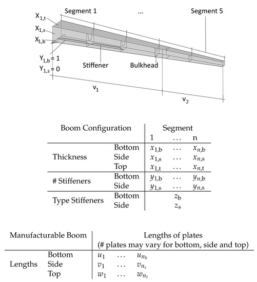
Figure 3.
Box-type boom design: Variables of a boom configuration and of a manufacturable boom (adapted from Fleck et al. [3]).
Following the description and notation of Fleck et al. [3], each segment is specified by five variables: thicknesses of the bottom, side (same for both sides), and top of a segment as well as the number of stiffeners on the bottom and side of a segment. Furthermore, there are two global variables, the type of stiffeners on the bottom and the side of the segments. A boom configuration is defined to be one specific setting of these variables (see Figure 3). The variables of a boom configuration have to be chosen such that the structural requirements are fulfilled (i.e., the boom can carry the defined load cases).
The final, manufacturable middle section consists of metal plates spanning several segments, which are welded together in appropriate places (e.g., with a large enough offset between any two welding seams) to form the hull of the boom. The variables to define the manufacturable boom are given in Figure 3. The thickness of each plate is specified to be the thickness of the thickest segments among the segments it spans. The five-segment boom example in Figure 3 has welding seams in the second last segment, indicated by the black lines on the bottom, side, and top in this segment. Thus, the bottom, side, and top, respectively, are each split into two plates (i.e., ) with lengths and (bottom), and (side, as indicated in the figure), and and (top).
4.2. Optimization Potential of the Box-Type Boom Design
As a manual process, the engineering design of a BTB and the generation of production-ready documentation can take up to 80 h. For the automation of the design of a BTB, a Knowledge-Based-Engineering (KBE) application has been developed together with LWN. For details, the readers are referred to the work in [2]. From this KBE-application, two tasks with high optimization potential were identified. These two problems are:
- Boom Configuration: The structural analysis defines the metal sheet thicknesses as well as the number and type of stiffeners in each segment (boom configuration), to define a BTB that can safely lift certain load cases at a given length. Currently, these parameters are determined by the engineer, through experience and a trial-and-error strategy, and evaluated using a structural analysis tool.
- Plate Partitioning: An appropriate partitioning of the hull of the BTB into single plates is required to be able to manufacture the boom. Initially, this task was performed manually by the design engineer, and later, in the course of the implementation of the KBE-application, replaced by a heuristic approach (termed Successive Plate Partitioning) [42].
Typically, both the structural analysis and the plate partitioning have to be carried out anew for every ordered boom, since the boom length and load cases are customer-specific. Furthermore, both are cumbersome tasks with a rather large solution space. Thus, they both bear the potential to be further automated and optimized.
Following this identification of the optimization potential, the optimization of the BTB design (cf. Figure 4) is carried out accordingly in two steps: (1) Boom Configuration Optimization (see Section 5); and (2) Plate Partitioning Optimization (see Section 6). The mathematical formulation of the optimization problems are given in the respective sections.
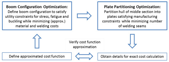
Figure 4.
Steps of the Box-Type Boom optimization.
As depicted in Figure 4, the boom configuration optimization uses an approximation of the cost function (lower left corner in the figure), since the exact costs can only be calculated once all manufacturing details are known. This, in turn, is only the case after performing the plate partitioning optimization of Step 2 (lower right corner). Thus, a comparison of the approximated cost function and the exact cost function has to be carried out to verify the accuracy of the approximation.
According to Ravindran et al. [33], it can be “fruitful to consider [...] sequential optimization using a series of sub-problems or two-level approaches in which intermediate approximate models are employed”. We here select this two-step procedure due to the distinct nature of these two optimization problems and the benefit of significantly less computational costs when using the approximate cost function. However, it may be possible that the global optimal solution may not be found.
5. Boom Configuration Optimization
5.1. Problem Definition
The optimization problem was introduced by Fleck et al. [3] as a constrained single objective optimization problem. Following their description, the objective is to find a boom configuration that minimizes material and welding costs for the plates and stiffeners while satisfying the structural and some other constraints (see below). Collecting the variables of a boom configuration in , and , the objective function is defined as
with
| material costs of the metal depending on the thickness ; | |
| material costs of the stiffener depending on the stiffener type ; | |
| welding costs of the stiffener depending on the stiffener type ; and | |
| welding costs of the plates depending on all thicknesses . |
While the material and welding costs of the stiffeners can be calculated independently for each segment, the welding costs of the boom depends on all thicknesses, since the metal sheets of the segments can be combined to larger plates. This may also affect the material costs of the metal sheets, in the case segments with different thicknesses would be combined to a single plate (typically then using the thicker one).
Since, at this stage, the exact costs are not yet available, a cost approximation is used (and verified in Section 5.3 against the true cost function). To approximate the welding costs of the plates, a welding seam is calculated if
- two consecutive segments have different metal thicknesses; or
- two consecutive segments have the same metal thicknesses and the previous three segments were already combined (i.e., were also of the same thickness).
This approximation assumes that up to three segments can be combined into a long plate (based on metal plate size restrictions) and that the welding seams are exactly placed at the end of a segment. On the one hand, the placement of the welding seams in this way is in practice not allowed due to manufacturability constraints (no two welding seams are closer by than a certain offset), but, on the other hand, allows us to calculate the material costs of the metal sheet independently for each segment.
Besides defining the cost function, the optimization problem also contains a set of constraints, which ensure that the designed boom configuration yields a functioning crane. These constraints are formally defined within the optimization problem below and elaborated thereafter (following Fleck et al. [3]).
subject to
.
The first set of constraints (Equations (5)–(7)) ensures that the utility constraints with respect to stress (denoted by ) and fatigue () on the bottom, side, and top as well as with respect to buckling () on the bottom and side are fulfilled for each segment. Any value larger than 1 is a violation, and, the larger the value, the higher is the violation. A structural analysis tool is used to calculate the utilizations for a given boom configuration. In the second set of constraints (Equations (8)–(10)), the allowed thicknesses for the plates on the bottom, side, and top, respectively, are defined. Equation (11) states that these thicknesses are non-increasing from the pivot part to the head part. The number of stiffeners is limited to lie between 0 and 3 (bottom), and 0 and 2 (side) (Equations (12) and (13)), and is non-increasing from the pivot part to the head part (Equation (14)). Finally, the four allowed types of stiffeners are indicated in Equation (15).
5.2. Optimization Approaches
The problem is described by discrete variables with both linear and non-linear constraints. The problem can be considered as “oracle-based” or “black-box”, since a structural analysis tool is used for the constraint evaluation. As shown in [3], total enumeration is not feasible. Thus, we first describe a heuristic approach using as little evaluations with the structural analysis tool as possible, to quickly reach a (near) optimal solution. This approach is explained in Section 5.2.1.
We also apply a metaheuristic approach, in particular, an Evolution Strategy (ES) [43,44]. However, since such algorithms typically require 10,000 or more solution candidates, this is not directly feasible. Therefore, we apply surrogate modeling to replace the computationally expensive structural analysis tool. Earlier research showed that the structural analysis tool can indeed be approximated well with surrogate models [3]. This surrogate-assisted optimization approach is described in Section 5.2.2.
5.2.1. Heuristic Optimization Approach
We here describe the developed heuristic optimization procedure for achieving a (near) optimal boom configuration. This is pursued in a three-step manner, as illustrated in Figure 5.
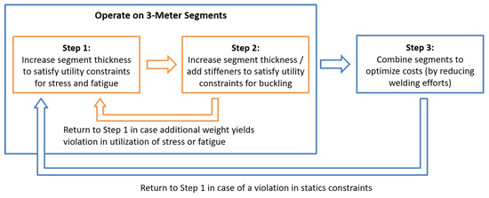
Figure 5.
Three-step heuristic optimization approach.
In Step 1, only stress and fatigue are considered, buckling is considered separately in Step 2. This separation is possible since stress and fatigue only rely on the metal thicknesses, but not the stiffeners. For buckling, both thicknesses and stiffeners have to be taken into account.
The first two steps operate solely on the segments: In these steps, the segments are considered to be completely independent of each other. In the case of a violation in the structural utility constraints, this independence assumption enables the enumeration of all of the more stable (i.e., thicker and/or more stiffeners) bottom/side/top segment configurations separately and to order them by segment costs to select for each bottom, side, and top the next cheapest segment configuration to update the boom configuration. Only in the third step the costs are optimized also including the welding costs of the boom (i.e., only here the complete objective function of Equation (4) is used).
We next describe of each of the three steps. Note that the constraints in Equations (8) to (10) as well as in Equations (12) and (13), defining the admissible values of the plate thicknesses and the number of stiffeners, are fulfilled at any time, since the values are chosen in accordance with these sets.
(1). Fulfilling utility of stress and fatigue (constraints in Equations (5) and (6))
The optimization starts with an initial boom configuration, typically the cheapest possible one, i.e., no stiffeners and minimum plate thicknesses for each segment. The configuration is evaluated using the structural analysis tool. If the utilization of stress or fatigue is greater than one on the bottom, side or top of any segment, the respective segment configuration (and with it the boom configuration) is adapted by increasing the corresponding thickness to the next higher value. Whenever the number of stiffeners is larger than zero, it is set back to zero. The resulting boom configuration is then tested with the structural analysis tool. This process is repeated until no violations in the constraints of stress and fatigue are found, such that the procedure can continue with Step 2.
In this step, no explicit cost evaluation is needed, since the thicknesses are only changed to the next higher value, which naturally is the next cheapest option. Note, however, that it might be possible that not all violated constraints of stress and fatigue would be necessary to be adapted simultaneously. It could be possible that it had been enough, e.g., to increase the value of one segment and reach no violation also for the consecutive segment, or to increase only certain values on the bottom and top and reach no violation on the sides. This, however, would yield an explosion of possibilities and thus of run time. Thus, in the heuristic, these values are increased simultaneously for all bottom, side, and top segments, where a violation occurred. This comes at a cost: the global optimum might be missed.
(2). Fulfilling utility of buckling (constraint in Equation (7))
The second step is divided into two sub-steps.
- (a)
- Taking constraints of Equations (11) and (14) into accountConsidering the boom configuration output of Step 1, if there are any violations in the utilization of buckling, or non-increasing plate thicknesses or the number of stiffeners, the boom configuration is updated as follows. For each segment (i.e., starting from the segment closest to the head end), it is verified whether the thickness and/or the number of stiffeners of bottom, side or top is higher than the previous segment i. If so, the respective thickness and/or the number of stiffeners of segment is set to that value of segment i. If any changes were made, the updated configuration is stored as the first suggestion for the next boom configuration to be evaluated. Then, all possible combinations of more stable segments for the bottom and side, respectively, are generated and if the generated version is cheaper than the currently defined next configuration, the latter is replaced with the cheaper one. This is done to trade-off segment thickness and the number of stiffeners with regard to costs. Once the update is made for each segment at the bottom, side, and top, the boom configuration is evaluated with the structural analysis tool. This procedure is repeated until all buckling constraints as well as the constraints in Equations (11) and (14) are fulfilled. Afterward, the utilizations of stress and fatigue are checked again. If there are any violations, the procedure returns to Step 1, otherwise, it continues with Step 2b. In addition, in this step, it might be possible, due to the simultaneous changes, that the global optimum is missed out. However, similar to the argument in Step 1, the simultaneous changes are required to avoid run-time explosions.
- (b)
- Taking constraints of Equation (15) into accountRecall that, thus far, due to the independent consideration of all segments, each segment could have different stiffener types. This is corrected now to fulfill the constraints of the same type of stiffeners for all bottom segments and all side segments. First, the currently used types on the bottom and side, respectively, are extracted from the segment configurations. Restricting the types of stiffeners to the already used ones, all more stable configurations are generated (one at a time for bottom and side, respectively). For each of these boom configurations, the utilizations of stress, fatigue, and buckling are calculated and, if all statics constraints are fulfilled, the costs are calculated. The cheapest of these configurations is used. If none of these configurations fulfills all statics constraints, the procedure returns to Step 1; otherwise, it continues with Step 3.
(3). Optimizing for costs
In the third step, thicknesses of segments are modified to minimize costs with regards to welding and material according to the objective function in Equation (4).
To reduce the welding costs, starting from the base configuration handed over from Step 2b, the bottom/side/top segment thicknesses are successively and recursively increased, if possible, starting from the second segment, in order to be able to potentially save welding seams when combining segments to larger plates (in our case, combining up to three segments of the same thicknesses).
First, for each bottom segment, starting from the second segment, it is checked whether the segment thicknesses can be increased to the next, the second next or third next higher thickness while keeping side and top segment configurations constant. Any resulting valid configuration is stored and additionally considered as starting configuration when looking at the following segments. In this way, first, variants of the bottom configuration are generated and the cheapest among those is taken, and similarly for the side and top segments. These three solutions are combined to form the cost-minimized boom and again evaluated with the structural analysis tool. If there is a violation in the structural utility constraints, the procedure returns to Step 1; otherwise, it terminates and outputs the final Boom Configuration.
5.2.2. Metaheuristic Optimization Approach
The second approach to solve the boom configuration optimization problem utilizes an Evolution Strategy, a metaheuristic. To be able to apply these kinds of methods to the boom configuration optimization, two issues have to be dealt with:
- Convert the constrained optimization problem into an unconstrained one.
- Overcome run time issues due to expensive evaluations of the structural constraints by using surrogate-assisted optimization.
Unconstrained Optimization Problem
Since metaheuristic algorithms often do not handle constraints explicitly, they have to either be incorporated in the objective function, e.g., by using penalty functions [45], or be addressed in the encoding of the variables, e.g., by allowing only valid solutions regarding those constraints, yielding an unconstrained optimization problem.
For the BTB optimization problem, a penalty for the constraints in Equations (5)–(7) is designed and added to the objective function. The new objective function is
with r as constant penalty factor which has to be set in the optimization algorithm. By defining the penalty functions as the maximum of zero and the constraint, e.g., , it is ensured that only for invalid solutions a penalty is added.
The other constraints are taken care of in the solution encoding. Towards this end, we use an integer-vector of length , containing all the variables of the boom configuration. By only selecting values from the given sets of thicknesses as well as number and type of stiffeners, it is ensured that the constraints in Equations (8)–(10), (12), (13) and (15) are fulfilled. To ensure that the constraints in Equations (11) and (14) are not violated, the thicknesses and the number of stiffeners are sorted in descending order from the pivot- to the head-end.
We opt for an Evolution Strategy (ES), mainly because ES is traditionally specialized on fix-length vectors. Because we use an integer-vector, the values of the vector after manipulation are rounded to the next feasible integer.
Run-Time Reduction By Surrogate-Assisted Optimization
One common technique to reduce the computation time is surrogate modeling [46,47] or, in the case of optimization, surrogate-assisted optimization [48]. The main idea is to replace the original, expensive evaluation (Equation (16)) with a simple model . To create surrogate models, machine learning techniques [49] are used. These methods use data of previously performed expensive evaluations as input to learn a model that estimates the objective value of unseen evaluations. The obtained models are not as precise as the simulation model but can be evaluated fast and are accurate enough to guide the optimization algorithm to promising designs. However, the final results must be verified with the expensive evaluation in case the optimization was misled with an improper surrogate model.
In general, there are two ways of applying surrogate models with optimization. First, in offline or sequential modeling [50], a single surrogate model is obtained before the actual optimization and not changed during the optimization. Second, in online or adaptive modeling, modeling is also performed during the optimization to adapt the model during the search process. In this work, we used an offline model for optimizing the boom configuration.
To train the surrogate model, we sampled the search space and evaluated the samples with the structural analysis tool to obtain reference data. Using only random samples would mean that only solution candidates with a low quality would be included since good solutions are unlikely to be found with random sampling. Therefore, we also included samples obtained from weakly converging evolution strategies. In total, 500 samples (250 random and 250 from ES) were used. For more detailed information on the sampling and data generation, we refer to the work in [3].
In this work, we used Random Forests [51] because they were considerably easier to apply than white-box models based on symbolic regression [3,52]. After the modeling phase, we obtained a model for each of the structural constraints (three stress, three fatigue, and two buckling). Only after the optimization, we performed a validation step by evaluating the best solution per generation with the actual structural analysis tool.
5.3. Results
5.3.1. Cost Function Comparison
For the boom configuration optimization, an approximation of the exact cost function will be used due to run time reasons, as mentioned in Section 5. The approximation only concerns the material and welding costs of the metal sheets and not the stiffeners.
For the comparison of the approximated and real cost functions, the number of segments was chosen to lie between 4 and 23 (yielding lengths of the middle sections between 9001 mm and 69,000 mm). For each number of segments, 2000 valid boom configurations were randomly generated and the exact and approximated costs were calculated. The results are shown in Figure 6.

Figure 6.
Comparison of cost approximations for metal sheets; the colors indicate the number of segments, starting at the bottom left with 4 segments (dark blue) to the top right with 23 segments (yellow).
Overall, the approximated cost function underestimates the exact costs slightly, however, it yields very good results in terms of ordering the solutions. The same holds when looking at the material and welding costs separately, see the respective graphs in the Supplementary Materials.
The reason for the underestimated costs is two-fold. On the one hand, the material cost is underestimated since for the true cost function the segments are collected to longer plates also if they are of different thicknesses, and the final plates have the thickness of the thickest segment they span. This also leads to a certain underestimation of the welding costs, since seams of thicker plates are more expensive than of thinner plates. On the other hand, the welding costs of the true cost function include additional factors for testing certain seams using ultrasonic and magnetic particle inspections, which are not included in the approximated cost function.
5.3.2. Optimization Comparison
An overview of the results on the five test cases is given in Table 1. The reference solutions (Ref. columns in Table 1) represent real manufactured booms without using any optimization.

Table 1.
Results of the boom configuration optimization.
Comparing the reference solution and the solution of the heuristic approach, the value of the objective function is lower in all test cases when using the heuristic optimization. These cost savings can be achieved through using the utilizations better, i.e., in most cases obtaining higher, yet still valid degrees of utilizations. An exception is Test Case 1, where the average utilization for buckling of the reference solution is very close to one, due to an unbalanced selection of plate thicknesses. By choosing better values, both costs and utilization degrees can be improved.
The applied ES is a (20 + 100)-ES, which was run for 100 generations and 10 repetitions were performed. Further improvements with the ES (including surrogate modeling) requires a significantly higher amount of calls to the structural analysis tool. The number of calls shown in Table 1 (see column Analysis Tool Calls) lists the calls necessary for training the surrogate models (500 samples) and the calls that were performed during the validation of the results. The number of validation-calls is varying due to caching effects since we do not evaluate the same boom twice. Note that, for both ES and heuristic, the run time is dominated by the run time of the structural analysis tool.
5.3.3. Decision Matrix for Boom Configuration Optimization
In Figure 7, the DM for both algorithms, before and after the analysis of the obtained results, are given. Before optimization, the ES was expected to perform better in part due to the ability to generate design alternatives and better convergence behavior. After the optimization, it showed that the heuristic had a better than expected performance in “Convergence to optimum value” and the ES was worse than expected in “Low Computational Time”, yielding a reversal of the algorithms ranking. In addition, for the ES the use of Random Forest led to an improvement with respect to “Ease of Use” and “Algorithm customization”, but the respective models can no longer be interpreted. Hence, “Comprehensibility” is lowered. The complete DM for both cases are provided in the Supplementary Material. The given DM is the consensus view of three experts.
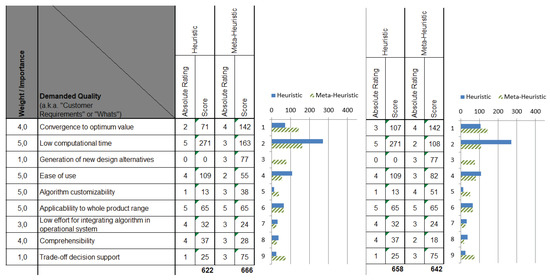
Figure 7.
Decision Matrix for Boom Configuration before optimization ((left) with Demanded Quality Criteria) and after optimization (right). Note that, for a better representation, only the scoring for comparing the algorithms are shown.
6. Plate Partitioning Optimization
6.1. Problem Definition
The second step of the BTB optimization addresses the plate partitioning (see Figure 4). The objective of this optimization problem is to minimize the number of welding seams along the boom while fulfilling a set of constraints, mostly concerning manufacturability. The underlying motivation is that for every additional plate, an additional welding seam has to be made, which increases the costs since welding seams are typically more expensive than material. Fewer welding seams means fewer plates (i.e., better usage of metal sheets) and fewer steps within the manufacturing of the boom. However, these two points are not reflected in the cost function (Equation (4)).
Recalling the parameter definitions in Section 4, the plate partitioning optimization problem is formalized as
subject to
and equivalently for side plates and top plates .
The constraint in Equations (18) and (19) define the minimum and maximum length of the bottom plates, respectively (the latter one is shown in Figure 8). Equation (20) states that the lengths of all single bottom plates have to sum up to the total length of the middle section (denoted as , see also Figure 8). In Equation (21), it is described that no welding seam of the bottom plates is within to any of the bulkheads. An example of this is shown in Figure 8 for the two side plates and the third bulkhead. Finally, Equation (22) states that no welding seam of two bottom plates is within to any welding seam of two side plates (see again Figure 8 for an example).
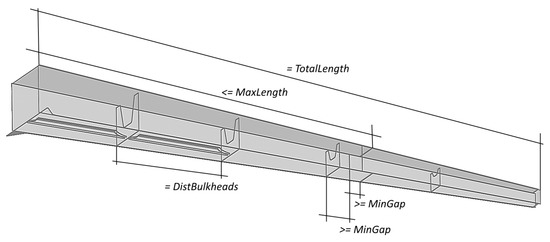
Figure 8.
Middle piece of a BTB with indicated variables and constraints for the plate partitioning.
For the side plates, a set of similar constraints has to be defined. The equivalent of Equation (22), however, includes the variables of the side and top plates, ensuring that no seam of any two side plates lies within of any seam of two top plates. The constraints for the top plates only have to be defined equivalently to Equations (18)–(20); Equation (21) is not necessary since the bulkheads are only welded to the bottom and side plates and not to the top plates, and Equation (22) is not needed since this is already covered by the constraints of the side plates.
Finally, we want to note that some further details (e.g., the taper of the boom or a welding gap between any two plates) were neglected from the formulation for clarity.
6.2. Optimization Approaches
In the deployed KBE-application [2], the plate partitioning is performed using a heuristic optimization approach, which we refer to as Successive Plate Partitioning (SucPP). This procedure, even though already in use, is described in detail for the first time in this paper (Section 6.2.1). A second developed approach based on a series of Linear Programs (LPs) [17] is presented. This second approach, referred to as Simultaneous Plate Partitioning (SimPP), is outlined in Section 6.2.2.
6.2.1. Successive Plate Partitioning
The idea of SucPP follows the routine which the design engineer used to determine the plate partitioning manually. The calculation of the plate lengths is achieved in an incremental, three-step manner.
- Determine the lengths of the top plates: Since no other lengths are set yet and the bulkheads are not welded to the top plates, the length of each top plate is chosen as long as possible, i.e., is set to , or, in the case of the last plate, is determined such that the sum of all plates is equal to , the length of the middle section.
- Determine the lengths of the bottom plates: The lengths of the bottom plates are restricted by the positions of the bulkheads. Since the lengths of the side plates are not determined yet, these constraints can be neglected at this point. Thus, the length of each bottom plate is determined to be as long as possible, yet avoiding conflicts with the bulkheads. In particular, if the gap between the welding seam of two bottom plates and the welding seam of a bottom plate and a bulkhead would be smaller than , the bottom plate is shortened to an appropriate length. As for the top plates, the last bottom plate is assigned the appropriate length to reach .
- Determine lengths of side plates: All determined parts have to be taken into account, meaning that the length of each side plate is restricted by the lengths of the top and bottom plates, as well as the position of the bulkheads. As in Point 2, if any two welding seams are too close to each other, the side plate is shortened to an appropriate length. As above, the length of the last side plate is chosen to reach .
This strategy for calculating the lengths of the single plates has the advantage of being transparent and comprehensible. However, once the length of a plate is determined, it cannot be changed, even if it were advantageous for the determination of other lengths.
SucPP does not use the information of the optimized boom configuration. Instead, this information is only used afterward to determine the thicknesses of the resulting plates as the thickest one among the segments that the plate spans.
6.2.2. Simultaneous Plate Partitioning
For the task at hand, the simplex algorithm [17] is a suitable choice since the optimization problem can be re-written as a series of linear programs (LPs). The problem of optimizing the plate partitioning in the sense of achieving the longest plates possible (i.e., smallest number of plates possible) is encoded into a series of LPs. This is needed since the constraints in Equations (21) and (22) are not linear. We demonstrate with an example how this linearization and problem formulation is made using a series of LPs; the general formulation follows analogously.
Assuming a length of the middle section of = 25,000 mm and a maximum plate length 10,000 mm an LP is set up as follows.
The Decision Variables
Informally speaking, to determine the number of bottom (), side (), and top () plates (and thus the number of variables), the total length of the middle section (25,000 mm) is divided by the maximum length of each plate (10,000 mm), and the ceiling of this number is taken as the result. If the simplex algorithm does not find a solution with this number of plates, it is successively increased first for the side, then for the bottom, and finally for the top plates. In our example, this means that there are three bottom (), three side (), and three top plates (), i.e., nine variables in total. Note that the left and right side of the boom are identical.
The Objective Function
Since there are nine variables, the constant weights have to be specified. The objective function is chosen such that the first to the second last plates on the bottom, side, and top, respectively, are made as long as possible (assigning equal weights ). The length of the last plate is merely used to reach the correct total length (setting the corresponding weights ). This means that the function is to be maximized.
The Constraints
The requirements of obtaining the appropriate length for the boom, obeying manufacturing restrictions (minimal and maximal lengths of the plates), and taking the welding seams into account are formalized as follows. If not stated otherwise, the indices and k range from 1 to 3.
- Considering minimum gap between welding seams between plates and bulkheads (corresponding to Equation (21)), as mentioned in Section 4, the bulkheads are positioned at equal distances, starting from the pivot section. To be able to formulate the optimization problem as a linear one, in each LP, only the position of one bulkhead for the first to second last bottom plate can be considered at a time. Thus, a series of LPs is considered, differing in the selection of the bulkheads, among which the best solution is chosen. As an example, assume that, for the current formulation, the third and seventh bulkheads are selected. The constraints are set up such that the first and second bottom plate end between the third and fourth, and seventh and eighth bulkheads, respectively:The formulation for the welding seams between the side plates and the bulkheads is similar.
- Considering minimum gap between welding seams (corresponding to Equation (22)), since all plates have the same restrictions on the length, the constraints of the welding seams between the bottom and side plates can be restricted, such that the welding seams of the first and second bottom plates to the welding seams of the first and second side plates differ in at least . This holds similarly for the welding seams between the second and third bottom and side plates. Thus, we define the following constraints:A similar formulation is made for the side and top plates.
Given the solution of the above series of LPs, the minimum number of plates is determined. However, the solution thus far does not take the segment thicknesses of Step 1 into account. Thus, a second series of LPs can be set up, determining the positions of the bulkheads in the constraints in such a way that the welding seams are set at the borders of the thicknesses of the segments, however, not using more plates than in the first set of LPs. This may lead to a better solution (compared with the real cost function), but potentially be an unsolvable LP. In this case, simply the solution of the first series of LPs is taken.
As opposed to SucPP, SimPP determines the lengths of the plates simultaneously, i.e., there is a trade-off between shortening certain plates to obtain longer plates elsewhere. However, to an engineer the use of such an optimization algorithm may seem like a black box, making it harder to reproduce and verify the result.
6.3. Results
The two optimization approaches are compared to elaborate how much improvement can be achieved by using a mathematical optimization (SimPP) over a heuristic optimization (SucPP). We created BTBs for lengths between and with an increment of . For a fair comparison of the two approaches, we restrict SimPP to determine the longest plates possible (i.e., not taking into account any segment thicknesses). The main results are shown in Figure 9.
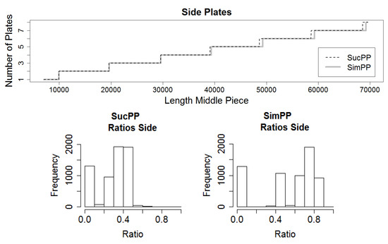
Figure 9.
Comparison of the two approaches for calculating the side plate partitioning.
In the top of Figure 9, the resulting number of plates for the side of the middle section are shown for SucPP (black dashed lines) and SimPP (gray solid lines). As one can observe, SimPP slightly outperforms SucPP for longer booms (length ). For the number of top and bottom plates, the differences in the number of plates are fewer. The respective plots are in the Supplementary Materials.
While in terms of the number of plates the performance of the two approaches is rather similar, SimPP outperforms SucPP in terms of finding longer plate lengths, as shown in the histograms at the bottom of Figure 9. For each of the generated BTBs, the ratio of plate lengths among the first to second last plate lying within 1% of is determined (the last plate is disregarded since its length is merely set to reach the total length of the middle section ). Each histogram shows the frequencies of these ratios over all generated booms for the side plates. The respective histograms for the bottom and the top plates are in the Supplementary Materials. Additionally, in Table 2, some examples for the obtained lengths of the side plates for both approaches are shown.
Table 2.
Examples of resulting lengths of side plates, with . Bold values indicate plates whose length is within 1% of .
From these results, the advantages of using an optimization algorithm become apparent: Instead of setting the length successively as in SucPP (first top, then bottom, and finally side plate lengths), SimPP simultaneously searches for appropriate lengths, leading to a globally optimal solution. For example, in some cases, it is advantageous to shorten a bottom plate (while keeping the same number of plates) in order to obtain longer side plates, which lies outside the solution space of SuccPP.
When comparing SucPP and SimPP using the cost function of Equation (4), we can see in Figure 10 that the costs measured by this function are rather similar for the BTBs inferred by SucPP and SimPP. While this cost-saving with SimPP is marginal, there are other places where costs can be saved, as mentioned in Section 6.1.
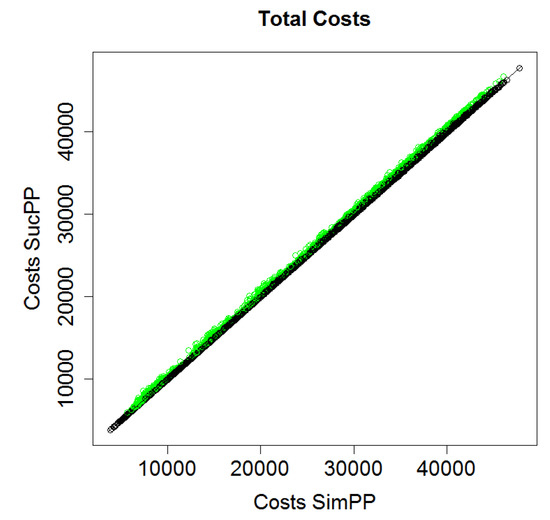
Figure 10.
Cost comparison of SucPP and SimPP; the green circles indicate booms with a cost saving of 1% or more by using SimPP.
Regarding the time requirements of SucPP and SimPP, the run times are compared by measuring wall-clock time. The results are presented in Figure 11 as a box-plot, showing the time requirement in seconds in dependence of the boom length.

Figure 11.
Time Comparison of: SucPP (left); and SimPP (right).
For both algorithms time requirements increase, when additional plates are introduced. However, even for SimPP and long booms, the run time stays under 5 s, which is completely acceptable for an industrial application. The decrease in computation time for certain lengths of the middle section in SimPP, especially at 49, 59 and 69 m, can be explained by the fact that for these lengths there are only very few (potentially only 1) possible solutions for setting up and subsequently solving the LP with the given number of plates.
Decision Matrix for Plate Partitioning
In Figure 12, the DMs for SimPP and SucPP before and after having the information on the achieved results are presented. In both stages, SimPP was the preferred algorithm. SucPP provided better than expected solutions in an acceptable time, while SimPP did not need large amounts of computational resources and can be applied to the whole product range (the product range covers booms up to 70 m). Both algorithms are easier to use than expected. The DMs shown represent the consensus of three experts. The complete DMs can be found in the Supplementary Materials.
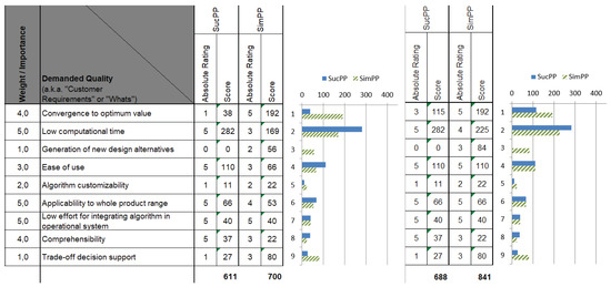
Figure 12.
Decision Matrix for Boom Configuration before optimization ((left), with Demanded Quality Criteria) and after optimization (right). Note that, for a better representation, only the scoring for comparing the algorithms are shown.
7. Discussion
7.1. Algorithm Selection
Using a DM for comparing algorithms allows incorporating the end-user requirements/preferences into the comparison. This adds another dimension to algorithm comparisons, which are usually based solely on the performance on some benchmark, and aids the decision process for selecting the “right” algorithm. By using a tool from QFD, the algorithm selection is based on a systematic framework. The drawback of the method is that it inserts a set of subjective values into the comparison.
Two steps are required for building a DM: (1) defining the criteria for the two dimensions; and (2) finding the relationships between the criteria. While the examples in this work and some of the experts involved come from the field of engineering design, we expect that most of the criteria are of interest for optimization problems in other fields. Adapting the DM to specific needs is easily possible and is recommended since it should capture the end-user view.
Defining the relations between the criteria is a difficult and time-consuming task. In our case, 36 correlations and 81 relationships were required, and not all of them were obvious. We applied “classical” QFD, i.e., subjective approach, of finding a consensus from discussions of experts. Hence, DMs built by others (engineers, algorithm designers, etc.) can include different relations, but we don’t expect differences in the form of going from no relation to a strong relationship. Finding the correlations could be done differently, for example by involving fuzzy logic [53] or machine learning [11]. Both of these approaches are outside the scope of this work as is the verification of the defined relations.
An advantage of the proposed DM is that the ranking can be done before the results are available. This allows to quickly obtain a systematic comparison of the algorithms based on prior knowledge about the algorithms (known properties, previous experiences, etc.). The DM can also be combined with standard benchmarks by deriving some of the algorithm ranks from existing benchmark results. The results obtained by the DM aid the algorithm selection by providing results for each criterion and in an aggregate form.
7.2. Optimization Case Studies
The use of the DMs for the problems investigated aided in the following ways: For both optimization problems, the initial choice was to use either a fast algorithm with low expected solution quality (heuristic, SucPP) or a slow one with a good convergence behavior (ES, SimPP).
In the case of the boom configuration, initially the good convergence behavior in combination with the other considered criteria, the ES should have been chosen. Once the results were available, the heuristic showed that it can generate good solutions and ultimately proved to be the better fit for this problem.
In the case of the plate partitioning, SimPP was to be expected as the better fit before experiments were performed. After having the results available, the differences in the algorithms were not as pronounced as expected (SimPP was faster, while SucPP provided high-quality solutions), providing more evidence in selecting SimPP as the more suitable algorithm for the problem.
Both cases show that end-user requirements can have a significant impact on the algorithm selection. If solution quality would have been the only decision criterion, the ES instead of the heuristic would have been selected.
Finally, for both optimization problems, all algorithms provided feasible solutions within an acceptable time. For the boom configuration problem, the obtained results are better than existing configuration and the run time for the plate partitioning problem is less than 5 s for booms up to 70 m. This provides clear evidence that using an optimization approach can improve the manual design process.
8. Conclusions
A methodology for finding a suitable algorithm out of the set of available algorithms for a given optimization problem is presented. This methodology is based on a systematic framework that includes the requirements and preferences of the end-users. Using several qualitative and quantitative criteria, end-users are now able to select the most suitable algorithm for a given optimization problem and given end-user requirements. As shown by the investigated Box-Type Boom Crane design problem, the most suitable algorithm is not always the one with the best achieved solution quality. All steps of the methodology and all used criteria are presented in detail.
Besides the algorithm selection problem, the Box-Type Boom Crane design problem is investigated. This problem contains two (independent) optimization problems for which two optimization algorithms each are presented in detail. The results of the algorithms show that each can solve its respective optimization problem satisfactorily, i.e., providing high quality solutions. Both optimization tasks were previously either performed manually or by applying some kind of trial-and-error strategy.
There are several directions research could proceed. Of course, applying the DM to other problems, outside of engineering design, could provide knowledge for refining the criteria and their relations. An advantage of the DM is that existing results for given implementations of algorithms can be used, i.e., no new experiments need to be performed. In addition, more algorithms for the presented problems could be compared, making the two problems the core of an engineering design benchmark in a similar way as indicated in [3]. Finally, one could collect data for verifying the relations within the DM.
Supplementary Materials
The following are available online at https://www.mdpi.com/2571-5577/2/3/20/s1, Figure S1: DM for boom configuration optimization before evaluating the results, Figure S2: DM for boom configuration optimization after evaluating the results, Figure S3: DM for plate partitioning before evaluating the results, Figure S4: DM for plate partitioning optimization after evaluating the results, Figure S5: Comparison of cost approximations for metal sheets—total costs, material costs and welding costs; the colors indicate the number of segments, starting at the bottom left with 4 segments (dark blue) to the top right with 23 segments (yellow), Figure S6: Comparison of the two approaches for calculating a plate partitioning, Figure S7: For each of 6250 BTBs with, the ratio of plate lengths of the first to the second last plate lying within 1% of the maximum length is shown.
Author Contributions
Conceptualization, D.E., T.V., C.M., S.F., T.P. and M.S.; Data curation, D.E., P.F. and M.S.; Formal analysis, D.E., P.F., C.M., S.F. and M.S.; Funding acquisition, D.E., T.V., T.P. and M.S.; Investigation, D.E., P.F., C.M. and M.S.; Methodology, D.E., P.F., T.V., C.M., S.F., T.P. and M.S.; Project administration, D.E. and T.V.; Resources, M.S.; Software, D.E., P.F., C.M. and M.S.; Supervision, T.V., T.P. and M.S.; Validation, D.E., P.F., S.F. and M.S.; Visualization, D.E., P.F. and S.F.; Writing—original draft, D.E., P.F., T.V., C.M., S.F., T.P. and M.S.; and Writing—review and editing, D.E., P.F., T.V., C.M., S.F., T.P. and M.S.
Funding
This work was carried out within the COMET K-Project #843551 Advanced Engineering Design Automation (AEDA) funded by the Austrian Research Promotion Agency FFG. Steffen Finck gratefully acknowledges the financial support by the Austrian Federal Ministry for Digital and Economic Affairs and the National Foundation for Research, Technology and Development.
Conflicts of Interest
The authors declare no conflict of interest.
Appendix A
Table A1.
Correlations between the quality criteria for the Decision Matrix. The correlations are: SPC, strong positive correlation; PC, positive correlation; NC, negative correlation; SNC, strong negative correlation.
Table A1.
Correlations between the quality criteria for the Decision Matrix. The correlations are: SPC, strong positive correlation; PC, positive correlation; NC, negative correlation; SNC, strong negative correlation.
| Expected Solution Quality | Any-Time Performance | Parameter Tuning | Level of Complexity | |
|---|---|---|---|---|
| Computational resource need | SPC: finding better solutionsrequires resources | SPC: less parameter tuningrequires less resources | NC: increasing complexitypartly aims at finding solutions with less resources (e.g., use of surrogates) | |
| Expected solution quality | PC: a good any-time performance improvesthe solution quality continuously | SPC: increasing complexity aimsat finding improved solutions | ||
| Parameter tuning | PC: increased complexity requiresmore parameters to be selected |
Table A2.
Part 2 of correlations between the quality criteria for the Decision Matrix. The correlations are: SPC, strong positive correlation; PC, positive correlation; NC, negative correlation; SNC, strong negative correlation.
Table A2.
Part 2 of correlations between the quality criteria for the Decision Matrix. The correlations are: SPC, strong positive correlation; PC, positive correlation; NC, negative correlation; SNC, strong negative correlation.
| Reproducibility | Design Space Exploration | Robustness | Scalability | |
|---|---|---|---|---|
| Computational resource need | SPC: exploring more solutions requires resources | PC: assessing robustness requires resources | ||
| Expected solution quality | PC: exploration is required to obtain different high quality solutions | NC: maximizing solution qualities can yield highly sensitive solutions | ||
| Parameter tuning | SNC: a large required effort for parameter selection, e.g., by tuning methods, decreases scalability | |||
| Level of complexity | NC: increase in complexity, i.e., use of stochastic operators, can reduce reproducibility | PC: increase in complexity, i.e., use of stochastic operators, can increase the design space exploration | PC: increase in complexity, e.g., surrogates, parallel approaches, aims at achieving scalability | |
| Reproducibility | NC: high exploration has a high chance of producing different high quality solutions, i.e., a low reproducibility | |||
| Design space exploration | NC: high exploration can decrease the scalability (i.e., producing many low quality solutions in high dimensions or requiring an exponential increase in computational resources to obtain high quality solutions) |
Table A3.
Part 1 of relationships between end-user requirements and comparison criteria for the Decision Matrix. The used relationships are: SR, strong relationship; MR, moderate relationship; WR, weak relationship.
Table A3.
Part 1 of relationships between end-user requirements and comparison criteria for the Decision Matrix. The used relationships are: SR, strong relationship; MR, moderate relationship; WR, weak relationship.
| Computational Resource Need | Expected Solution Quality | Any-Time Performance | Parameter Tuning | |
|---|---|---|---|---|
| Convergence to optimum value | SR: more resources are required to find optimum value with high accuracy | MR: some, but not necessarily all, high quality solutions are located close to the optimum value | ||
| Low computational time | SR: computational time depends on the used computational resources | MR: low computational time requirements can prohibit algorithms to obtain high quality solutions | MR: any-time algorithms can provide improved solutions, compared to the initial solution, in short time | MR: parameter tuning effort requires time |
| Generation of new design alternatives | MR: resources are required to create and evaluate (many) alternative designs | WR: new design alternatives can have an improved solution quality | ||
| Ease of use | SR: parameter selection involves additional methods or special knowledge | |||
| Algorithm customization | MR: expert knowledge/tuning effort is required to apply the algorithm to different problem or to change part of the algorithm | |||
| Applicability to whole product range | WR: parameters may have to be changed for each product type | |||
| Low effort for integrating algorithm in operational system | WR: computationally demanding algorithms require resource allocation | |||
| Comprehensibility | MR: the effect of the choice of parameter values on the obtained solution quality is not always be clear | |||
| Trade-off decision support | SR: investigations of several characteristics requires more resources | WR: different characteristics may requires different parameter choices (and respective tuning) |
Table A4.
Part 2 of relationships between end-user requirements and comparison criteria for the Decision Matrix. The used relationships are: SR, strong relationship; MR, moderate relationship; WR, weak relationship.
Table A4.
Part 2 of relationships between end-user requirements and comparison criteria for the Decision Matrix. The used relationships are: SR, strong relationship; MR, moderate relationship; WR, weak relationship.
| Level of Complexity | Reproducibility | Design Space Exploration | Robustness | Scalability | |
|---|---|---|---|---|---|
| Convergence to optimum value | MR: an increase in complexity can aim at avoiding local extreme values | MR: exploration is required to move from initial point towards optimum value | WR: compromise optimality for stability | ||
| Low computational time | MR: some complexity (e.g., surrogates, use of parallel approaches) aims at finding solutions faster | SR: exploring many solutions increases run time | WR: checking for robustness requires time | ||
| Generation of new design alternatives | WR: complexity in the solution creation process aims at creating diverse solutions (e.g., mutation and recombination operators) | SR: exploration of the design space is required to find alternative designs | WR: having different high quality solutions increases the probability of obtaining a high quality robust solution | ||
| Ease of use | MR: increased complexity requires more effort in setting up the algorithms (e.g., more parameters have to be set) | ||||
| Algorithm customization | MR: expert knowledge is required to decide how the algorithms complexity transfers to different problems | ||||
| Applicability to whole product range | SR: only scalable algorithms can be applied across the product range | ||||
| Low effort for integrating algorithm in operational system | MR: some types of complexity, e.g., parallel resources, requires additional resources, tools, and software | ||||
| Comprehensibility | WR: some complexity, i.e., using approximate values, can hinder comprehensibility | WR: a low reproducibility hinders comprehensibility |
References
- Liebherr-Werk Nenzing GmbH. Available online: http://www.liebherr.com/en-GB/35267.wfw (accessed on 6 March 2017).
- Frank, G.; Entner, D.; Prante, T.; Khachatouri, V.; Schwarz, M. Towards a Generic Framework of Engineering Design Automation for Creating Complex CAD Models. Int. J. Adv. Syst. Meas. 2014, 7, 179–192. [Google Scholar]
- Fleck, P.; Entner, D.; Münzer, C.; Kommenda, M.; Prante, T.; Affenzeller, M.; Schwarz, M.; Hächl, M. A Box-Type Boom Optimization Use Case with Surrogate Modeling towards an Experimental Environment for Algorithm Comparison. In Proceedings of the EUROGEN 2017, Madrid, Spain, 13–15 September 2017. [Google Scholar]
- Hansen, N.; Auger, A.; Mersmann, O.; Tušar, T.; Brockhoff, D. COCO: A Platform for Comparing Continuous Optimizers in a Black-Box Setting. arXiv 2016, arXiv:1603.08785. [Google Scholar]
- Wu, G.; Mallipeddi, R.; Suganthan, P.N. Problem Definitions and Evaluation Criteria for the CEC 2017 Competition on Constrained Real Parameter Optimization; Technical Report; Nanyang Technological University: Singapore, 2016. [Google Scholar]
- Ho, Y.C.; Pepyne, D.L. Simple Explanation of the No-Free-Lunch Theorem and Its Implications. J. Optim. Theory Appl. 2002, 115, 549–570. [Google Scholar] [CrossRef]
- Wolpert, D.H.; Macready, W.G. No free lunch theorems for optimization. IEEE Trans. Evol. Comput. 1997, 1, 67–82. [Google Scholar] [CrossRef]
- Akao, Y. New product development and quality assurance: System of QFD, standardisation and quality control. Jpn. Stand. Assoc. 1972, 25, 9–14. [Google Scholar]
- Sullivan, L.P. Quality Function Deployment—A system to assure that customer needs drive the product design and production process. Qual. Prog. 1986, 19, 39–50. [Google Scholar]
- Chan, L.K.; Wu, M.L. Quality function deployment: A literature review. Eur. J. Oper. Res. 2002, 143, 463–497. [Google Scholar] [CrossRef]
- Bouchereau, V.; Rowlands, H. Methods and techniques to help quality function deployment (QFD). Benchmark. Int. J. 2000, 7, 8–20. [Google Scholar] [CrossRef]
- Hauser, J. The House of Quality. Harv. Bus. Rev. 1988, 34, 61–70. [Google Scholar]
- Akao, Y. Quality Function Deployment: Integrating Customer Requirements into Product Design; CRC Press: Boca Raton, FL, USA, 2004. [Google Scholar]
- Rice, J.R. The Algorithm Selection Problem. In Advances in Computers; Rubinoff, M., Yovits, M.C., Eds.; Elsevier: Amsterdam, The Netherlands, 1976; Volume 15, pp. 65–118. [Google Scholar]
- Roy, R.; Hinduja, S.; Teti, R. Recent advances in engineering design optimisation: Challenges and future trends. CIRP Ann.-Manuf. Technol. 2008, 57, 697–715. [Google Scholar] [CrossRef]
- Affenzeller, M.; Winkler, S.; Wagner, S. Evolutionary System Identification: New Algorithmic Concepts and Applications. In Advances in Evolutionary Algorithms; I-Tech Education and Publishing: Vienna, Austia, 2008; pp. 29–48. [Google Scholar]
- Dantzig, G.B. Linear Programming and Extensions, 11th ed.; Princeton University Press: Princeton, NJ, USA, 1998. [Google Scholar]
- Mehrotra, S. On the Implementation of a Primal-Dual Interior Point Method. SIAM J. Optim. 1992, 2, 575–601. [Google Scholar] [CrossRef]
- Bertsekas, D. Nonlinear Programming; Athena Scientific: Nashua, NH, USA, 1999. [Google Scholar]
- Fletcher, R. Practical Methods of Optimization, 2nd ed.; John Wiley & Sons: New York, NY, USA, 1987. [Google Scholar]
- Conn, A.R.; Scheinberg, K.; Vicente, L.N. Introduction to Derivative-Free Optimization; MPS-SIAM Series on Optimization; SIAM: Philadelphia, PA, USA, 2009. [Google Scholar]
- Gendreau, M.; Potvin, J. Handbook of Metaheuristics; International Series in Operations Research & Management Science; Springer International Publishing: New York, NY, USA, 2018. [Google Scholar]
- Talbi, E.G. Metaheuristics: From Design to Implementation; John Wiley & Sons: New York, NY, USA, 2009. [Google Scholar]
- Muñoz, M.A.; Sun, Y.; Kirley, M.; Halgamuge, S.K. Algorithm selection for black-box continuous optimization problems: A survey on methods and challenges. Inf. Sci. 2015, 317, 224–245. [Google Scholar] [CrossRef]
- Auger, A.; Doerr, B. Theory of Randomized Search Heuristics: Foundations and Recent Developments; Series on Theoretical Computer Science; World Scientific: Singapore, 2011. [Google Scholar]
- Borenstein, Y.; Moraglio, A. Theory and Principled Methods for the Design of Metaheuristics; Springer: Berlin/Heidelberg, Germany, 2014. [Google Scholar]
- Finck, S.; Beyer, H.G.; Melkozerov, A. Noisy Optimization: A Theoretical Strategy Comparison of ES, EGS, SPSA & IF on the Noisy Sphere. In Proceedings of the 13th Annual Conference on Genetic And Evolutionary Computation, Dublin, Ireland, 12–16 July 2011; pp. 813–820. [Google Scholar] [CrossRef]
- Beham, A.; Wagner, S.; Affenzeller, M. Algorithm Selection on Generalized Quadratic Assignment Problem Landscapes. In Proceedings of the Genetic and Evolutionary Computation Conference, Kyoto, Japan, 15–19 July 2018; pp. 253–260. [Google Scholar] [CrossRef]
- Jamil, M.; Yang, X.S. A Literature Survey of Benchmark Functions For Global Optimization Problems. Int. J. Math. Model. Numer. Optim. 2013, 4. [Google Scholar] [CrossRef]
- Himmelblau, D. Applied Nonlinear Programming; McGraw-Hill: New York, NY, USA, 1972. [Google Scholar]
- Garey, M.R.; Johnson, D.S. Computers and Intractability: A Guide to the Theory of NP-Completeness; W. H. Freeman & Co.: New York, NY, USA, 1979. [Google Scholar]
- Lemonge, A.; Nacional de Computação Científica, L.; Borges, C.; Silva, F.B. Constrained Optimization Problems in Mechanical Engineering Design Using a Real-Coded Steady-State Genetic Algorithm. Mecánica Computacional 2010, 29, 9287–9303. [Google Scholar]
- Ravindran, A.; Ragsdell, K.; Reklaitis, G. Engineering Optimization: Methods and Applications; John Wiley & Sons: Hoboken, NJ, USA, 2006. [Google Scholar]
- Koziel, S.; Yang, X. Computational Optimization, Methods and Algorithms; Studies in Computational Intelligence; Springer: Berlin/Heidelberg, Germany, 2011. [Google Scholar]
- Floudas, C.; Pardalos, P.; Adjiman, C.; Esposito, W.; Gümüs, Z.; Harding, S.; Klepeis, J.; Meyer, C.; Schweiger, C. Handbook of Test Problems in Local and Global Optimization; Nonconvex Optimization and Its Applications; Springer: New York, NY, USA, 2013. [Google Scholar]
- Neumaier, A. Global Optimization Test Problems. Available online: http://www.mat.univie.ac.at/~neum/glopt/test.html#test_constr (accessed on 20 April 2018).
- Dominique, O. CUTEr—A Constrained and Unconstrained Testing Environment, Revisited. Available online: http://www.cuter.rl.ac.uk/. (accessed on 20 April 2018).
- Branke, J.; Elomari, J.A. Meta-optimization for Parameter Tuning with a Flexible Computing Budget. In Proceedings of the 14th Annual Conference on Genetic and Evolutionary Computation, Philadelphia, PA, USA, 7–11 July 2012; pp. 1245–1252. [Google Scholar] [CrossRef]
- Hutter, F.; Hoos, H.H.; Leyton-Brown, K. Sequential Model-based Optimization for General Algorithm Configuration. In Proceedings of the 5th International Conference on Learning and Intelligent Optimization; Springer: Berlin, Germany, 2011; pp. 507–523. [Google Scholar] [CrossRef]
- López-Ibáñez, M.; Dubois-Lacoste, J.; Pérez Cáceres, L.; Birattari, M.; Stützle, T. The irace package: Iterated racing for automatic algorithm configuration. Oper. Res. Perspect. 2016, 3, 43–58. [Google Scholar] [CrossRef]
- Liao, T.; Molina, D.; Stützle, T. Performance evaluation of automatically tuned continuous optimizers on different benchmark sets. Appl. Soft Comput. 2015, 27, 490–503. [Google Scholar] [CrossRef]
- Frank, G. An Expert System for Design-Process Automation in a CAD Environment. In Proceedings of the Eighth International Conference on Systems (ICONS), Seville, Spain, 27 January–1 February 2013; pp. 179–184. [Google Scholar]
- Rechenberg, I. Cybernetic Solution Path of an Experimental Problem; Library Translation No. 1122; Royal Aircraft Establishment, Farnborough: Hampshire, UK, 1965. [Google Scholar]
- Schwefel, H.P. Kybernetische Evolution als Strategie der Experimentellen Forschung in der Strömungstechnik. Master’s Thesis, Technische Universität Berlin, Berlin, Germany, 1965. [Google Scholar]
- Coello, C.A.C. Theoretical and numerical constraint-handling techniques used with evolutionary algorithms: A survey of the state of the art. Comput. Methods Appl. Mech. Eng. 2002, 191, 1245–1287. [Google Scholar] [CrossRef]
- Carson, Y.; Maria, A. Simulation Optimization: Methods And Applications. In Proceedings of the 1997 Winter Simulation Conference, Atlanta, GA, USA, 7–10 December 1998; pp. 118–126. [Google Scholar]
- Fu, M.C.; Glover, F.; April, J. Simulation optimization: A review, new developments, and applications. In Proceedings of the 37th Winter Simulation Conference, Orlando, FL, USA, 4–7 December 2005; pp. 83–95. [Google Scholar]
- Forrester, A.I.; Keane, A.J. Recent advances in surrogate-based optimization. Prog. Aerosp. Sci. 2009, 45, 50–79. [Google Scholar] [CrossRef]
- Bishop, C. Pattern Recognition and Machine Learning; Springer: New York, NY, USA, 2006. [Google Scholar]
- Wang, G.G.; Shan, S. Review of metamodeling techniques in support of engineering design optimization. J. Mech. Des. 2007, 129, 370–380. [Google Scholar] [CrossRef]
- Liaw, A.; Wiener, M. Classification and regression by randomForest. R News 2002, 2, 18–22. [Google Scholar]
- Affenzeller, M.; Wagner, S.; Winkler, S.; Beham, A. Genetic Algorithms and Genetic Programming: Modern Concepts And Practical Applications; Chapman and Hall/CRC: Boca Raton, FL, USA, 2009. [Google Scholar]
- Abdolshah, M.; Moradi, M. Fuzzy Quality Function Deployment: An Analytical Literature Review. J. Ind. Eng. 2013, 2013, 682532. [Google Scholar] [CrossRef]


© 2019 by the authors. Licensee MDPI, Basel, Switzerland. This article is an open access article distributed under the terms and conditions of the Creative Commons Attribution (CC BY) license (http://creativecommons.org/licenses/by/4.0/).