
Evaluation of Temperature and Precipitation Since 4.3 ka Using Palynological Data from Kundala Lake Sediments, Kerala, India
Abstract
1. Introduction
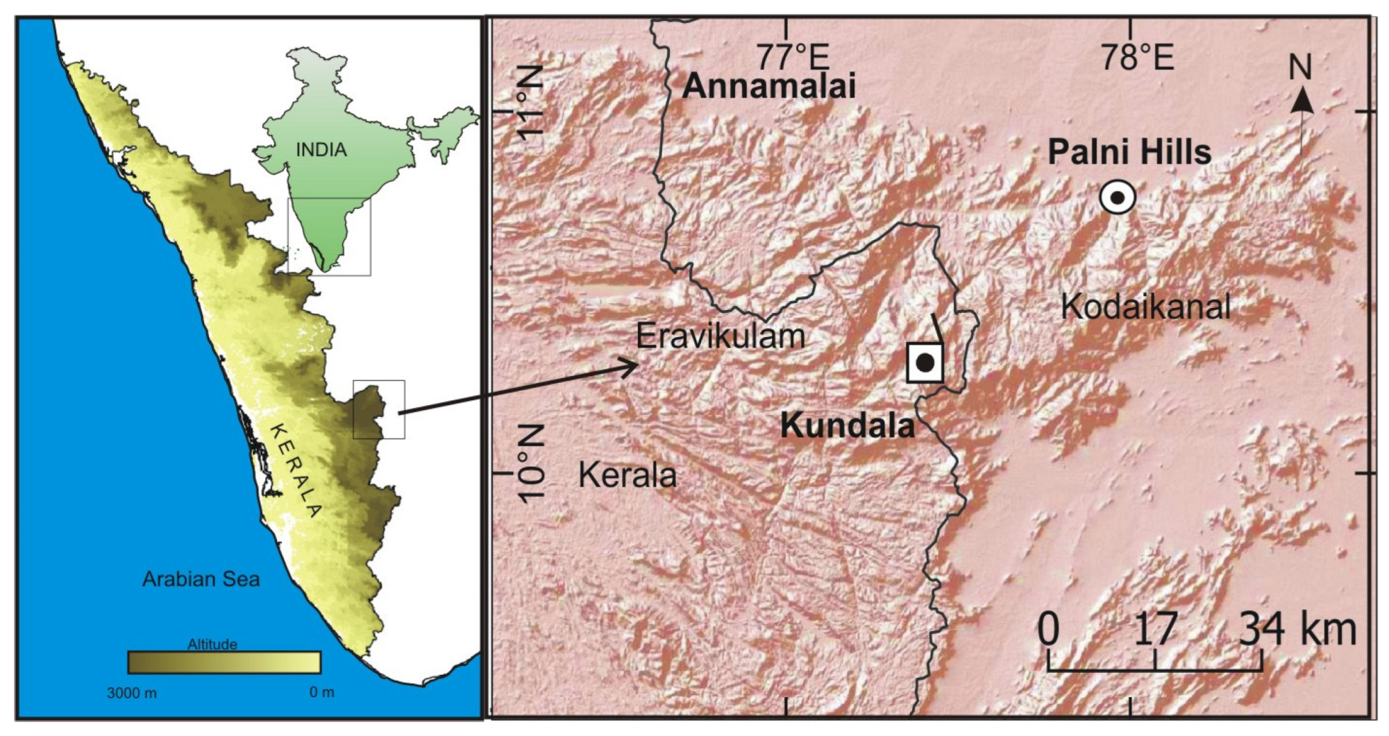
2. Study Area
3. Materials and Methods
3.1. Chronology of Sediment Core (Kundala Lake)
3.2. Palynological Study
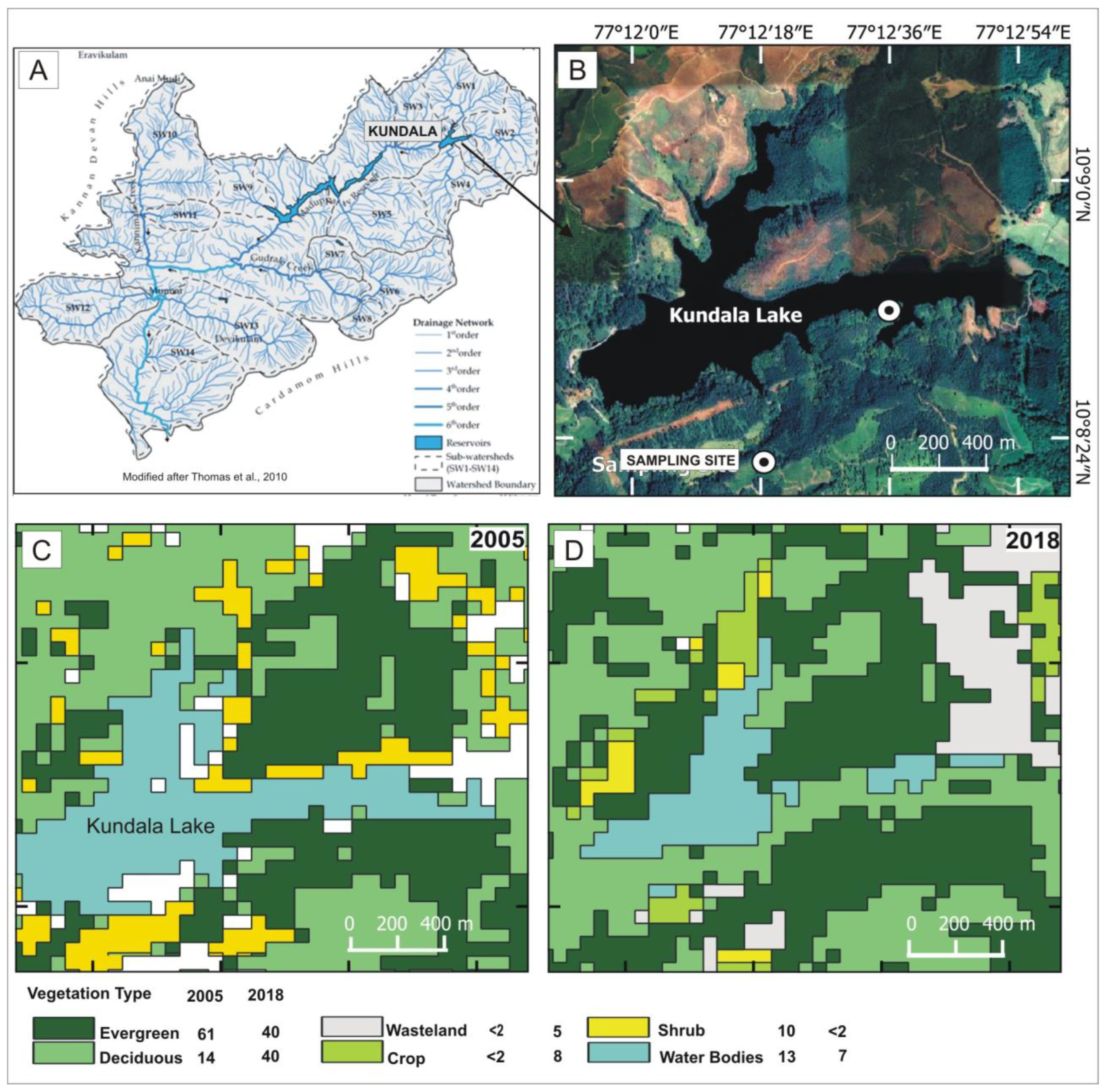
3.3. Modern Vegetation Cover
3.4. Estimation of Mean Annual Temperature (MAT) and Mean Annual Precipitation (MAP)
4. Results
4.1. Chronology of Kundala Lake Sedimentary Profile
4.2. Palynology (Kundala Lake)
4.2.1. Phase I (4.3–3.4 ka)
4.2.2. Phase II (3.4–2.3 ka)
4.2.3. Phase III (2.3–0.9 ka)
4.2.4. Phase IV (0.9–0.12 ka)
4.2.5. Phase V (Since ~0.12 ka)
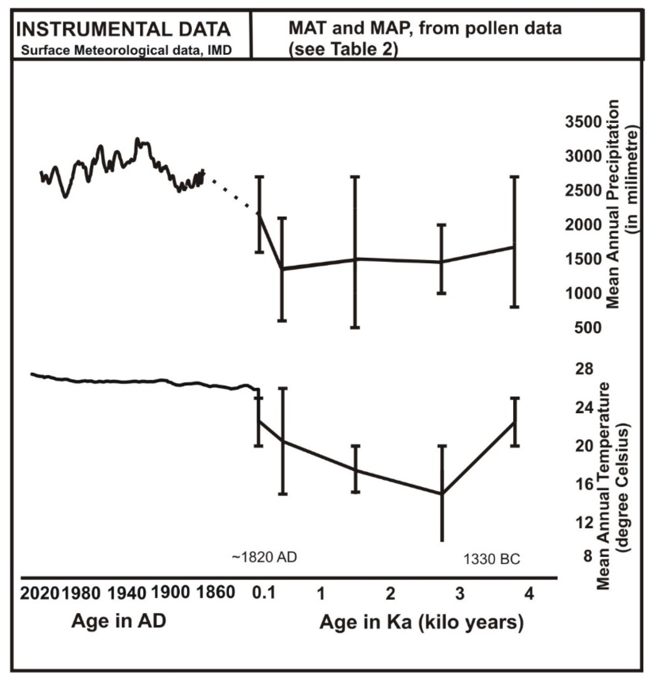
4.3. MAT and MAP
4.4. DEM Analysis of Kundala Lake Site
4.5. Temperature and Precipitation—Instrumental Record Post 1820AD
5. Discussion
5.1. Climate–Vegetation Relationship Since Middle Holocene, Southern Western Ghats
5.2. Climate–Vegetation Relationship Since ~1820 AD, Kerala
6. Conclusions
Author Contributions
Funding
Data Availability Statement
Acknowledgments
Conflicts of Interest
References
- Lisiecki, L.E.; Raymo, M.E. A Pliocene–Pleistocene stack of 57 globally distributed benthic δ18O records. Paleoceanography 2005, 20, PA1003. [Google Scholar] [CrossRef]
- Martinson, D.G.; Pisias, N.G.; Hays, J.D.; Imbrie, J.D.; Moore, T.C.; Shackleton, N.J. Age Dating and the orbital theory of the ice ages: Development of a high-resolution 0 to 300,000-year chronostratigraphy. Quat. Res. 1987, 27, 1–29. [Google Scholar] [CrossRef]
- Naidu, P.D.; Malmgren, B.A. 2,200 years periodicity in the Asian monsoon system. Geophys. Res. Lett. 1995, 22, 2361–2364. [Google Scholar] [CrossRef]
- Nigam, R.; Khare, N.; Nair, R.R. Foraminiferal evidences for 77–year cycles of droughts in India and its possible modulation by the Gleissberg solar cycle. J. Coast. Res. 1995, 11, 1099–1107. [Google Scholar]
- Weiskopf, S.R.; Rubenstein, M.A.; Lisa, G.; Crozier, L.G.; Gaichas, S.; Griffis, R.; Halofsky, J.E.; Hyde, K.J.; Morelli, T.L.; Morisette, J.T.; et al. Climate change effects on biodiversity, ecosystems, ecosystem services, and natural resource management in the United States. Sci. Total Environ. 2020, 733, 137782. [Google Scholar]
- Capua, G.D.; Kretschmer, M.; Reik, V.; Donner, R.V.; van den Hurk, B.; Ramesh Vellore, R.; Raghavan Krishnan, R.; Coumou, D. Tropical and mid–latitude teleconnections interacting with the Indian summer monsoon rainfall: A theory-guided causal effect network approach. Earth Syst. Dynam. 2020, 11, 17–34. [Google Scholar] [CrossRef]
- Choudhury, A.K.; Krishnan, R. Dynamical Response of the South Asian Monsoon Trough to Latent Heating from Stratiform and Convective Precipitation. J. Atmos. Sci. 2011, 68, 1347–1363. [Google Scholar]
- Kiladis, G.; Diaz, H.F. Global Climatic Anomalies Associated with Extremes in the Southern Oscillation. J. Clim. 1989, 2, 1069–1090. [Google Scholar]
- Ali, S.N.; Dubey, J.; Ghosh, R.; Quamar, M.F.; Sharma, A.; Morthekai, P.; Dimri, A.P. High frequency abrupt shifts in the Indian summer monsoon since Younger Dryas in the Himalaya. Sci. Rep. 2018, 8, 9287. [Google Scholar] [CrossRef]
- Cullen, H.M.; Hemming, S.; Hemming, G.; Brown, F.; Guilderson, T.; Sirocko, F. Climate change and the collapse of the Akkadian empire: Evidence from the deep sea. Geology 2000, 28, 379–382. [Google Scholar]
- Dixit, Y.; Hodell, D.A.; Giesche, A.; Tandon, S.K.; Gázquez, F.; Saini, H.S.; Skinner, L.C.; Mujtaba, S.A.; Pawar, V.; Singh, R.N. Intensified summer monsoon and the urbanization of Indus Civilization in northwest India. Sci. Rep. 2018, 8, 4225. [Google Scholar] [CrossRef]
- Giosan, L.; Pete, D.; Mark, C.; Macklin, G.; Fuller, D.Q.; Constantinescu, S.; Julie, A.; Thomas, D.; Stevens, G.; Duller, A.T.; et al. Fluvial landscapes of the Harappan civilization. Proc. Natl. Acad. Sci. USA 2012, 109, E1688–E1694. [Google Scholar] [CrossRef]
- Kathayat, G.; Cheng, H.; Sinha, A.; Berkelhammer, M.; Zhang, H.; Duan, P.; Li, H.; Li, X.; Ning, Y.; Edwards, R.L. Evaluating the timing and structure of the 4.2 ka event in the Indian summer monsoon domain from an annually resolved speleothem record from Northeast India. Clim. Past 2018, 14, 1869–1879. [Google Scholar] [CrossRef]
- Nakamura, T.; Yamazaki, K.; Iwamoto, K.; Honda, M.; Miyoshi, Y.; Ogawa, Y.; Tomikawa, Y.; Ukita, J. The stratospheric pathway for Arctic impacts on midlatitude climate. Geophys. Res. Lett. 2016, 43, 3494–3501. [Google Scholar] [CrossRef]
- Fleitmann, D.; Burns, S.; Augusto, M.; Mudelsee, M.; Kramers, J.; Villa, I.; Ulrich, N.; Al-Subbary, A.A.; Buettner, A.; Hippler, D.; et al. Holocene ITCZ and Indian Monsoon Dynamics Recorded in Stalagmites from Oman and Yemen (Socotra). Quat. Sci. Rev. 2007, 26, 170–188. [Google Scholar] [CrossRef]
- Gadgil, S. The Indian Monsoon Variability. Annu. Rev. Earth Planet. Sci. 2003, 31, 429–467. [Google Scholar] [CrossRef]
- Allen, C.; Macalady, A.; Bachelet, D.; McDowell, N.; Vennetier, M.; Kitzberger, T.; Rigling, A.; Breshears, D.; Hogg EHGonzalez, P.; Fensham, R.; et al. A global overview of drought and heat–induced tree mortality reveals emerging climate change risks for forests. For. Ecol. Manag. 2010, 259, 660–684. [Google Scholar] [CrossRef]
- Murphy, B.F.; Timbal, B. A review of recent climate variability and climate change in southeastern Australia. Int. J. Climatol. 2007, 28, 859–879. [Google Scholar] [CrossRef]
- Nicholls, N.; Lavery, B. Australian rainfall trends during the twentieth century. Int. J. Climatol. 2006, 12, 153–163. [Google Scholar] [CrossRef]
- Nicholson, S.E.; Grist, J.P. A conceptual model for understanding rainfall variability in the West African Sahel on interannual and interdecadal timescales. Int. J. Climatol. 2001, 21, 1733–1757. [Google Scholar] [CrossRef]
- Rodrigo, S.; Esteban–Parra, M.J.; Pozo–Va’zquez, D.; Castro–Dı’ez, Y. Rainfall variability in southern Spain on decadal to centennial time scales. Int. J. Climatol. 2000, 20, 721–732. [Google Scholar]
- Rotstayn, L.D.; Lohmann, U. Tropical rainfall trends and the indirect aerosol effect. J. Clim. 2002, 15, 2103–2116. [Google Scholar] [CrossRef]
- Alvi, S.M.A.; Koteswaram, P. Time series analysis of annual rainfall over India. Mausam 1985, 36, 479–490. [Google Scholar] [CrossRef]
- Parthasarathy, B.; Mooley, D.A. Some features of a long homogeneous series of Indian summer monsoon rainfall. Mon. Weather Rev. 1978, 106, 771–781. [Google Scholar] [CrossRef]
- Thapliyal, V.; Kulshrestha, S.M. Climate changes and trends over India. Mausam 1991, 42, 333–338. [Google Scholar] [CrossRef]
- Akhoury, G.; Avishek, K. Climatic changes over the Arabian Peninsula and their correlation with Indian rainfall. J. Earth Syst. Sci. 2019, 128, 147. [Google Scholar] [CrossRef]
- Kothawale, D.R.; Rajeevan, M. Monthly, Seasonal and Annual Rainfall Time Series for All–India, Homogeneous Regions and Meteorological Subdivisions; A Contribution from IITM, Research Report No. RR-138, ESSO/IITM/STCVP/SR/02(2017)/189; Indian Institute of Tropical Meteorology: Pune, India, 2017; pp. 1871–2016. ISSN 0252–1075. [Google Scholar]
- IPCC. Climate Change 2007. Synthesis Report. Contribution of Working Groups I, II & III to the Fourth Assessment Report of the Intergovernmental Panel on Climate Change; IPCC: Geneva, Switzerland, 2007. [Google Scholar] [CrossRef]
- Rao, V.B.; Ferreira, C.C.; Franchito, S.H.; Ramakrishna, S.S.V.S. In a changing climate weakening tropical easterly jet induces more violent tropical storms over the north Indian Ocean. Geophys. Res. Lett. 2008, 35, L15710. [Google Scholar] [CrossRef]
- Sathiyamoorthy, V. Large scale reduction in the size of the Tropical Easterly Jet. Geophys. Res. Lett. 2005, 32, L14802. [Google Scholar] [CrossRef]
- Rajendran, K.; Kitoh, A.; Srinivasan, J.; Mizuta, R.; Raghavan, K. Monsoon circulation interaction with Western Ghats orography under changing climate: Projection by a 20–km mesh AGCM. Theor. Appl. Clim. 2012, 110, 555–571. [Google Scholar] [CrossRef]
- Meir, P.; Wood, T.E.; Galbraith, D.R.; Brando, P.M.; Da Costa, A.C.L.; Rowland, L.; Ferreira, L.V. Threshold responses to soil moisture deficit by trees and soil in tropical rain forests: Insights from field experiments. BioScience 2015, 65, 882–892. [Google Scholar]
- Barboni, D.; Bonnefille, R.; Prasad, S.; Ramesh, B. Variation in modern pollen from tropical evergreen forests and the monsoon seasonality gradient in SW India. J. Veg. Sci. 2003, 14, 551–562. [Google Scholar] [CrossRef]
- Bera, S.K.; Farooqui, A. Mid–Holocene vegetation and climate of South Indian Montane. J. Palaeontol. Soc. India 2000, 45, 49–56. [Google Scholar] [CrossRef]
- Blasco, F.; Thanikaimoni, G. Late Quaternary vegetational history of southern region. In Aspects and Appraisal of Indian Palaeobotany; Surange, K.R., Lakhanpal, R.N., Bharadwaj, D.C., Eds.; B.S.I.P.: Lucknow, India, 1974; pp. 632–643. [Google Scholar]
- Farooqui, A.; Ray, J.G.; Farooqui, S.A.; Tiwari, R.K.; Khan, Z.A. Tropical rainforest vegetation, climate and sea level during the Pleistocene in Kerala, India. Quat. Int. 2010, 213, 2–11. [Google Scholar]
- Thomas, J.; Joseph, S.; Thrivikramaji, K.P. Morphometric aspects of a small tropical mountain river system, the southern Western Ghats, India. Int. J. Digit. Earth 2010, 3, 135–156. [Google Scholar]
- Vishnu–Mittre, V.M.; Gupta, H.P. A living fossil plant community in South Indian Hills. Curr. Sci. 1968, 37, 671–672. [Google Scholar]
- Prasad, V.; Farooqui, A.; Tripathi, S.K.M.; Garg, R.; Thakur, B. Evidence of Late Palaeocene–Early Eocene equatorial rain forest refugia in southern western Ghats, India. J. Biosci. 2009, 34, 777–797. [Google Scholar]
- Ramanujam, C.G.K. Palynology of the Neogene Warkalli Beds of Kerala State in South India. J. Palaeontol. Soc. India 1987, 32, 26–46. [Google Scholar]
- Ganesh, T.Z.; Ganesam, M.; Devy, S.; Davida, P.; Bawa, K.S. Assessment of plant biodiversity at a mid–elevation evergreen forest of Kalakad–Mundanthurai Tiger reserve,Western ghats, India. Curr. Sci. 1996, 71, 379–391. [Google Scholar]
- Ghate, U.; Joshi, N.V.; Gadgil, M. On the patterns of tree diversity in the western ghats of India. Curr. Sci. 1998, 75, 594–603. [Google Scholar]
- Ramesh, B.R.; Pascal, J.P. Atlas of Endemics of the Western Ghats (India); Institute Francais de Pondichery: Pondicherry, India, 1997. [Google Scholar]
- Reimer, P.J.; Austin, W.E.N.; Bard, E.; Bayliss, A.; Blackwell, P.G.; Ramsey, C.B.; Butzin, M.; Cheng, H.; Edwards, R.L.; Friedrich, M.; et al. The INTCAL20 Northern Hemisphere Radiocarbon age calibration curve (0–55 Cal kBP). Radiocarbon 2020, 62, 1–33. [Google Scholar]
- Stuiver, M.; Reimer, P.J.; Bard, E.; Beck, J.W.; Burr, G.S.; Hughen, K.A.; Kromer, B.; McCormac, G.; Van Der Plicht, J.; Spurk, M. INTCAL98 radiocarbon age calibration, 24,000–0 cal BP. Radiocarbon 1998, 40, 1041–1083. [Google Scholar]
- Blaauw, M. Methods and code for “classical” age–modeling of radiocarbon sequences. Quat. Geochronol. 2010, 5, 512–518. [Google Scholar] [CrossRef]
- Erdtman, G. An Introduction to Pollen Analysis; Chronica Botanica Company: Waltham, MA, USA, 1943; pp. 1–239. [Google Scholar]
- Grimm, E. Tilia Program Ver. 2.0 B4; Springfield: Springfield, IL, USA, 1991. [Google Scholar]
- Mosbrugger, V.; Utescher, T. The coexistence approach—A method for quantitative reconstructions of Tertiary terrestrial palaeoclimate data using plant fossils. Palaeogeogr. Palaeoclimatol. Palaeoecol. 1997, 134, 61–86. [Google Scholar]
- Utescher, T.; Bruch, A.A.; Erdei, B.; François, L.; Ivanov, D.; Jacques, F.M.B.; Kern, A.K.; Mosbrugger, V.; Spicer, R.A. The Coexistence Approach—Theoretical background and practical considerations of using plant fossils for climate quantification. Palaeogeogr. Palaeoclimatol. Palaeoecol. 2014, 410, 58–73. [Google Scholar]
- Champion, H.G.; Seth, S.K. A Revised Survey of Forest Types of India; Government of India: Delhi, India, 1968.
- Walter, P. Diurnal and nocturnal flight activity of Scarabaeinecoprophages in tropical Africa. Rev. Int. De Géologie De Géographie Et D’écologietropicales 1985, 9, 67–87. [Google Scholar]
- Farooqui, A.; Khan, S.; Agnihotri, R.; Phartiyal, B.; Shukla, S. Monitoring hydrecology and climatic variability since ~4.6 ka from palynological, sedimentological and environmental perspectives in an Ox–bow lake Central Ganga Plain, India. Holocene 2023, 33, 1272–1288. [Google Scholar] [CrossRef]
- Chaturvedi, R.K.; Gopalakrishnan, R.; Jayaraman, M.; Bala, G.; Joshi, N.V.; Sukumar, R.; Ravindranath, N.H. Impact of climate change on Indian forests: A dynamic vegetation modeling approach. Mitig. Adapt. Strateg. Glob. Change 2011, 16, 119–142. [Google Scholar]
- Foley, J.A.; DeFries, R.; Asner, G.P.; Barford, C.; Bonan, G.; Carpenter, S.R.; Chapin, F.S.; Coe, M.T.; Daily, G.C.; Gibbs, H.K.; et al. Global consequences of land use. Science 2005, 309, 570–574. [Google Scholar]
- Cramer, W.; Bondeau, A.; Woodward, F.I.; Prentice, I.C.; Betts, R.A.; Brovkin, V.; Cox, P.M.; Fisher, V.; Foley, J.A.; Friend, A.D.; et al. Global response of terrestrial ecosystem structure and function to CO2 and climate change: Results from six dynamic global vegetation models. Glob. Change Biol. 2001, 7, 357–373. [Google Scholar]
- McGuire, A.D.; Sitch, S.; Clein, J.S.; Dargaville, R.; Esser, G.; Foley, J.; Heimann, M.; Joos, F.; Kaplan, J.; Kicklighter, D.W.; et al. Carbon balance of the terrestrial biosphere in the twentieth century: Analyses of CO2, climate and land use effects with four process–based ecosystem models. Glob. Biogeochem. Cycles 2001, 15, 183–206. [Google Scholar]
- India Meterological Office. Climatological Tables of Observatories in India, 1931–1960; India Meterological Office: New Delhi, India, 1967; Volume xxii, p. 470. [Google Scholar]
- Mini, V.K.; Pushpa, V.L.; Manoj, K.B. Inter–annual and Long term Variability of Rainfall in Kerala India Meteorological Department Thiruvananthapuram. Vayu Mandal 2016, 42, 32–42. [Google Scholar]
- Andreu, L.; Gutierrez, E.; Macias, M.; Ribas, M.; Bosch, O.; Camarero, J.J. Climate increases regional tree–growth variability in Iberian pine forests. Glob. Change Biol. 2007, 13, 804–815. [Google Scholar] [CrossRef]
- Polgar, C.A.; Primack, R.B. Leaf–out phenology of temperate woody plants: From trees to ecosystems. New Phytol. 2011, 191, 926–941. [Google Scholar] [CrossRef]
- Achyuthan, H.; Farooqui, A.; Gopal, V.; Phartiyal, B.; Lone, A.M. Late Quaternary to Holocene Southwest Monsoon Reconstruction: A Review Based on Lake and Wetland Systems. Proc. Indian Natl. Sci. Acad. 2016, 82, 847–868. [Google Scholar]
- Dixit, Y.; Hodell, D.A.; Petrie, C.A. Abrupt weakening of the summer monsoon in northwest India 4100 yr ago. Geology 2014, 42, 339–342. [Google Scholar] [CrossRef]
- Dixit, Y.; Tandon, S. Hydroclimatic variability on the Indian–subcontinent in the past millennium: Review and assessment. Earth–Sci. Rev. 2016, 161, 1–5. [Google Scholar] [CrossRef]
- Farooqui, A.; Ranjana; Nautiyal, C.M. Deltaic land subsidence and sea level fluctuations along the east coast of India since 8 ka: A palynological study. Holocene 2016, 26, 1426–1437. [Google Scholar]
- Misra, P.; Farooqui, A.; Sinha, R.; Sonal, K.; Tandon, S. Millennial–scale vegetation and climatic changes from an Early to Mid–Holocene lacustrine archive in Central Ganga Plains using multiple biotic proxies. Quat. Sci. Rev. 2020, 243, 106474. [Google Scholar] [CrossRef]
- Phartiyal, B.; Farooqui, A.; Bose, T. Climate Change Variability Through Lacustrine Records Published During 2016–2019: Implications, New Approaches, and Future Direction. Proc. Indian Natl. Sci. Acad. 2020, 86, 389–403. [Google Scholar] [CrossRef]
- Pokharia, A.K.; Agnihotri, R.; Sharma, S.; Bajpai, S.; Nath, J.; Kumaran, R.N.; Negi, B.C. Altered cropping pattern and cultural continuation with declined prosperity following abrupt and extreme arid event at ~4200 yrs BP: Evidence from an Indus archaeological site Khirsara, Gujarat, western India. PLoS ONE 2017, 12, e0185684. [Google Scholar] [CrossRef]
- Sengupta, T.; Deshpande, M.A.; Bhushan, R.; Ram, F.; Bera, M.K.; RajAnkur Dabhi, H.; Bisht, R.S.; Rawat, Y.S.; Bhattacharya, S.K.; Juyal, N.; et al. Did the Harappan settlement of Dholavira (India) collapse during the onset of Meghalayan stage drought? J. Quat. Sci. 2019, 35, 1–14. [Google Scholar] [CrossRef]
- Walker, M.C.J.; Berkelhammer, M.; Bjork, S.; Cwynar, L.C.; Fisher, D.A.; Weiss, H. Formal subdivision of the Holocene Series/Epoch: A Discussion Paper by a Working Group of INTIMATE (Integration of ice–core, marine and terrestrial records) and the Subcommission on Quaternary Stratigraphy (International Commission on Stratigraphy). J. Quat. Sci. 2012, 27, 649–659. [Google Scholar] [CrossRef]
- Prasad, S.; Kusumgar, S.; Gupta, S.K. A mid to late Holocene record of paleoclimatic changes from Nal Sarovar, a paleodesert margin lake in Western India. J. Quat. Sci. 1997, 12, 153–159. [Google Scholar] [CrossRef]
- Kajale, M.D.; Deotare, B.C. Late Quaternary environmental studies on salt lakes in western Rajasthan, India: A summarised view. J. Quat. Sci. 1997, 12, 405–412. [Google Scholar] [CrossRef]
- Staubwasser, M.; Sirocko, F.; Grootes, P.; Segl, M. Climate change at the 4.2 ka BP termination of the Indus valley civilization and Holocene south Asian monsoon variability. Geophys. Res. Lett. 2003, 30, 1425. [Google Scholar] [CrossRef]
- Kaufman, D.; McKay, N.; Zhilich, S. A global database of Holocene paleotemperature records. Sci. Data 2020, 7, 115. [Google Scholar] [CrossRef]
- Trivedi, A.; Tang, Y.-N.; Fen, Q.; Farooqui, A.; Alexandra, W.; Wang, Y.-F.; Blackmore, S.; Li, C.-S.; Yao, Y.-F. Holocene vegetation dynamics and climatic fluctuations from Shuanghaizi Lake in the Hengduan Mountains, southwestern China. Palaeogeogr. Palaeoclimatol. Palaeoecol. 2020, 560, 110035. [Google Scholar] [CrossRef]
- Bartlein, P.J.; Harrison, S.P.; Brewer, S.; Connor, S.; Davis, B.A.S.; Gajewski, K.; Guiot, J.; Harrison-Prentice, T.I.; Henderson, A.; Peyron, O.; et al. Pollen-based continental climate reconstructions at 6 and 21 ka: A global synthesis. Clim. Dyn. 2011, 37, 775–802. [Google Scholar] [CrossRef]
- Harrison, S.P.; Bartlein, P.J.; Brewer, S.; Prentice, I.C.; Boyd, M.; Hessler, I.; Holmgren, K.; Izumi, K.; Willis, K. Climate model benchmarking with glacial and mid-Holocene climates. Clim. Dyn. 2014, 43, 671–688. [Google Scholar] [CrossRef]
- Mauri, A.; Davis, B.A.S.; Collins, P.M.; Kaplan, J.O. The climate of Europe during the Holocene: A gridded pollen–based reconstruction and its multiproxy evaluation. Quat. Sci. Rev. 2015, 112, 109–127. [Google Scholar] [CrossRef]
- Viau, A.E.; Gajewski, K.; Sawada, M.C.; Fines, P. Millennial–scale temperature variations in North America during the Holocene. J. Geophys. Res. Atmos. 2006, 111, D09102. [Google Scholar] [CrossRef]
- Krishnakumar, K.N.; Prasada Rao, G.S.L.H.V.; Gopakumar, C.S. Rainfall trends in twentieth century over Kerala, India. In Atmospheric Environment; Elsevier Ltd.: Amsterdam, The Netherlands, 2009; Volume 43, pp. 1940–1944. ISSN 1352-2310. [Google Scholar] [CrossRef]
- Singh, O.P. Recent trends in tropical cyclone activity in the North Indian Ocean. In Indian Ocean Tropical Cyclones and Climate Change; Springer: Dordrecht, The Netherlands, 2010; pp. 51–54. [Google Scholar]
- Jeong, S.; Ho, C.; Gim, H.; Brown, M.E. Phenology shifts at start vs. end of growing season in temperate vegetation over the Northern Hemisphere for the period 1982–2008. Glob. Change Biol. 2011, 17, 2385–2399. [Google Scholar] [CrossRef]
- Wang, X.; Piao, S.; Ciais, P.; Li, J.; Friedlingstein, P.; Koven, C.; Chen, A. Spring temperature change and its implication in the change of vegetation growth in North America from 1982 to 2006. Proc. Natl. Acad. Sci. USA 2011, 108, 1240–1245. [Google Scholar]
- Hofhans, F.; Chacón–Madrigal, E.; Fuchslueger, L.; Jenking, D.; Morera-Beita, A.; Plutzar, C.; Silla, F.; Andersen, K.M.; Buchs, D.M.; Dullinger, S.; et al. Climatic and edaphic controls over tropical forest diversity and vegetation carbon storage. Sci. Rep. 2020, 10, 5066. [Google Scholar] [CrossRef]
- Choat, B.; Jansen, S.; Brodribb, T.J.; Cochard, H.; Delzon, S.; Bhaskar, R.; Bucci, S.J.; Feild, T.S.; Gleason, S.M.; Hacke, U.G.; et al. Global convergence in the vulnerability of forests to drought. Nature 2012, 491, 752–755. [Google Scholar] [CrossRef] [PubMed]
- Farooqui, A.; Agnihotri, R.; Khan, S.; Gahlaud, S.K.S.; Sharief, M.U. Temporal variability in carbon and nitrogen stable isotopes of Strobilanthes kunthianus leaf: Its photosynthetic efficacy and water–use efficiency in a warming climate. J. Earth Syst. Sci. 2021, 130, 241. [Google Scholar] [CrossRef]
- Wu, Z.; Dijkstra, P.; Koch, G.W.; Peñuelas, J.; Hungate, B.A. Responses of terrestrial ecosystems to temperature and precipitation change: A meta–analysis of experimental manipulation. Glob. Change Biol. 2011, 17, 927–942. [Google Scholar] [CrossRef]
- Graven, H.; Allison, C.E.; Etheridge, D.M.; Hammer, S.; Keeling, R.F.; Levin, I.; Harro, A.J.M.; Rubino, M.; Tans, P.P.; Trudinger, C.M.; et al. Compiled records of carbon isotopes in atmospheric CO2 for historical simulations in CMIP6. Geosci. Model Dev. 2017, 10, 4405–4417. [Google Scholar] [CrossRef]


| Depth in cm | Birbal Sahni (BS) Institute Laboratory | Radiocarbon Age (Years BP: Before Present) * | Calibrated Calendar Years |
|---|---|---|---|
| 0–10 (Phase V) | 0–124 | ||
| 20–25 | BS–4027 | 310 ± 60 * | 1557 AD |
| 10–35 (Phase IV) | 124–868 | ||
| 35–60 (Phase III) | 868–2263 | ||
| 70–75 | BS–3780 | 3100 ± 190 * | 1110 BC |
| 60–85 (Phase II) | 2263–3367 | ||
| 85–120 (Phase I) | 3367–4300 | ||
| 115–120 | BS–3779 | 4300 ± 310 * | 2350 BC |
| Mean Annual Temperature (°C) | Mean Annual Precipitation (mm) | Evergreen, Semi-Evergreen/Moist Deciduous Taxa (Shola Forest and Plant Associates) |
|---|---|---|
| 15–30 | 2000–3000 | Aglaia |
| 20–35 | Up to 3000 | Anacardium |
| 15–25 | Up to 2500 | Bignoniaceae |
| 15–25 | 1500–2500 | Chrysophyllum |
| 15–30 | 1000–2500 | Acacia |
| 15–25 | 1200–2500 | Agrostistachys |
| 20–35 | 1000–3000 | Anacardiacea |
| 15–25 | 1500–3000 | Annonaceae |
| 15–25 | 1200–2500 | Arecaceae |
| 15–25 | 1000–2000 | Baccaurea |
| 10–32 | 1100–3000 | Bombax ceiba |
| 15–25 | 1000–2500 | Basella keralensis |
| 15–25 | ~2500 | Caesalpiniaceae |
| 15–25 | ~2200 | Canarium |
| 10–20 | ~2200 | Casuarina |
| 10–20 | 1500–2500 | Celastraceae |
| 10–25 | 1000–2000 | Dillenia |
| 22–35 | 1500–2500 | Dipterocarpaceae |
| 22–33 | 1500–2500 | Dodonaea |
| 5–20 | 1000–2000 | Duabanga |
| 10–20 | 1500–3000 | Dysoxylum |
| 15–30 | 1500–3000 | Elaeocarpus |
| 10–20 | 1500–3000 | Eucalyptus |
| 25–31 | 2500–4500 | Euonymous |
| 5–28 | 1500–3000 | Eurya |
| 10–20 | Up to 3000 | Garcinia |
| 25–35 | Up to 3000 | Garuga |
| 10–20 | 1500–3000 | Gentianaceae |
| 10–25 | ~3000 | Gluta |
| 10–25 | 1500–2500 | Hopea |
| 5–25 | 1500–3000 | Humboldtia, |
| 10–25 | 500–4000 | Ilex |
| 5–20 | Up to 3000 | Knema |
| 10–25 | 500–1600 | Ligustrum |
| 5–20 | 1000–2000 | Limonia |
| 10–20 | 1000–2000 | Lophopetalum |
| 10–20 | 500–2500 | Luvunga |
| 16–28 | 500–2000 | Mallotus |
| 10–40 | 500–2500 | Mangifera indica |
| 6–35 | 500–3500 | Meliaceae |
| 5–25 | 500–3000 | Mesua |
| 13–36 | 500–4000 | Moraceae |
| 10–25 | 1500–2500 | Murraya |
| 10–25 | 500–3000 | Myrtaceae |
| 10–25 | 500–2600 | Nothapodytes |
| 10–25 | 500–2500 | Nothopegia |
| 5–25 | 500–2500 | Oleaceae |
| 6–31 | 2500–4500 | Osbeckia |
| 10–25 | 1000–2500 | Ongoeckia gore |
| 10–25 | ~3000 | Palaquim |
| 5–20 | 1000–2500 | Pinus |
| 10–25 | 1000–2500 | Psychotria |
| 10–25 | ~3500 | Reinwardtiodendron |
| 12–25 | 1500–2500 | Rhododendron |
| 20–35 | 1000–2000 | Sapotacea |
| 25–40 | 1000–3000 | Schleichera |
| 10–25 | Up to 3000 | Scolopia |
| 10–25 | Up to 2500 | Semecarpus |
| 5–20 | 1500–2500 | Shorea |
| 5–20 | 1000–3000 | Sterculiaceae |
| 10–25 | 1500–2500 | Striga augustifolia |
| 20–30 | 2000–3000 | Symplocos |
| 13–28 | 1500–3000 | Syzygium |
| 10–25 | 1000–2000 | Terminalia |
| 10–25 | 1000–2500 | Tiliaceae |
| 5–20 | 1000–2500 | Trema |
| 5–20 | 1000–2500 | Turpinia |
| Dry deciduous taxa | ||
| 18–30 | 500–1500 | Fabaceae |
| 15–28 | 1000–2000 | Lagerstoemia |
| 5–15 | 1000–2000 | Madhuca |
| 5–15 | Up to 1500 | Ricinus |
| Herbaceous and woody shrubs | ||
| Rutaceae, | ||
| 10–20 | 1500–2500 | Ericaceae |
| 10–25 | 2000–3000 | Ixora |
| 10–20 | 1000–2000 | Apiaceae |
| 17–35 | 1000–2000 | Euphorbia |
| 10–25 | 1000–2000 | Hibiscus |
| 12–27 | 500–2000 | Hypericum |
| 10–20 | 500–2000 | Lythraceae |
| 10–20 | 500–1500 | Neonotis |
| 10–20 | 1000–2000 | Senecio |
| 13–28 | 500–2000 | Launea |
| 5–25 | 500–1500 | Myristica |
| 5–15 | 1000–2000 | Blumea |
| 12–20 | 1000–2000 | Campanula |
| 15–35 | Up to 2000 | Centratherum |
| 5–15 | 500–1500 | Chenopodiaceae |
| 5–25 | 500–2000 | Cnicus |
| 15–40 | 800–2000 | Combretacea |
| 18–30 | 500–1500 | Eriocaulon |
| 5–15 | 500–1500 | Erythrina |
| 5–15 | 500–2000 | Pedicularis |
| 9–22 | 1000–2000 | Pimpinella |
| 10–20 | 500–1500 | Ranunculaceae |
| 5–20 | 500–1500 | Rosaceae |
| 15–28 | 800–2500 | Rubiaceae |
| 22–32 | 1000–3000 | Strobilanthes |
| 15–25 | 850–2200 | Vernonia |
| 12–40 | 800–1500 | Boerhavia |
| 5–20 | 850–2200 | Heracleum |
| 10–20 | 500–1500 | Tabernaemontana |
| 5–20 | 1000–2000 | Impatiens |
| 15–30 | 1000–2000 | Jasminuim |
| 5–15 | 1500–2500 | Lamiaceae |
| 5–15 | 1500–3500 | Liliaceae, |
| 10–20 | 1500–3500 | Clerodendrum |
| 5–20 | 1500–2500 | Cucurbitaceae |
| 20–30 | 1500–3500 | Derris |
| 5–20 | 500–2000 | Caryophyllaceae, |
| 10–15 | 1000–2000 | Chlorophytum |
| 17–35 | 500–2500 | Justicia |
| 10–20 | 500–2500 | Solanaceae |
| 15–30 | 1500–3000 | Tinospora |
| 20–30 | 1500–3000 | Urticaceae, |
| 10–25 | 500–2500 | Xanthium |
| 5–15 | 500–3500 | Cyperaceae |
| 5–25 | 1000–4000 | Poaceae |
| 500–2500 | Aquatic | |
| 8–12 | Polygala | |
| 5–18 | Myriophyllum | |
| 5–25 | Nuphar | |
| 15–35 | Polygonum | |
| 10–25 | Potamogeton | |
| 10–30 | Typha | |
| 10–26 | Lemna |
Disclaimer/Publisher’s Note: The statements, opinions and data contained in all publications are solely those of the individual author(s) and contributor(s) and not of MDPI and/or the editor(s). MDPI and/or the editor(s) disclaim responsibility for any injury to people or property resulting from any ideas, methods, instructions or products referred to in the content. |
© 2025 by the authors. Licensee MDPI, Basel, Switzerland. This article is an open access article distributed under the terms and conditions of the Creative Commons Attribution (CC BY) license (https://creativecommons.org/licenses/by/4.0/).
Share and Cite
Farooqui, A.; Khan, S. Evaluation of Temperature and Precipitation Since 4.3 ka Using Palynological Data from Kundala Lake Sediments, Kerala, India. Quaternary 2025, 8, 17. https://doi.org/10.3390/quat8020017
Farooqui A, Khan S. Evaluation of Temperature and Precipitation Since 4.3 ka Using Palynological Data from Kundala Lake Sediments, Kerala, India. Quaternary. 2025; 8(2):17. https://doi.org/10.3390/quat8020017
Chicago/Turabian StyleFarooqui, Anjum, and Salman Khan. 2025. "Evaluation of Temperature and Precipitation Since 4.3 ka Using Palynological Data from Kundala Lake Sediments, Kerala, India" Quaternary 8, no. 2: 17. https://doi.org/10.3390/quat8020017
APA StyleFarooqui, A., & Khan, S. (2025). Evaluation of Temperature and Precipitation Since 4.3 ka Using Palynological Data from Kundala Lake Sediments, Kerala, India. Quaternary, 8(2), 17. https://doi.org/10.3390/quat8020017