Why Is the Linearized Form of Pseudo-Second Order Adsorption Kinetic Model So Successful in Fitting Batch Adsorption Experimental Data?

Abstract

There is a vast amount of literature devoted to experimental studies on adsorption from liquids examining the adsorption potential of various adsorbents with respect to various solutes. Most of these studies contain not only equilibrium but also kinetic experimental data. The standard procedure followed in the literature is to fit the kinetic experimental adsorption data to some models. Typically empirical models are employed for this purpose and among them, the pseudo-first and pseudo-second order kinetic models are the most extensively used. In particular, the linear form of their integrated equations is extensively employed. In most cases, it is found that the pseudo-second order model is not only better than other models but also leads to high fitting quality. This is rather strange since there is no physical justification for such a model, as it is well accepted that adsorption kinetics is dominated by a diffusion process. In the present work, it will be shown through examples and discussion that the success of the linearized pseudo-second order model in fitting the data is misleading. Specific suggestions on appropriate adsorption data treatment are given.

1. Introduction

Adsorption is a widely used technique to remove dissolved impurities (organic or metals) from water [1,2]. In addition, over the last few decades, adsorption has been considered one of the most promising techniques for wastewater treatment [3]. The main environmental pollutants are dyes, heavy metals, and other substances (i.e., phenols, pesticides, pharmaceuticals). There is a vast literature of experimental adsorption studies on several substances to be removed by several adsorbents [4,5]. The basic tool for assessing the adsorption potential and kinetics is the batch adsorption experiment [6]. The data analysis is considerably simpler than the corresponding one in column adsorption experiment [7]. According to this, a mass of adsorbent m is thrown in a beaker of liquid volume V with an initial adsorbate concentration C_o. The solute is adsorbed by the adsorbent and the amount of adsorbed material per unit mass of adsorbent is denoted as q. The quantity q evolves over time and finally converges to a specific value q_e. The solute concentration C evolution can be found by a simple mass balance as C = C_o − mq/V.

Modeling of adsorption kinetics is of paramount importance to describe the experimental data and to expand the results for conditions beyond those treated experimentally [8]. There are several approaches in the literature to model the batch adsorption process [9]. These can be classified as empirical and phenomenological approaches. A brief account of the most extensively used approaches is given here: (a) the so-called pseudo-first order model [10]; (b) the so-called pseudo-second order model [11]; (c) the Elovich model [12]; (d) the intraparticle diffusion model [13]; (e) the square root time dependence model, which is a mathematical simplification of the previous one [14]; and (f) the mass transfer model [15]. There are also many other models (e.g., [16,17,18,19]) but they have limited use in the adsorption literature compared to those referred above.

There may be arguments against the characterization of some of the above (in particular (d) and (f)) as empirical models. The intraparticle diffusion model (d) is obviously a phenomenological one since it is based on the diffusion mechanism [20]. However whereas this is true for constant solute concentration, it is not the case for batch adsorption in which solute concentration evolves over time [21]. The mass transfer model (f) is in principle phenomenological, but refers to the case in which the step determining the kinetics is the mass transfer from the bulk liquid to the surface of the adsorbent particle. In practice, this is almost never the case, since adsorption experiments are performed under intense mixing and the intraparticle diffusion is slow enough to be the rate-determining step [4]. However, the model is used in the literature and thus can be considered an empirical model, despite its origin as a phenomenological one.

The category of phenomenological models includes the chemical reaction engineering-based approach [22] and its several simplifications [23]. The main difference between the two categories of models is that the empirical models contain empirical parameters allowing only interpolation of data. This means that the function q(t) can be estimated for time values t for which no experimental data exist. However its estimation for different values of C_o, m, and V is not possible. The phenomenological models contain physical parameters allowing the estimation of q(t) for different conditions from those in the experiments in which they are derived (i.e., they allow the scale-up of the process).

The vast majority of the batch adsorption studies in the literature use the empirical models to represent the data despite their limited significance. On the other hand, although extensively based on first principles, sources for the phenomenological adsorption kinetics model [24,25] do not even refer to the existence of the empirical models. Furthermore, almost all the studies employing the empirical models found that the pseudo-second order model offers the best fit to the experimental data [26,27,28,29,30,31]. There is no reasonable explanation for this fact. It has been shown that the pseudo-first and second order models can be considered as simplifications of Langmuir kinetics for batch adsorption under specific ranges of parameters [32]. However, the Langmuir kinetic step is very fast with respect to intraparticle diffusion, which dominates the adsorption kinetics [24].

The equations for the pseudo-first and second order models are presented here, since these models are considered in the present study (t is time and k₁, k₂ are kinetic constants).

pseudo-first order model

$$\frac{\mathrm{d}\mathrm{q}}{\mathrm{d}\mathrm{t}}={\mathrm{k}}_1\left(\mathrm{q}-{\mathrm{q}}_{\mathrm{e}}\right)$$

(1)

$$\mathrm{q}={\mathrm{q}}_{\mathrm{e}}\left(1-{\mathrm{e}}^{-{\mathrm{k}}_1\mathrm{t}}\right)$$

(2)

$$\ln \left(1-\mathrm{q}/{\mathrm{q}}_{\mathrm{e}}\right)=-{\mathrm{k}}_1\mathrm{t}$$

(3)

pseudo-second order model

$$\frac{\mathrm{d}\mathrm{q}}{\mathrm{d}\mathrm{t}}={\mathrm{k}}_2{\left(\mathrm{q}-{\mathrm{q}}_{\mathrm{e}}\right)}^2$$

(4)

$$\mathrm{q}=\frac{{\mathrm{k}}_2{\mathrm{q}}_{\mathrm{e}}{}^2\mathrm{t}}{1+{\mathrm{k}}_2{\mathrm{q}}_{\mathrm{e}}\mathrm{t}}$$

(5)

$$\frac{\mathrm{t}}{\mathrm{q}}=\frac{1}{{\mathrm{k}}_2{\mathrm{q}}_{\mathrm{e}}{}^2}+\frac{\mathrm{t}}{{\mathrm{q}}_{\mathrm{e}}}$$

(6)

Equations (1) and (4) are the differential equations of the two models, Equations (2) and (5) are their integrated forms, and Equations (3) and (6) are their linear in time forms allowing easier fit to the experimental data. The linear form of the pseudo-second order model is more extensively used for data fitting in literature studies. The first order dependence in Equation (3) exhibits some relevance to large time behavior of the intraparticle diffusion mechanism, whereas the second order dependence in Equation (4) has no any relevance to a diffusion mechanism. Both Equations (1) and (3) refer to a specific target value q = q_e. This is not physically justified since this value should be related to C through the isotherm and C varies in time. Thus, the main question is: why does the pseudo-second order model offer the best fit to the data despite having no physical justification? This issue has been addressed in the past [1]. However whereas the motivation in [1] is the relative success between pseudo-first and pseudo-second order models, here our motivation is the observation, through our research, that the pseudo-second order model always appears to fit the data better even with respect to sophisticated mechanistic models developed in our laboratory. The need to resolve this issue led to the present study.

The analysis offers additional evidence for the arguments for incorrect use of the pseudo-second order model in literature, set for first time in [1]. As an outcome of the present analysis, specific suggestions are given for fitting adsorption models to the data: the fit must be done with respect to original and not transformed data, concentration and not capacity data must be employed, and the data points must be as equidistant as possible with respect to the solute concentration. The main arguments are developed through specific examples, progressively revealing the big picture. The final result is that the successive fitting of the experimental data with the pseudo-second order model is an artificial one and is due to the method of data treatment. Finally, specific suggestions for correct treatment of the data and essential fitting of any model to them are given.

2. Methods and Results

Here an attempt is made to clarify our points by presenting and analyzing results from specific examples.

2.1. Example 1

The first example considers a pseudo-first order adsorption kinetics. For simplicity (however, without lack of generality) it is assumed that q_e = 1 (arbitrary units; q must have the same units). The most straightforward way to deal with the problem is to assume a specific kinetic constant and to generate the data, considering several sampling sequences in time domain. However, there are experimental limitations to such an approach, since, for practical reasons, measurements at very short time intervals are difficult. Instead we assume a reasonable time sampling sequence with the sampling times exponentially distributed (being a good choice for data following both pseudo-first and pseudo-second order kinetics). The sampling/measurement times considered are 0.1, 0.2, 0.5, 1, 2, 5, 10, 20, 50, and 100 (arbitrary units), and the adsorption data are generated through the following pseudo-first order kinetic equation

$$\mathrm{q}=1-\exp (-\mathrm{\alpha }\mathrm{t})$$

(7)

where α can take any positive value. The smaller the value of α, the larger the accumulation of sampling times at the initial fast increasing part of q curve. For large value of α the sampling points lie at the latter slowly evolving part of the q curve. Four values of α (0.05, 0.2, 0.5, 2) are carefully chosen here as representative cases of distribution of sampling times over the adsorption curve. After the construction of the data (following exactly the pseudo-first order kinetics) they are fitted through the simple minimization of the sum of square deviations. The following versions of pseudo-second order kinetics are used:

$$\mathrm{q}=\frac{\mathrm{t}}{\mathrm{a}+\mathrm{b}\mathrm{t}}$$

(8)

$$(\mathrm{t}/\mathrm{q})=\mathrm{a}+\mathrm{b}\mathrm{t}$$

(9)

(i)

The Equation (8) is directly fitted to the data of q vs. t (i.e., nonlinear fitting)

(ii)

The Equation (9) is fitted to the transformed data t/q vs. t (i.e., linear fitting)

The following correlation coefficients are calculated:

R₁²: corresponds to the relation between q data and their nonlinear fit.

R₂²: corresponds to the relation between (t/q) data and their linear fit.

R₃²: corresponds to the relation between q data and the equation q = t/(a + bt) with a and b derived from linear fitting procedure (ii). The results of the above calculations are presented in

Table 1. Correlation coefficients versus value of parameter α corresponding to example 1.

α	R12	R22	R32
0.05	0.9968	0.9936	0.9943
0.2	0.9888	0.9981	0.9832
0.5	0.9848	0.9996	0.9785
2	0.9702	1	0.9056

.

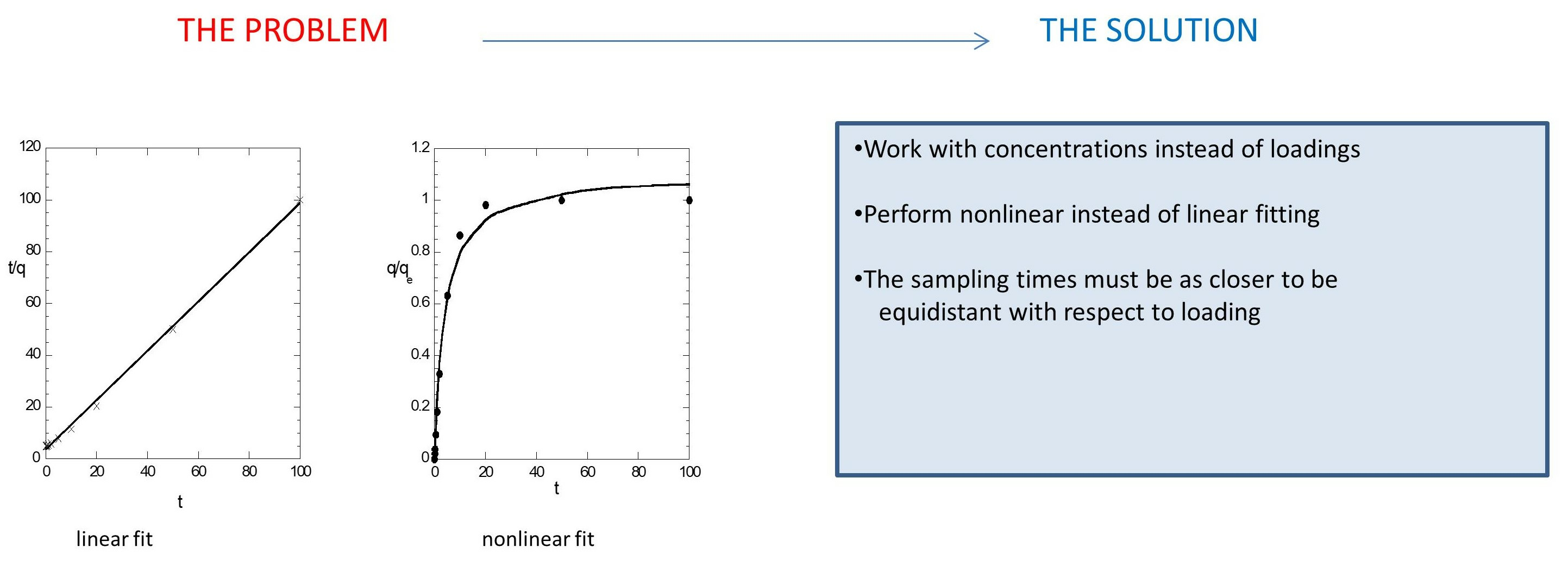
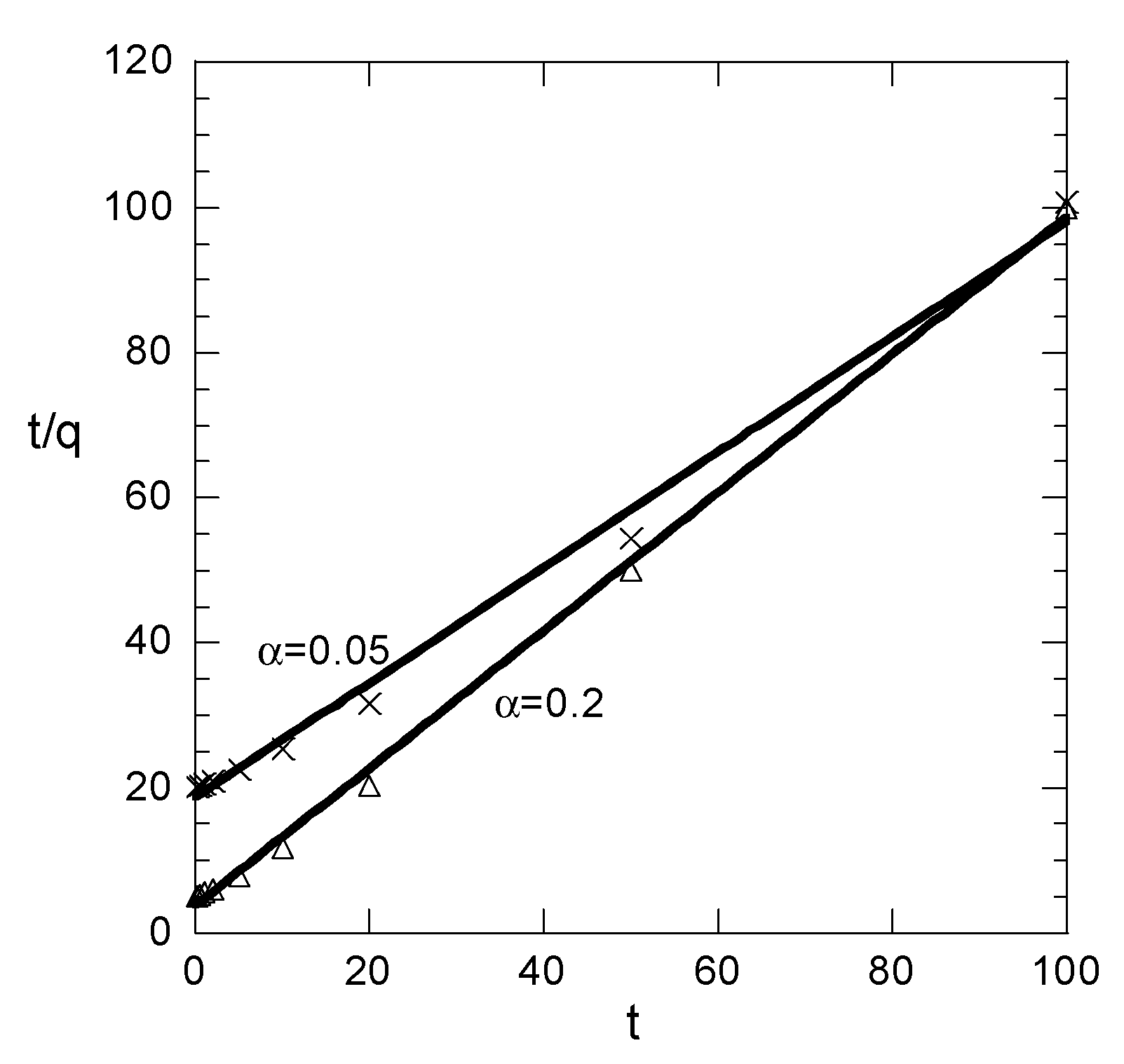
In order to have a further view of what the above values mean for fitting quality, the experimental values of q appear as symbols and the nonlinear fit (i) as continuous curves in Figure 1. The results for each value of α appear in different subfigure just for clarity because the attempt to show everything in a simple figure led to absolute confusion. In addition, the t/q data and their linear fit appear in Figure 2 for the two smaller values of α. The results for the other two values are not shown because the data are fitted perfectly by the straight line.

In case of small values of α, all three correlation coefficients imply good fitting. The linear fitting values R₂² and R₃² are smaller than the nonlinear fitting one R₁². This is normal behavior; however, it is associated only with the sampling times accumulated at the fast increasing part of the q curve. Such a situation is not typically encountered in the literature. As sampling times begin to be distributed to the slowly increasing part of the q data, the situation is radically changed. The R₁² decreases (taking values indicating successful fitting up to α = 0.5) as α increases. However, the linear fitting correlation R₂² appears to increase with α, implying a perfect fit for α > 0.2. This is certainly misleading, given that the correlation coefficient R₃², representing the real quality of the linear fitting, is very low, denoting poor fitting for α > 0.2.

Summarizing the above, the findings are: As the sampling times are distributed at larger ranges of q, the linear fitting of t/q data appears to be perfect and the corresponding correlation coefficient (R₂²) is larger than the one (R₁²) of nonlinear fit of q data. However the q vs. t correlation based on linear fitting appears to be very poor. In practice, the sampling times usually cover an extensive range of q, implying that the linear fit procedure always suggests a perfect success of the pseudo-second order kinetic model (even if the data exactly follow the pseudo-first order kinetics). However the success of the linear fitting is fake; it is simply an outcome of the data transformation. The parameters resulting from the linear fitting procedure lead to a very poor direct correlation between q and t. These arguments are not quite new, since they have been proposed by other researchers in recent years [1,33,34]. However it appears that most researchers are not convinced, so additional work is needed in this direction.

2.2. Example 2

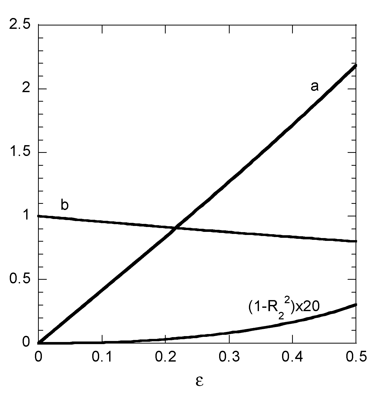
The second example is a more extreme one, and reveals how much fake the linear fitting approach can be. Let us assume four sampling times: 2, 5, 10, and 50, at which the value of q is unity. Obviously there should not be any kinetic model derived from these data. A random noise is added to these data so that q = 1 + ε (rnd − 0.5). The parameter ε is the amplitude of the noise and the variable rnd denotes a random number uniformly deviating between 0 and 1. The specific rnd values 0.8, 0.3, 0, and 0.9 have been used for the following numerical data. It is noted that the attempt to perform the nonlinear fit (case (i) above) leads to a complete failure (close to zero or negative value for R₁²). This behavior is expected, and appears to be correct since no kinetic information actually exists for the particular q data. However when an attempt is made to fit the data by the linear fitting model (ii), the resulting R₂² indicates complete success. The parameters a and b resulting from the linear fitting procedure appear as a function of the noise amplitude ε in Figure 3. The correlation coefficient is presented as (1 − R₂²) × 20 in order to enhance the resolution of the presentation. The fitted value of b is relatively stable to noise (decreased by 20%) as ε increases from 0 to 0.5. This is not the case for parameter a which increases from 0 to 2.18 under the same circumstances denoting an unstable to noise behavior. However regardless of the stability of the results, the key point is that a successful linear fit appears in all cases (R₂² is 0.985 even for ε = 0.5). The above example is a clear indication that employing linearized edition of the pseudo-second order model leads to fake successful fits, even when using data with no information for the kinetic behavior of the process.

2.3. Example 3

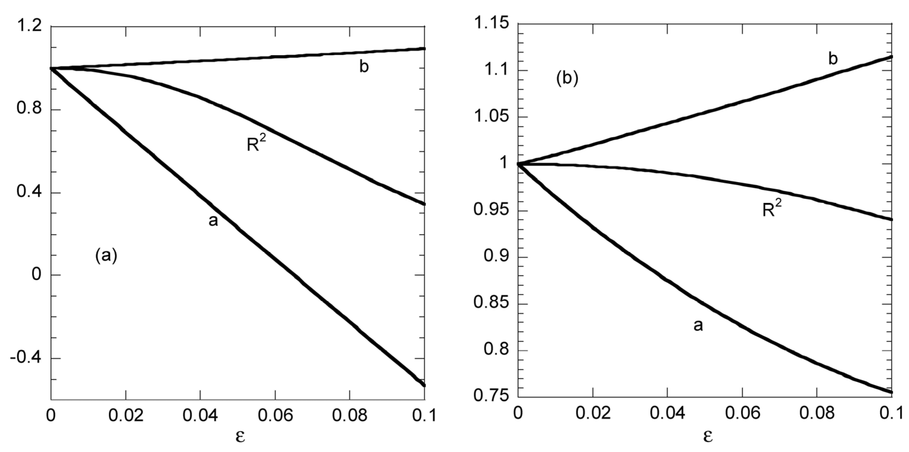
In this example, the effect of the distribution of sampling points in time is examined. The primary data are assumed to follow the pseudo-second order equation q = t/(1 + t) (i.e., a = b = 1). The first case (Case 1) corresponds to bad sampling strategy and contains the sampling times t = 2, 5, 10, 20, 50, and 100. In this case the difference in q between two consecutive sampling points is highly non-uniform. The second case (Case 2) corresponds to what was found to be the optimum sampling strategy for which two consecutive sampling points have the same difference in q. After the calculation of “experimental” q values, they are polluted using a staggering experimental error altering between +ε and −ε for consecutive sampling points. This procedure is an alternative way to examine the fitting stability with respect to the random noise used in the previous example. Both nonlinear and linear fitting procedures are applied to the data constructed in the above ways, and the parameters a and b are estimated for several values of the artificial experimental error parameter ε. It is noted that the symbol R² designates the difference between the non-linear fitting arising q values and the nominal ones (before addition of the “experimental” error). The scope of this choice is to present the distance between fitted and “exact” values of q. If R₁² is used instead of R² the general picture presented in the following would not be different. The values of R₁² are slightly larger than those of R² for Case 1 data, whereas R₁² and R² are exactly the same for Case 2 data.

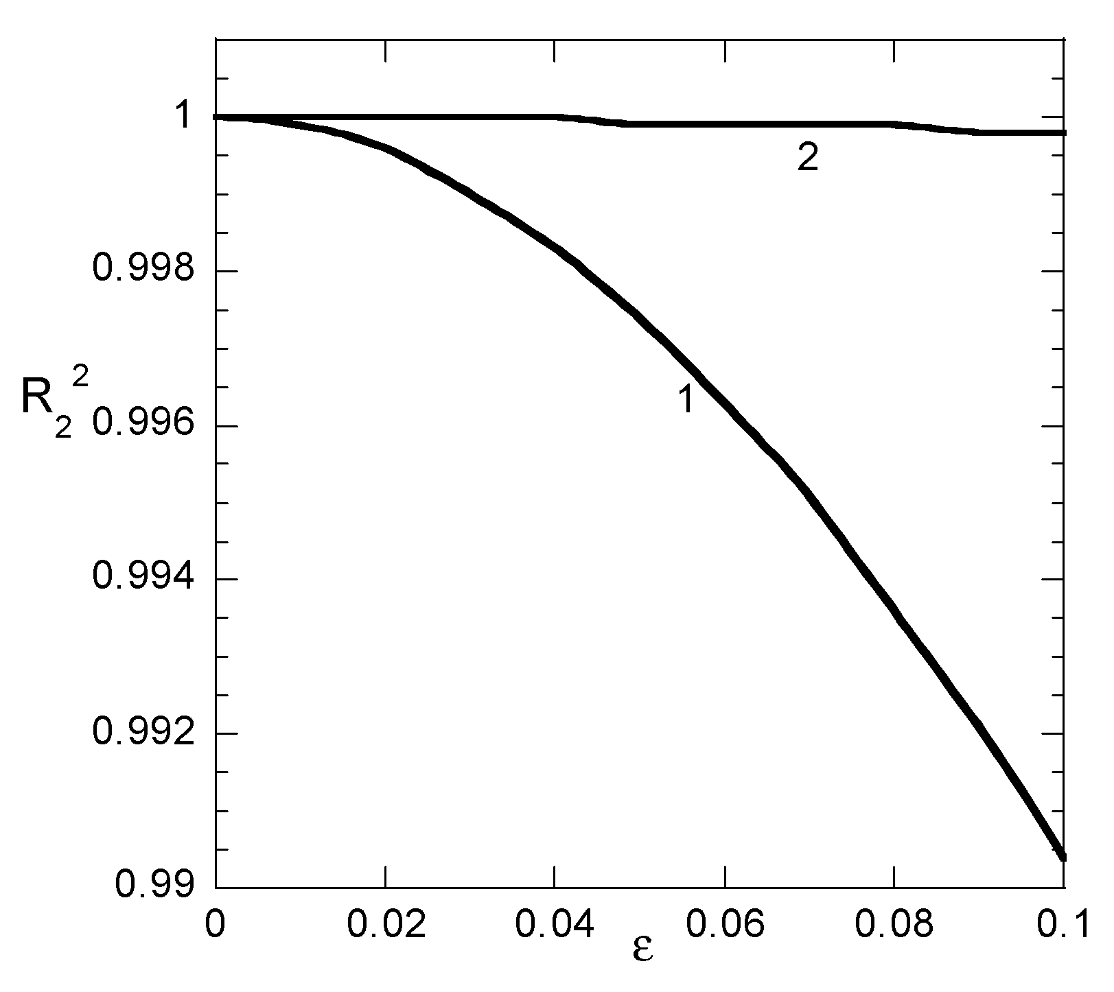
The values of a and b resulting from linear fitting procedure and the values of R² for non-linear fitting appear, versus the “experimental error” parameter ε in Figure 4a,b for Case 1 and Case 2 data, respectively. The corresponding values R₂² for linear fitting appear separately in Figure 5 since a different y-axis scale is required for them. Let us start to discuss Figure 4 from the evolution of R² of the nonlinear fitting. Obviously, the sampling time distribution plays a crucial role in the fitting quality. The R² for Case 1 data decreases to 0.965 at ε = 0.02 whereas the same value is reached for Case 2 data at ε = 0.08. This means that the proper distribution of sampling times stabilizes the nonlinear fitting procedure with respect to experimental error. Regarding linear fitting, it can be noticed that there is some stability with respect to parameter “b” values for both Case 1 and Case 2 data. The error in its derivation does not exceed 10% even for ε = 0.1. On the other hand, the linear fitting procedure is quite unstable with respect to parameter “a” in Case 1 data (the error is already 15% at ε = 0.01) whereas a poor stability appears for Case 2 data (error 25% at ε = 0.1). However, the data presented in Figure 5 suggest that the linear fitting appears to be always perfect (R₂² larger than 0.9998) for Case 2 data or very good (R₂² larger than 0.99) for Case 1 data. Once again, it is shown explicitly that the linear fitting procedure leads to misleading results. The additional information acquired by Example 3 shows that the sampling time distribution is crucial for the quality of the nonlinear fitting. The more equidistant in q the sampling times, the more accurate the fitting.

The reason for the phenomenal success of the linear pseudo-second order model is that the second term of the right hand side of Equation (6) is getting over-weighted with respect to the first term as time increases. This leads to a small sensitivity with respect to k₂ and to a fitting which almost entirely depends on q_e. Such a situation cannot be observed in the linearization of the pseudo-first order kinetic model.

3. Further Discussion

Another important issue is the extensive use of q as the dependent variable for the kinetic modeling in literature. However, q is not a directly measured quantity but rather is calculated from the measured concentration C as q = V(C_o − C)/m. Substituting the above relation in the pseudo-second order kinetics equation leads to the following form (where C_e = C_o − mq_e/V):

$$\frac{\mathrm{d}\mathrm{C}}{\mathrm{d}\mathrm{t}}=-\frac{\mathrm{V}{\mathrm{k}}_2}{\mathrm{m}}{(\mathrm{C}-{\mathrm{C}}_{\mathrm{e}})}^2$$

(10)

introducing the new variable c = C/C_o and integrating the above equation leads to the form:

$$\mathrm{c}=\mathrm{B}+{(\frac{1}{1-\mathrm{B}}+\mathrm{A}\mathrm{t})}^{-1}$$

(11)

where B = C_e/C_o and A = Vk₂C_o/m. There are several reasons for which Equation (11) must be used for the fitting of the pseudo-second order model instead of Equation (5). At first, any uncertainty for the variables m and V are transferred to the data for q, so it is not easy to estimate its effect on the evaluated parameters q_e and k₂. On the other hand, using Equation (11), the C data depend only on concentration measurements and the uncertainty in m; V appears only in the dimensionless parameter A, rendering trivial the assessment of its impact in k₂ evaluation. The second point is that for a specific measurement, uncertainty in concentration of the relative C error is small in regions where the relative q error is large. This inverse behavior of relative error is undesirable, since the q error is a calculated and not a measured one. Finally, according to Example 1, the sampling time must be accumulated at the initial part of the q curve. However, in this region the relative error in q is large (compared to the one in C), which jeopardizes the quality of the fitting procedure. It is noted that the pathology described above for fitting of q with the linear form of the second order model does not exist for fitting of the c curve in a linear form. This is why the above pathology has not been identified in Chemical Reaction Engineering literature [35] for fitting data of second order reactions (i.e., reactant concentration data are always employed). However, in any case, the non-linear fitting is preferable. All analysis of the present work is based on the minimization of the sum of the square deviation as fitting criterion. There are of course several alternative criteria to perform the fitting procedure [36]. However. the use of any criterion would not change the general picture created by the examples presented above.

After the completion of the present study, the work of Simonin [1], which shares some common issues with the present work, came to our attention. The pseudo-first and pseudo-second order models are examined using procedures similar to the present ones (first order data, noise addition) and a bias of the second order over the first order model was found (the explanation is similar to the one proposed here). The nonlinear fitting procedure and the use of points far from the equilibrium are also suggested. However, despite the large number of literature references to [1] our experience as reviewer suggests that the majority of researchers continue to use the linear version of the pseudo-second order model to fit their data. In fact, reference [26], which proposes the pseudo-second order model, has almost ten times more citations than [1] during the last six years. Some recent works employing the linear version of the pseudo-second order method and finding excellent fitting can be found in the reference list [37,38,39,40,41]. The reference [26] has a total of 16,000 citations. A random sampling for 100 of them led to 94 works that find an excellent fit of the linear version of pseudo-second order model to their data. One can imagine what the actual number of works following the particular approach. Over the past few years, several authors have suggested the researchers to avoid this particular model, but the response appears poor. This means that further attempt must be made to convince the researchers to avoid incorrect use of pseudo-second order model and the present work supports this target.

The present work must be read in conjunction with [1] since it offers further support to its arguments. The additional information in the present work is (I) the fake success of the pseudo-second order model could make it appear better even than sophisticated mechanistic models. (II) It is better to make the fitting on evolution of variable C (directly measured quantity) instead on evolution of q. (III) for a given number of experimental points, as the results improve the more equidistant the points in C domain become.

4. Conclusions

The detailed analysis and the examples presented make clear that the success of linear edition of the pseudo-second order kinetic model in describing experimental adsorption kinetics is an artificial one and it is based on overweighting of the large t behavior of the q data through a rearrangement for their description by a straight line. The presented examples also lead to the following suggestions for the correct treatment of the adsorption kinetic data in respect to their fitting by the pseudo-second order kinetic model: (I) It is preferable to work with a directly measured quantity such as solute concentration (C) instead of the calculated quantity of adsorbed mass of solute (q). (II) The use of non-linear fitting instead of linear fitting is strongly recommended. (III) The best possible distribution in time of the experimental data points is the one with data points that have the same distance to each other in the C value. It is not always easy to achieve this in practice, but any improvement of the data distribution in this direction also improves the fitting procedure quality. The above suggestions holds not only for the pseudo-second order model but for any model used to fit the data (including even sophisticated phenomenological models). However, they are quite essential for the use of the second order model, since they ensure that an artificially excellent fit to the data will not emerge.