Communication

Interfacial Dilational Viscoelasticity of Adsorption Layers at the Hydrocarbon/Water Interface: The Fractional Maxwell Model

1
Institute of Condensed Matter Chemistry and Technologies for Energy, Unit of Genoa, 16149 Genoa, Italy
2
Institute of Biocolloid Chemistry, 03142 Kyiv (Kiev), Ukraine
3
Department of Colloid Chemistry, St. Petersburg State University, 198504 St. Petersburg, Russia
4
Max Planck Institute of Colloids and Interfaces, 14424 Potsdam/Golm, Germany
*
Author to whom correspondence should be addressed.
Colloids Interfaces 2019, 3(4), 66; https://doi.org/10.3390/colloids3040066
Submission received: 13 November 2019 / Revised: 5 December 2019 / Accepted: 6 December 2019 / Published: 10 December 2019
(This article belongs to the Special Issue B&D 2019)

Abstract

:
In this communication, the single element version of the fractional Maxwell model (single-FMM or Scott–Blair model) is adopted to quantify the observed behavior of the linear interfacial dilational viscoelasticity. This mathematical tool is applied to the results obtained by capillary pressure experiments under low-gravity conditions aboard the International Space Station, for adsorption layers at the hydrocarbon/water interface. Two specific experimental sets of steady-state harmonic oscillations of interfacial area are reported, respectively: a drop of pure water into a Span-80 surfactant/paraffin-oil matrix and a pure n-hexane drop into a C13DMPO/TTAB mixed surfactants/aqueous-solution matrix. The fractional constitutive single-FMM is demonstrated to embrace the standard Maxwell model (MM) and the Lucassen–van-den-Tempel model (L–vdT), as particular cases. The single-FMM adequately fits the Span-80/paraffin-oil observed results, correctly predicting the frequency dependence of the complex viscoelastic modulus and the inherent phase-shift angle. In contrast, the single-FMM appears as a scarcely adequate tool to fit the observed behavior of the mixed-adsorption surfactants for the C13DMPO/TTAB/aqueous solution matrix (despite the single-FMM satisfactorily comparing to the phenomenology of the sole complex viscoelastic modulus). Further speculations are envisaged in order to devise combined FMM as rational guidance to interpret the properties and the interfacial structure of complex mixed surfactant adsorption systems.

1. Introduction

A large variety of natural materials and industrial products exhibit a viscoelastic behavior when subjected to periodic or transient stress-strain perturbations, responding to the imposed perturbations with typical frequency spectra or evolving along peculiar time scales [1].
The viscoelastic properties are often phenomenologically modelled by a spring and a dashpot in series (Maxwell model) or in parallel (Kelvin–Voigt model), as well as by complex assemblages of these two elements [1,2,3,4].
In recent years, the fractional Maxwell model (FMM) was fruitfully adopted for analysing the 3D-viscoelastic behavior for several classes of bulk materials, in particular for soft materials, by using only a few constitutive parameters and still retaining a good corresponding agreement between model values and the observed experimental results [5,6,7,8,9,10,11,12,13]. Lei et al. [14] and Stankiewicz [15] reviewed various scientific and technological fields of successful FMM applications. Povstenko expounded the mathematical foundations of the inherent fractional-derivative tool [16].
Jaishankar et al. introduced the FMM in the particular study of interfacial shear and dilational viscoelasticity, pointing out its adequacy for the description of bulk viscoelastic materials as well as complex interfacial viscoelasticity [17,18]. Specifically Sharma et al. suggested the possible coupling of bulk and interfacial viscoelasticity in case of particular soft matters, where the interfacial contribution is eventually significant to the 3D-viscoelasticity results [19].
In this communication, we report the application of the single element FMM to the interfacial dilational viscoelastic results, obtained by capillary pressure experiments under low-gravity conditions aboard the International Space Station, for adsorption layers at the hydrocarbon/water interface. The experiments with single water-in-oil and oil-in-water drops are important for deeper understanding the fundamental laws governing the dynamic behavior of adsorption layers occurring in real emulsions.

2. Materials and Method

2.1. Materials

A set of two experimental systems was studied. The constituting materials for the first system were: (a) MilliQ pure water, (b) Fluka paraffin-oil, (CAS 8012-95-1) and (c) sorbitan monooleate (Span-80), (CAS 1338-43-8). The second system was constituted by (a) MilliQ pure water, (b) n-Hexane for spectroscopy Uvasol®, (CAS 110-54-3), (c) tridecyl dimethyl phosphine oxide (C13DMPO), (CAS 186953-53-7) and (d) tetradecyl trimethyl ammonium bromide (TTAB), (CAS 1119-97-7).
The composition of the studied couple of two-phase liquid systems was described in full details in [20,21].

2.2. Apparatus

The low-gravity experiments were conducted aboard the International Space Station (ISS) by an especially devised facility, denoted as FASTER (Facility for Adsorption and Surface Tension Research). The apparatus included two experiment cells, respectively operating on the above-mentioned experimental systems. The first cell was dedicated to the study of the dynamic interfacial properties of a pure-water (spherical-cap shaped) drop, generated inside a Span-80/paraffin-oil matrix, while in the second cell a pure-hexane (spherical-cap shaped) drop was generated inside an aqueous C13DMPO/TTAB mixed solution matrix. Typical video frames of the drops inside the liquid matrices were, for example, visualized in Figure 4 of [20] and in Figure 1 of [21].

2.3. Experimental Procedure

A piezo-actuator, built in the measurement cell, allowed the harmonic oscillations of the drop interfacial area to be excited at 8 different frequencies (0.01, 0.02, 0.04, 0.08, 0.16, 0.32, 0.5, and 1.0 Hz), 3 different relative-area amplitudes (5%, 10%, and 20%), 3 different temperatures (first cell T = 20, 30, and 40 °C, second cell T = 15, 20, and 30 °C) and various different matrix concentrations. Telemetered data management, calibration and capillary-pressure measurement procedures were explicated in [20,21].
In all experiments the achievements of linearity in a rheological ground state was an important concern. To this end, the starting time for the incipient 8-frequency-/5%-amplitude-oscillation sequence was established at t = 2500 s after the drop generation inside the liquid matrix. Such time interval appeared sufficient to reach the steady-state equilibration (i.e., the rheological ground state) of the interfacial layer.
Figure 1, illustrating an example for the smallest surfactant concentration of the second experimental system (i.e., C13DMPO/TTAB adsorbed at water/hexane interface), shows that the mean-level values of interfacial tension, γ, as a function of frequency, is constant for all amplitudes (but random disturbances inherent in the intermittent piezo push-pull action), albeit γ attains a somewhat smaller level for the final 20%-amplitude oscillation sequence.
Moreover, Figure 1 shows the interfacial dilational viscoelasticity behavior, as a function of frequency, determined by Fourier series expansion analysis. Inspection of the data for 5%-, 10%-, 20%-amplitudes, indicates an acceptable linearity condition of the interfacial γ-responses (and the measurement repeatability, as well).
The results for the first experimental system (i.e., Span-80 adsorbed at paraffin–oil/water interface) revealed the same trends: almost constant mean-level values of interfacial tension and an acceptable linearity range for the interfacial responses to area perturbations up to 20% amplitude (cf. Figures 13, 14, and 17 in [20]).

3. Brief Outline of the Applied Model

3.1. The Interfacial Dilational Viscoelastic Modulus

The interfacial dilational viscoelastic modulus, ε*(iω) is a physical quantity defined in the frequency domain by a complex expression [22]:
ε * ( i ω ) = ε r ( ω ) + i ε i ( ω ) = Δ γ × exp [ i ( ω t + ϕ ) ] Δ A × exp ( i ω t ) / A 0 ,
where ω represents the angular frequency, Δγ × exp[−i(ωt + ϕ)] is the interface response to the imposed area perturbation ΔA × exp(−iωt)/A0, Δγ and ΔA are the oscillation amplitudes of the interfacial tension and the interfacial area, respectively, ϕ the phase shift between perturbation and response, A0 is the mean interfacial area of the sinusoidal cycle, ε r and ε i are the real and imaginary parts, respectively, of the complex viscoelasticity ε*(iω).
The definition of ε*(iω) in Equation (1) is extended by the existence of a Fourier transform relationship between the three physical quantities involved in interfacial extension/contraction processes, that is, fractional-area change (time domain), interfacial tension change (time domain) and interfacial dilational modulus (frequency domain) [23]:
ε * ( i ω ) = ε r ( ω ) + i ε i ( ω ) = F { Δ γ ( t ) } F { Δ A ( t ) / A 0 } ,
where F is the Fourier transform operator.
The definition of ε*(iω) according to Equations (1) and (2), does not require any assumption about the microscopic structure of the studied interface or about the molecular mechanisms occurring in the interfacial layer or in its immediate proximity. The only implicit assumption in Equations (1) and (2) is that the interface behaves as a time-invariant linear system, i.e., that the interface is in adsorption equilibrium condition and it is subjected to small amplitude perturbations.
It is worth noting that the physical quantity ε*(iω) is a constitutive property of the interfacial systems, taking a definite value at each particular frequency. Actually, ε*(iω) can be conceived as the transfer function of the interfacial system, connecting the interfacial Δγ responses to interfacial area perturbations of any functional form in the frequency–domain or in the time–domain. In other words, the definition of ε*(iω) can be expressed in terms of the Δγ response to the unit-step function u(t).
Specifically, for a unit-step strain (ε(t) ≡ ΔA(t)/ΔA = u(t)) input of interfacial-area extension/contraction, the Fourier transformation in Equation (2) leads to the following integral expression for the output interfacial tension stress:
ε * ( i ω ) = i ω Δ A / A 0 × 0 Δ γ ( t ) × e i ω t d t .
Hence, applying the Euler identity, the values of the real and the imaginary part of ε*(iω) can be interpreted as the integration values of the Δγ(t) relaxation function excited by a unit step change of fractional area [24]:
ε * ( i ω ) = i ω × F { Δ n γ ( t ) } = ω 0 Δ γ n ( t ) sin ( ω t ) d t + i ω 0 Δ γ n ( t ) cos ( ω t ) d t
where the relaxation function is normalized by the relative area change, Δγn(t) = Δγ(t)/(ΔA/A0).
The expression of Equation (4), as for the case of Equation (2), is valid whatever the mechanism at the molecular level is, which generates the observable interfacial viscoelasticity phenomenology.
The definition of ε*(iω) in Equations (1), (2), and (4) still holds in non-ideal initial adsorption equilibrium provided that the Δγn(t) relaxation function vanishes at zero value in a time interval at least one order of magnitude shorter than the time-interval of the non-equilibrium condition evolution, at the start of the interfacial layer excitation.

3.2. Maxwell Model

The classic Maxwell viscoelastic model is constituted by the arrangement in series of a linear elastic (Hookean) spring and a linear viscous (Newtonian) dash-pot, with parameters E (Young’s modulus) and η (coefficient of viscosity), respectively.
The constitutive equation of a (single-element consisting of one spring and one dash-pot) Maxwell model requires equilibrium between stress, σ, and strain, ε, according to the following equality [5,15]:
E η × σ ( t ) + d σ ( t ) d t = E × d ε ( t ) d t .
For a unit-step strain input, ε(t) = u(t) (Heaviside step function), at time t ≥ 0 the induced output stress follows an exponential relaxation function:
σ ( t ) = E × e t τ ,
where τ = η/Ε is the characteristic relaxation time.
For the application of the Maxwell model to the interfacial dilational viscoelasticity, the notations of Equation (6) are appropriately modified as:
Δ γ ( t ) = ( Δ A / A 0 ) Δ γ n ( 0 ) × e t τ
where Δγn(0) is the interfacial tension value at time t = 0 s for Δγn(t) = Δγ(t)/(ΔA/A0).
Hence, the insertion of Equation (7) in Equation (4) takes the form:
ε * ( i ω ) = ω 0 Δ γ n ( 0 ) e t τ × sin ( ω t ) d t + i ω 0 Δ γ n ( 0 ) e t τ × cos ( ω t ) d t
Upon integration of Equation (8), the real part of the complex modulus reads:
ε r = Δ γ n ( 0 ) × ω 2 ( 1 / τ ) 2 + ω 2 = Δ γ n ( 0 ) × τ 2 ω 2 1 + τ 2 ω 2
and the imaginary part reads:
ε i = Δ γ n ( 0 ) × ω × ( 1 / τ ) ( 1 / τ ) 2 + ω 2 = Δ γ n ( 0 ) × τ ω 1 + τ 2 ω 2
After algebraic operations, from Equations (9) and (10) the expression for the modulus of the complex function of viscoelastic modulus for the single element Maxwell model can be obtained as follows:
| ε * ( i ω ) | = Δ γ n ( 0 ) × τ ω 1 + τ 2 ω 2

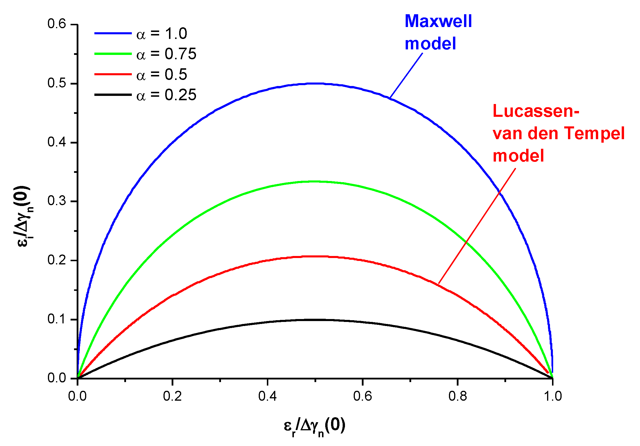
3.3. Fractional Maxwell Model

The generalised Maxwell model is constituted by a summation of Maxwell single elements, representing the behavior of a parallel sequence of Maxwell spring/dash-pots.
| ε * ( i ω ) | = i = 1 n Δ γ n ( 0 ) × τ ω 1 + τ 2 ω 2
Such a generalised Maxwell model usually requires multiple exponential functions to calculate the relaxation time-spectra for complex soft materials. An alternative approach can be built on employment of the fractional Scott–Blair model. The fractional Scott–Blair element is defined by the following fractional differential equation [5,10,15]:
σ ( t ) = E τ α × d α ε ( t ) d t α
where τ = η/E is a characteristic time scale, α is a dimensionless positive non-integer number (0 < α < 1), assigning the order of the fractional derivative of the strain ε(t) (known as Caputo fractional derivative). This mathematical tool, represented as a ladder sequence of Maxwell spring/dash-pots, allows combining a range of multiple exponential relaxation mechanisms in a single three-parameter rheological element (see [15] for mathematical details and graphical representation).
In the present study, we will consider a fractional single Maxwell element, which consists of a fractional Scott–Blair element, defined by Equation (13) with the parameters E1, τ1, and α, and a spring, E2, connected in a series. The constitutive equation for this model is given by [11,15]:
E τ α d α ε ( t ) d t α = σ ( t ) + τ α d α σ ( t ) d t α ,
where E = E2 and τ α = ( E 1 / E 2 ) × τ 1 α
Upon similar operations as described in Equations (7)–(11) for the single-element Maxwell model, the proper Fourier transformation for the unit-step strain (i.e., specifically, the unit-step change of relative interfacial area) leads to the following expressions for the surfactant adsorption layers, namely, the real and imaginary parts of the complex interfacial dilational viscoelastic modulus (see [11] for mathematical details):
ε r = Δ γ n ( 0 ) × ( τ ω ) 2 α + ( τ ω ) α cos ( π α / 2 ) 1 + ( τ ω ) 2 α + 2 ( τ ω ) α cos ( π α / 2 ) ,
ε i = Δ γ n ( 0 ) × ( τ ω ) α sin ( π α / 2 ) 1 + ( τ ω ) 2 α + 2 ( τ ω ) α cos ( π α / 2 ) .
Finally, embodying just three parameters E = Δγn(0), τ and α, the determined modulus of the complex function ε*(iω) for a single-element fractional Maxwell model reads:
| ε * ( i ω ) | = Δ γ n ( 0 ) × ( τ ω ) α 1 + ( τ ω ) 2 α + 2 ( τ ω ) α cos ( π α / 2 ) .

3.4. Lucassen–van den Tempel Model

For a diffusion-limited adsorption mechanism the dynamic dilational viscoelasticity modulus of the adsorption layer is described by the well-known Lucassen–van den Tempel model [22]:
ε r = Δ γ n ( 0 ) × 1 + ω D / ω 1 + 2 ω D / ω + 2 ω D / ω ,
ε i = Δ γ n ( 0 ) × ω D / ω 1 + 2 ω D / ω + 2 ω D / ω ,
where ωD is the characteristic frequency of diffusional relaxation.
It is interesting to see that the standard Maxwell model and the Lucassen–van den Tempel model are particular cases of the more general single-element fractional Maxwell model, described by Equations (15)–(17), for the parameter α = 1 and 1/2, respectively. This can be well seen in the Cole–Cole plots showing the imaginary part of the complex viscoelasticity as a function of the real part (Figure 2).
This figure shows that by varying the parameter α we have a continuous transition between different models. In particular, for the Lucassen–van den Tempel model we have α = 1/2, ωD = (2τ)-1 and ε0 = Δγn(0), which corresponds to a purely diffusional relaxation. In contrast, the case of α = 1 (i.e., the standard Maxwell model) corresponds to a purely kinetic controlled adsorption, as can be concluded from Figure 8.2 in [25]. Note, however, in the case of a mixed adsorption kinetics (diffusion complicated by an adsorption barrier) the single-element fractional Maxwell model cannot be applied as this case requires two different relaxation times for a proper description.

4. Results and Discussion

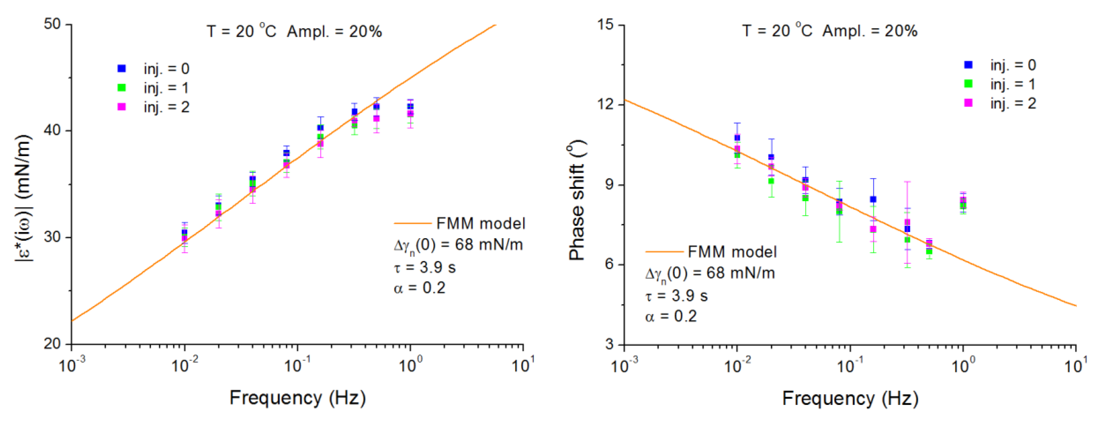
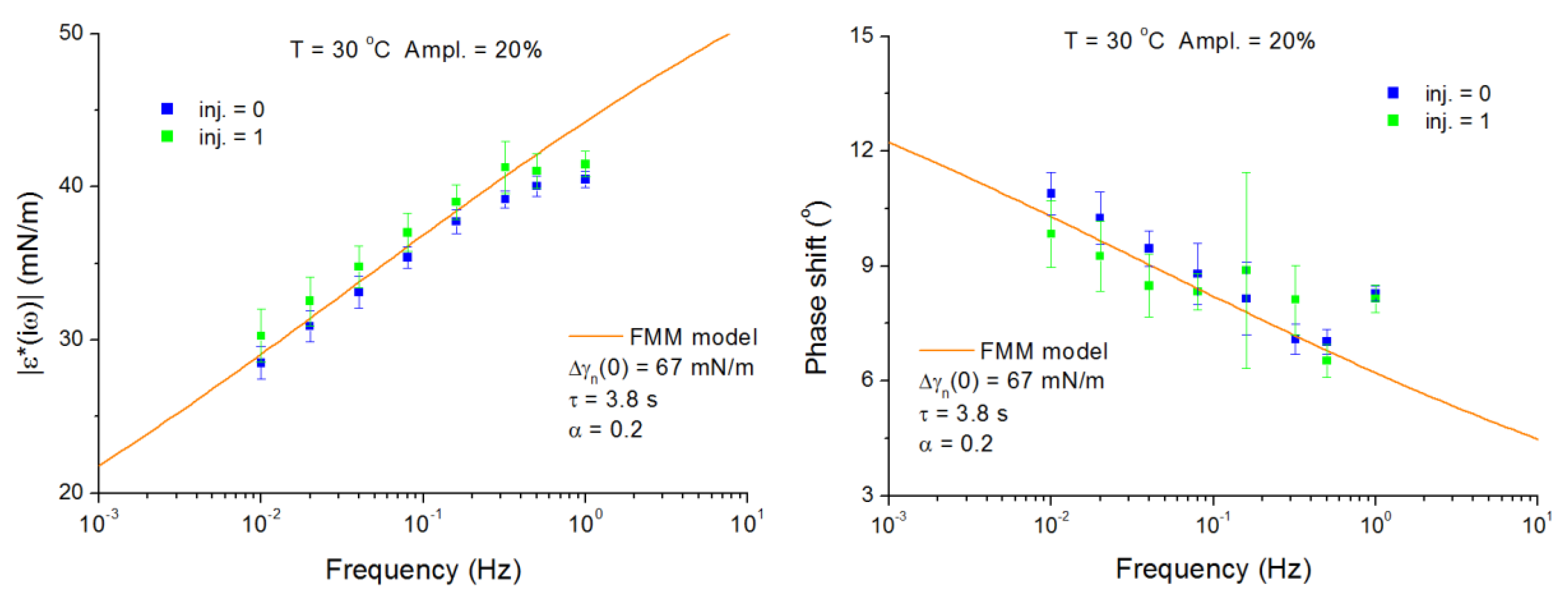
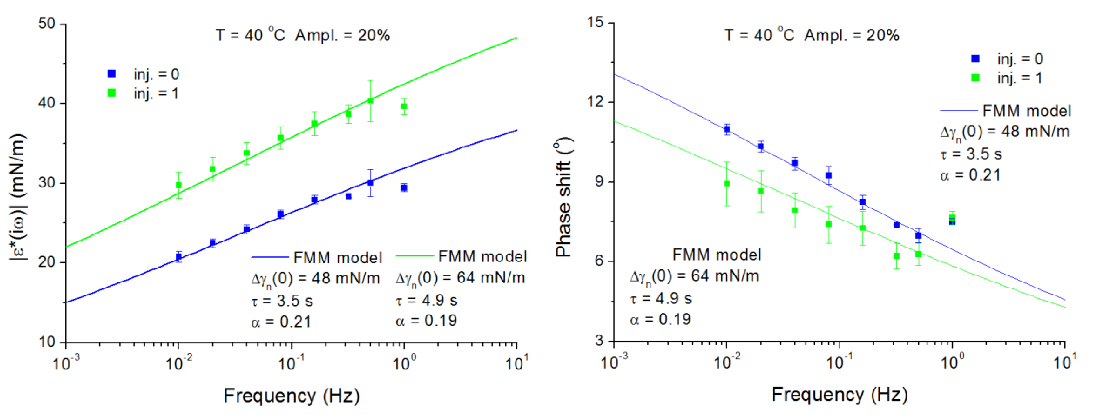
4.1. Span-80 Adsorption Layers at Paraffin–Oil/Water Interface

Figure 3, Figure 4, and Figure 5 show the experimental results for modulus | ε * ( i ω ) | and phase φ = a tan ( ε i / ε r ) of the complex viscoelasticity measured for Span-80 adsorbed at paraffin–oil/water interface at an amplitude of 20% and different temperatures. The results at other amplitudes (5% and 10%) are similar, but the relative experimental errors are the smallest for the amplitude of 20%. The experimental points in Figure 3, Figure 4, and Figure 5 are the averages of three different runs.
The experiments were planned for different concentrations of Span-80 in paraffin-oil created via a series of injections of small surfactant amounts into the matrix liquid. However, as it was reported before in [20], a leakage has occurred from the injection syringe during the facility upload and installation on the ISS. As a consequence, the value of real Span-80 concentration in the majority of experiments was approximately within the range c = 2.0 × 10⁻⁵–3.0 × 10⁻⁵mol/dm3, as it has been estimated from the measured mean level of γ(t)-value (γ0 = 23–26 mN/m) [20]. Therefore, the viscoelasticity modulus for all injections was approximately the same, as it is seen from Figure 3, Figure 4, and Figure 5. The exception are the results for the injection no. 0 (nominally pure paraffin-oil) at temperature 40 °C, shown in Figure 5. These results were obtained under conditions of incomplete mixing of surfactant after the leakage, while the concentration in the vicinity of the drop interface remained smaller and the interfacial tension remained higher—within the range γ0 = 31–33 mN/m (for more details see [20]). This particular experiment was the first in the time-line. All subsequent experiments were performed after stirring actions resulting in a more homogeneous surfactant distribution.
All experimental data shown in Figure 3, Figure 4, and Figure 5 demonstrate similar trends: the modulus is increasing, whereas the phase shift is decreasing with increasing frequency. These experimental data can be fitted by using the simplest (single-element) FMM model, as given by Equations (15)–(17), as it is seen from Figure 3, Figure 4, and Figure 5. The model allows fitting both the modulus and the phase shift simultaneously, with the same parameter sets shown in the figure panels. The parameters of the model vary not in wide limits—α is about 0.19 and 0.2, τ is about 3.8 and 4.9 s, and Δγn(0) is about 64 and 68 mN/m for most of the experiments. Only for the incipient experiment (injection no. 0 at temperature 40 °C) the parameters are slightly different—α = 0.21, τ = 3.5, and Δγn(0) = 48 mN/m.
There are only obvious deviations of the model from the experimental data at the higher frequencies (mainly for the frequency 1 Hz). Most probably, such deviations can appear due to the increasing contribution of hydrodynamic effects, which can lead to a change of the system behavior (e.g., due to deviations of the drop shape from ideal spherical shape or more complicated relaxation mechanism).
The three parameters of the FMM model affect the shape of the modulus and phase shift vs. frequency dependencies in a different way. In particular, the phase shift does not depend on the multiplier before the frequency dependent part (“Δγn(0)”) in Equations (15) and (16). From the remaining two parameters, only the parameter “α” influences the slope of the phase shift vs. frequency dependence, whereas the second one (“τ”) is responsible for the shift of the whole curve along the frequency axis and does not influence the slope. Therefore, it is very easy to obtain these two parameters using only the phase shift vs. frequency dependence. On the other hand, these two parameters should be the same for the modulus vs. frequency dependence. Thus, we can easily find the remaining third parameter (“Δγn(0)”) by fitting this dependence. If the quality of fitting is good, this can be a criterion that the model is applicable for the considered system. The uncertainty in the fitting parameters can arise only from large experimental errors. For example, the slope of the phase shift vs. frequency dependence can vary within certain limits because the phase shift obtained in different experimental runs is slightly different, as it is seen in Figure 3, Figure 4, and Figure 5.
The Lucassen–van den Tempel model does not fit these experimental data properly. It allows to fit with a good accuracy the modulus only, but it does not allow to fit the phase shift (these results are not shown here). For this model, the slope of the phase shift vs. frequency dependencies appears approximately two times larger than the experimental one, because the Lucassen–van den Tempel model (α = 0.5) predicts the small-frequency limit of the phase shift equal to 45°, whereas the FMM model with α = 0.2 gives a limit of about 20°, which is much more consistent with the experimental data.

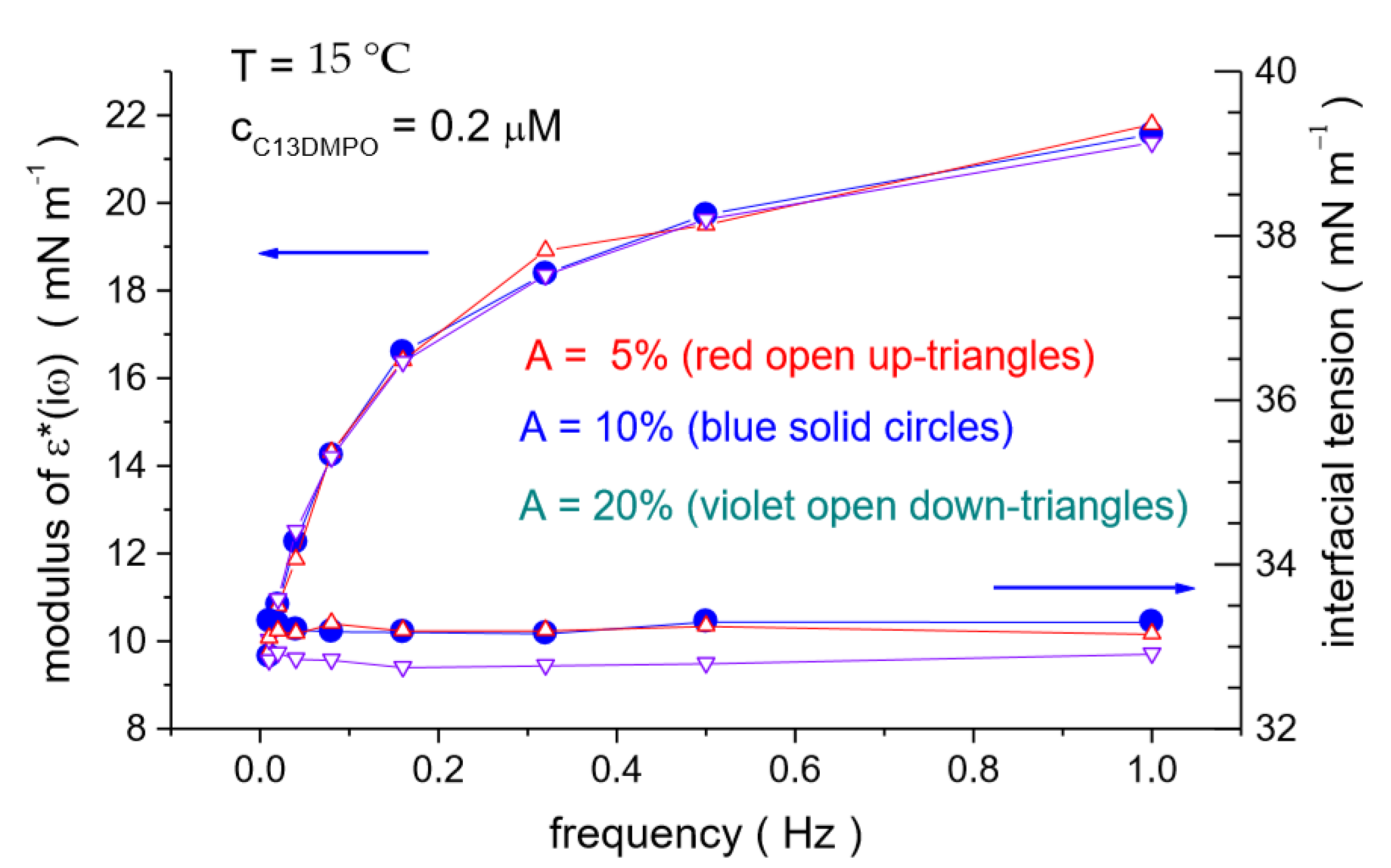
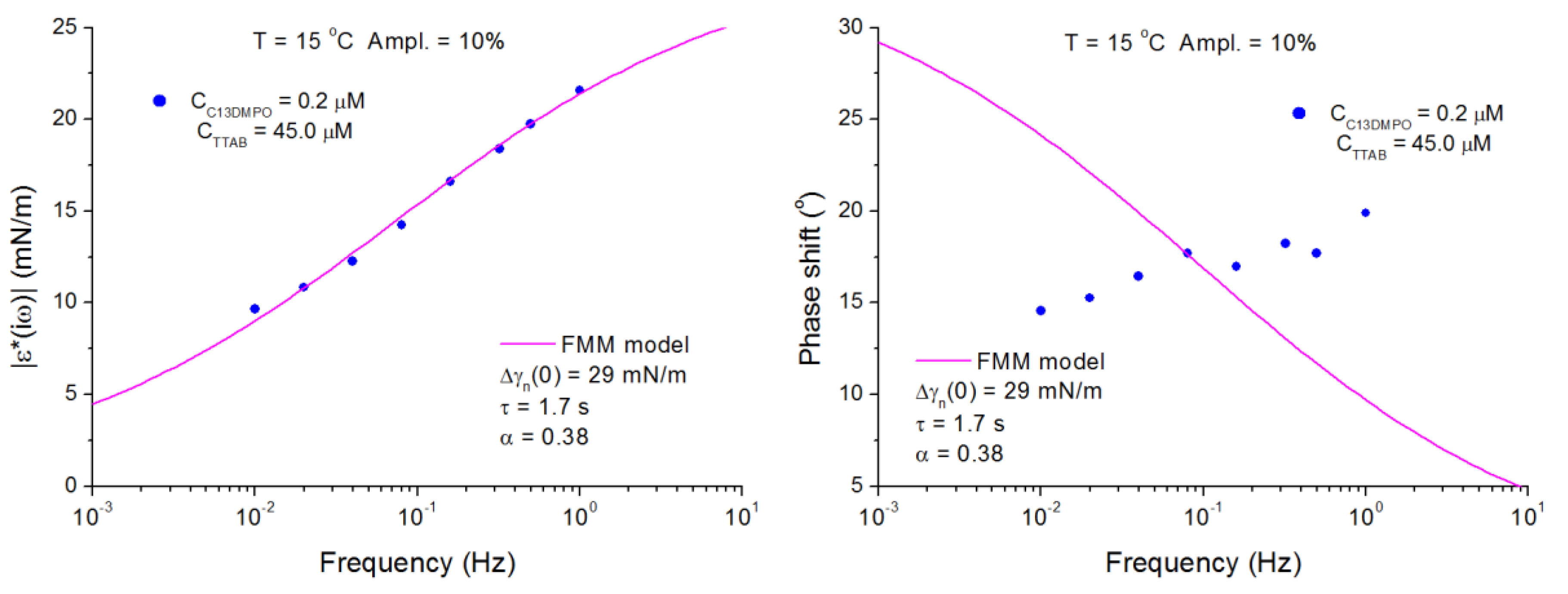
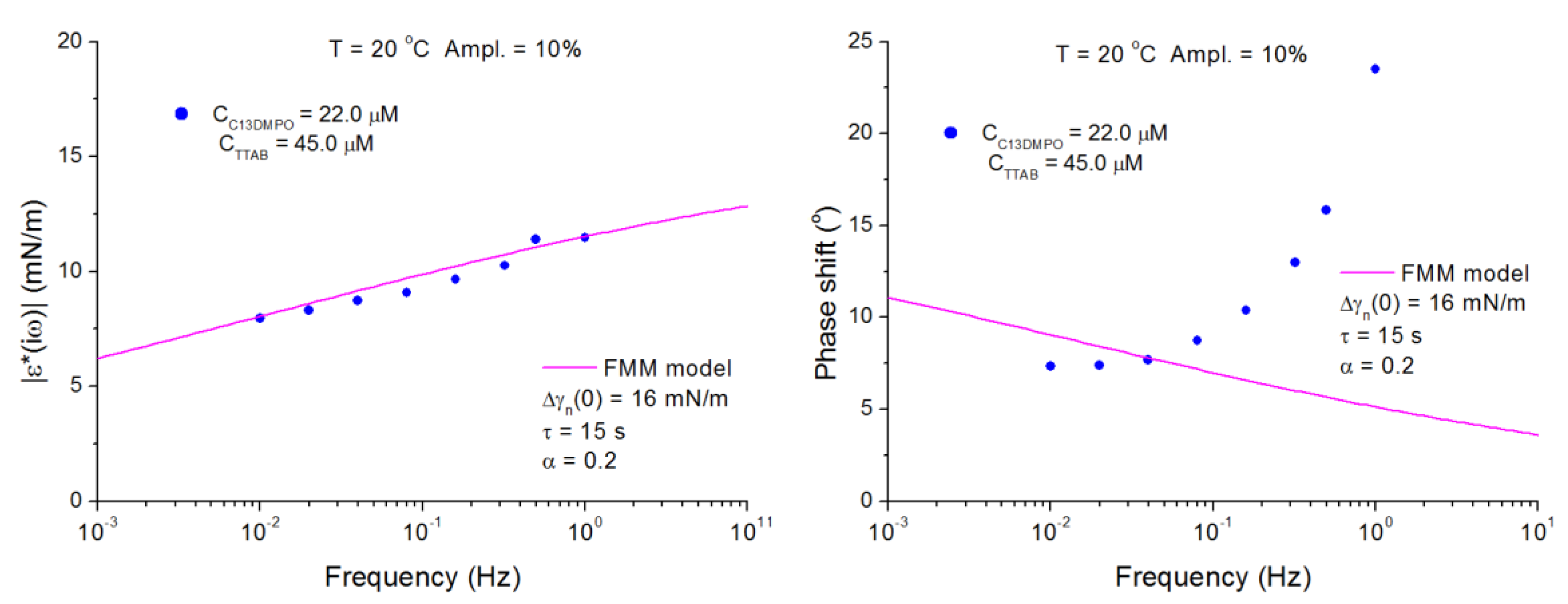
4.2. C13DMPO/TTAB Adsorption Layers at Water/Hexane Interface

The second set of experiments was performed with mixed C13DMPO/TTAB adsorption layers at water/hexane interface. The surfactants were injected by increasing small amounts into the aqueous matrix phase. The injected non-ionic C13DMPO has penetrated into the n-hexane drop, according to the partitioning equilibrium (its hexane-to-water distribution coefficient is about 30, [21,26]). The ionic TTAB does not dissolve in n-hexane and remained in the aqueous phase. Thus, if the interface is expanded or compressed, the equilibrium is restored due to TTAB adsorption/desorption from the aqueous phase and C13DMPO adsorption/desorption from both liquid phases. Two examples of the modulus and phase shift of the complex viscoelasticity vs. frequency dependencies for this system are shown in Figure 6 and Figure 7.
It is seen from these two examples that the single-element fractional Maxwell model allows fit to only the modulus and does not allow fit to the phase shift for the system considered here. This system is more complex as compared to that considered in the previous section, because it consists of two surfactants instead of one, while one of them is dissolved in both contacting liquids. Comparing the results in Figure 6 and Figure 7with those in Figure 3, Figure 4, and Figure 5 one can see that for mixed C13DMPO/TTAB adsorption layers at the water/hexane interface the phase shift is increasing with the frequency, while for Span-80 adsorbed at paraffin–oil/water interface it was decreasing. The single-element fractional Maxwell model predicts only a decreasing phase shift for all possible parameter sets. That is why this model does not fit the phase shift vs. frequency dependencies in Figure 6 and Figure 7. The classic Maxwell model and the Lucassen–van den Tempel model also predict only a decreasing phase shift as they are only particular cases of the fractional Maxwell model.
The analysis, presented in [21], has shown that there are two possible reasons for an increasing phase shift vs. frequency dependencies for mixed C13DMPO/TTAB adsorption layers at water/hexane interface. Such behavior can be explained by either the presence of a second surfactant in the system, or the effect of curvature of the drop interface (or a superposition of both effects). Thus, for many systems the rheological behavior of an adsorption layer similar to that in Figure 6 and Figure 7 is quite expected. For such systems, the single-element fractional Maxwell model is not sufficient and more complicated models should be involved for their proper description.

5. Conclusions

The reported experimental findings show that the fitting values of a single-element fractional Maxwell model (FMM) almost perfectly compare with the observed experimental results of interfacial dilational viscoelasticity, obtained for a sequence of harmonic steady-state oscillations of Span-80 adsorption layers at a water drop interface formed in a paraffin–oil matrix. For this system, both the modulus and phase shift of the complex viscoelasticity are described by the model with the same set of parameters. In contrast, the behavior of a pure n-hexane drop immersed in an aqueous matrix containing mixed C13DMPO and TTAB surfactants cannot be described by a single-element FMM. For this case, obviously, rheological schemes with more elements are required.
The Lucassen–van den Tempel (L–vdT) model and the classical Maxwell model do not show an adequate description of the experimentally observed behavior of the linear interfacial dilational viscoelasticity for the two considered systems. Equation (12) also appeared to be a scarcely adequate tool to fit with accuracy the behavior of the interfacial dilational viscoelasticity of surfactant systems. In turn, the single element version of the fractional Maxwell model is appropriate for a phenomenological description of the behavior of the dynamic viscoelasticity of Span-80 adsorption layers at paraffin–oil/water interface within a two-order range of the frequency spectrum, specifically from f = 0.01 to almost 1.0 Hz. The addition of only one parameter in the FMM advantageously improves the fit adherence to the observed interfacial dilational viscoelasticity values, measured in a rheological ground-state, in respect to the completely ineffectiveness of the classical Maxwell model and L–vdT model.
The FMM lacks of a theoretical foundations (in respect to the theoretical foundation of the diffusion equation and the equilibrium equations of state inherent in the L–vdT model or mixed adsorption layers model). Nevertheless, the FMM mechanical analogy is more than a simple mathematical description (as it is a three-parameter quadratic polynomial), because the FMM model maintains its viscoelastic representative power, that is, the FMM model effectively provides a predictive potentiality for any different stress-strain perturbations, issuing in the time-domain relaxation evolution or in the frequency-domain transfer-function in periodic oscillations.
Further experiments will possibly prove that such a mathematical tool is also adequate for describing the behavior of more complicated surfactant systems (or also surfactant/polymer or surfactant/protein mixtures), adsorbed at liquid/fluid interfaces. Also, further experiments may possibly lead to the elucidation of the molecular rearrangement of the adsorbed layer, by a speculation based of the fitting parameter values.
The FMM for the quasi-bidimensional interfacial systems may also be worth to bear in mind as a concomitant combination with the 3-D bulk viscoelasticity in the FMM study of particular soft matter systems, possibly discerning the two distinct contributions in viscoelasticity measurements.

Author Contributions

All authors planned the work and designed the experiments; M.F., J.K., L.L., G.L., P.P., and R.M. conducted the microgravity experiments; V.I.K., G.L., and P.P. performed the elaboration of the telemetered data; V.I.K., G.L., and R.M. interpreted and discussed the data; V.I.K., G.L., and R.M. wrote the manuscript.

Funding

European Space Agency MAP Projects “Soft Matter Dynamics”, “Emulsion Dynamics and Droplet Interfaces -EDDI”, “Fundamental and Applied Studies in Emulsion Stability - FASES”. European Space Agency Project “Particle Stabilized Emulsions - PASTA’’ (and the corresponding grants by the Italian Space Agency ASI n. 2013-028-R.O).

Conflicts of Interest

The authors declare no conflict of interest.

References

  1. Francois, D.; Pineau, A.; Zaoui, A. Solid mechanics and its applications 180. In Viscoelasticity. Mechanical Behavior of Materials. Volume 1: Micro- and Macroscopic Constitutive Behavior; Springer Netherlands: Haarlem, The Netherlands, 2012; pp. 113, 283. [Google Scholar] [CrossRef]
  2. Herman, I.P. Physics of the Human Body, Biological and Medical Physics, Biomedical Engineering; Springer International Publishing: Basel, Switzerland, 2016; p. 247. [Google Scholar] [CrossRef]
  3. Rosales-Anzola, S.D.; García-Sucre, M.; Urbina-Villalba, G.; Lopez, E. Surface dilational viscoelasticity of surfactants. In Topics in the Colloidal Aggregation and Interfacial Phenomena; Garcia-Sucre, M., Loszan, A., Castellanos-Suarez, A.J., Toro-Mendoza, J., Eds.; Research Signpost: Kerala, India, 2012; ISBN 978-81-308-0491-0. [Google Scholar]
  4. Krotov, V.V. Basics of interfacial rheology. In Interfacial Rheology, 1st ed.; Miller, R., Liggieri, L., Eds.; CRC Press: Boca Raton, FL, USA, 2009; Volume 1, pp. 1–37. [Google Scholar]
  5. Geri, M.; Keshavarz, B.; Divoux, T.; Clasen, C.; Curtis, D.J.; McKinley, G.H. Time-resolved mechanical spectroscopy of soft materials via optimally windowed chirps. Phys. Rev. X 2018, 8, 041042. [Google Scholar] [CrossRef] [Green Version]
  6. Bouzid, M.; Keshavarz, B.; Geri, M.; Divoux, T.; Del Gado, E.; McKinley, G.H. Computing the linear viscoelastic properties of soft gels using an optimally windowed chirp protocol. J. Rheol. 2018, 62, 1037–1050. [Google Scholar] [CrossRef]
  7. Arikoglu, A. A new fractional derivative model for linearly viscoelastic materials and parameter identification via genetic algorithms. Rheol. Acta 2014, 53, 219–233. [Google Scholar] [CrossRef]
  8. Pritchard, R.H.; Terentjev, E.M. Oscillations and damping in the fractional Maxwell materials. J. Rheol. 2017, 61, 187–203. [Google Scholar] [CrossRef] [Green Version]
  9. Holmes, M.H. Texts in applied mathematics 56. In Introduction to the Foundations of Applied Mathematics; Springer Science and Business Media: Berlin, Germany, 2009; p. 311. [Google Scholar] [CrossRef]
  10. Meral, F.C.; Royston, T.J.; Magin, R. Fractional calculus in viscoelasicity: An experimental study. Commun. Nonlinear Sci. Numer. Simulat. 2010, 15, 939–945. [Google Scholar] [CrossRef]
  11. Costa, M.F.P.; Ribeiro, C. Generalized fractional Maxwell model: Parameter estimation of a viscoelastic material. AIP Conf. Proc. 2012, 1479, 790–793. [Google Scholar] [CrossRef] [Green Version]
  12. Costa, M.F.P.; Ribeiro, C. A modified fractional Zener model to describe the behavior of a carbon fibre reinforced polymer. AIP Conf. Proc. 2013, 1558, 606–609. [Google Scholar] [CrossRef] [Green Version]
  13. Yu, Y.; Perdikaris, P.; Karniadakis, G.E. Fractional modeling of viscoelasticity in 3D cerebral arteries and aneurysms. J. Comput. Phys. 2016, 323, 219–242. [Google Scholar] [CrossRef] [PubMed] [Green Version]
  14. Lei, D.; Liang, Y.; Xiao, R. A fractional model with parallel fractional Maxwell elements for amorphous thermoplastics. Physica A 2018, 490, 465–475. [Google Scholar] [CrossRef]
  15. Stankiewicz, A. Fractional Maxwell model of viscoelastic biological materials. BIO Web Conf. 2018, 10, 02032. [Google Scholar] [CrossRef] [Green Version]
  16. Povstenko, Y. Essentials of fractional calculus. In Fractional Thermoelasticity. In Fractional Thermoelasticity; Springer International Publishing: Basel, Switzerland, 2015; Volume 219. [Google Scholar] [CrossRef]
  17. Jaishankar, A.; Sharma, V.; MacKinley, G.H. Interfacial viscoelasticity, yielding and creep ringing of globulin protein-surfactant mixtures. Soft Matter 2011, 7, 7623–7634. [Google Scholar] [CrossRef] [Green Version]
  18. Jaishankar, A.; MacKinley, G.H. Power-law rheology in the bulk and at the interface: Quasi-properties and fractional constitutive equations. Proc. Roy. Soc. A 2012, 469, 20120484. [Google Scholar] [CrossRef] [Green Version]
  19. Sharma, V.; Jaishankar, A.; Wang, Y.-C.; MacKinley, G.H. Rheology of bulk protein, apparent yield stress, high shear rate viscosity and viscoelasticity of albumine serum solutions. Soft Matter 2011, 7, 5150–5160. [Google Scholar] [CrossRef]
  20. Pandolfini, P.; Loglio, G.; Ravera, F.; Liggieri, L.; Kovalchuk, V.I.; Javadi, A.; Karbaschi, M.; Krägel, J.; Miller, R.; Noskov, B.A.; et al. Dynamic properties of Span-80 adsorbed layers at paraffin–oil/water interface: Capillary pressure experiments under low gravity conditions. Colloids Surf. A Physicochem. Eng. Asp. 2017, 532, 228–243. [Google Scholar] [CrossRef]
  21. Loglio, G.; Kovalchuk, V.I.; Bykov, A.G.; Ferrari, M.; Krägel, J.; Liggieri, L.; Miller, R.; Noskov, B.A.; Pandolfini, P.; Ravera, F.; et al. Dynamic properties of mixed cationic/nonionic adsorbed layers at the n-hexane/water interface: Capillary pressure experiments under low gravity conditions. Colloids Interfaces 2018, 2, 53. [Google Scholar] [CrossRef] [Green Version]
  22. Lucassen, J.; Van den Tempel, M. Dynamic measurements of dilational properties of a liquid interface. Chem. Eng. Sci. 1972, 27, 1283–1291. [Google Scholar] [CrossRef]
  23. Loglio, G.; Tesei, U.; Cini, R. Spectral Data of Surface Viscoelastic Modulus Acquired via Digital Fourier Transformation. J. Colloid Interface Sci. 1979, 71, 316–320. [Google Scholar] [CrossRef]
  24. Noskov, B.A.; Loglio, G. Dynamic surface elasticity of surfactant solutions. Colloids Surf. A 1998, 143, 167–183. [Google Scholar] [CrossRef]
  25. Joos, P. Dynamic Surface Phenomena; VSP: Dordrecht, The Netherlands, 1999. [Google Scholar]
  26. Ravera, F.; Ferrari, M.; Liggieri, L.; Miller, R.; Passerone, A. Measurement of the partition coefficient of surfactants in water/oil systems. Langmuir 1997, 13, 4817–4820. [Google Scholar] [CrossRef]
Figure 1. Dynamic interfacial properties of mixed C13DMPO/TTAB adsorption layers at the n-hexane/aqueous solution interface as a function of frequency, at temperature T = 15 °C, at a relative interfacial-area oscillation-amplitudes of A = 5%, 10%, and 20%, for a mixed aqueous solution at concentration CC13DMPO = 2.0 × 10⁻⁷ mol/dm3 and concentration CTTAB = 4.5 × 10⁻⁵ mol/dm3. Right axis: mean-level of the interfacial tension oscillations. Left axis: modulus of the interfacial dilational viscoelasticity. Red open up-triangles A = 5%, blue solid circles A = 10%, violet open down-triangles A = 20%.
Colloids 03 00066 g001
Figure 2. Cole-Cole plot of the complex viscoelasticity described by the fractional Maxwell model with different parameter α.
Colloids 03 00066 g002
Figure 3. Modulus and phase shift of the complex viscoelasticity measured for the successive injections no. 0, 1, and 2 at an amplitude of 20% and temperature 20 °C for Span-80 adsorbed at paraffin–oil/water interface (inj. 0, blue squares, injection 1, green squares, and injection 2, magenta squares). The lines are the results of calculations by using the fractional Maxwell model (FMM) model, Equations (15)–(17), with the parameter set α = 0.2, τ = 3.9 s, and Δγn(0) = 68 mN/m.
Colloids 03 00066 g003
Figure 4. Modulus and phase shift of the complex viscoelasticity measured for the successive injections no. 0 and 1 at an amplitude of 20% and temperature 30 °C for Span-80 adsorbed at paraffin–oil/water interface (injection 0, blue squares, injection 1, green squares). The lines are the results of calculations by using the FMM model, Equations (15)–(17), with the parameter set α = 0.2, τ = 3.8 s, and Δγn(0) = 67 mN/m.
Colloids 03 00066 g004
Figure 5. Modulus and phase of the complex viscoelasticity measured for the successive injections no. 0 and 1 at an amplitude of 20% and temperature 40 °C for Span-80 adsorbed at paraffin–oil/water interface (injection 0, blue squares, and injection 1, green squares). The blue and green lines are the results of calculations by using the FMM model, Equations (15)–(17), with the parameter sets α = 0.21, τ = 3.5 s, and Δγn(0) = 48 mN/m and α = 0.19, τ = 4.9 s, and Δγn(0) = 64 mN/m, respectively.
Colloids 03 00066 g005
Figure 6. Modulus and phase shift of the complex viscoelasticity measured for mixed C13DMPO/TTAB adsorption layers at water/hexane interface at an amplitude of 10% and temperature 15 °C (the surfactant concentrations in the aqueous phase are CC13DMPO = 2.0 × 10⁻⁷ mol/dm3 and CTTAB = 4.5 × 10⁻⁵ mol/dm3). The lines are the results of calculations by using the FMM model, Equations (15)–(17), with the parameter sets α = 0.38, τ = 1.7 s, and Δγn(0) = 29 mN/m.
Colloids 03 00066 g006
Figure 7. Modulus and phase shift of the complex viscoelasticity measured for mixed C13DMPO/TTAB adsorption layers at water/hexane interface at an amplitude of 10% and temperature T = 20 °C (the surfactant concentrations in the aqueous phase are CC13DMPO = 2.2 × 10⁻⁵ mol/dm3 and CTTAB = 4.5 × 10⁻⁵ mol/dm3). The lines are the results of calculations by using the FMM model, Equations (15)–(17), with the parameter sets α = 0.2, τ = 15 s, and Δγn(0) = 16 mN/m.
Colloids 03 00066 g007

