Practical Formulation Science for Particle-Based Inks


Abstract
1. Introduction
2. Appification
3. Examples
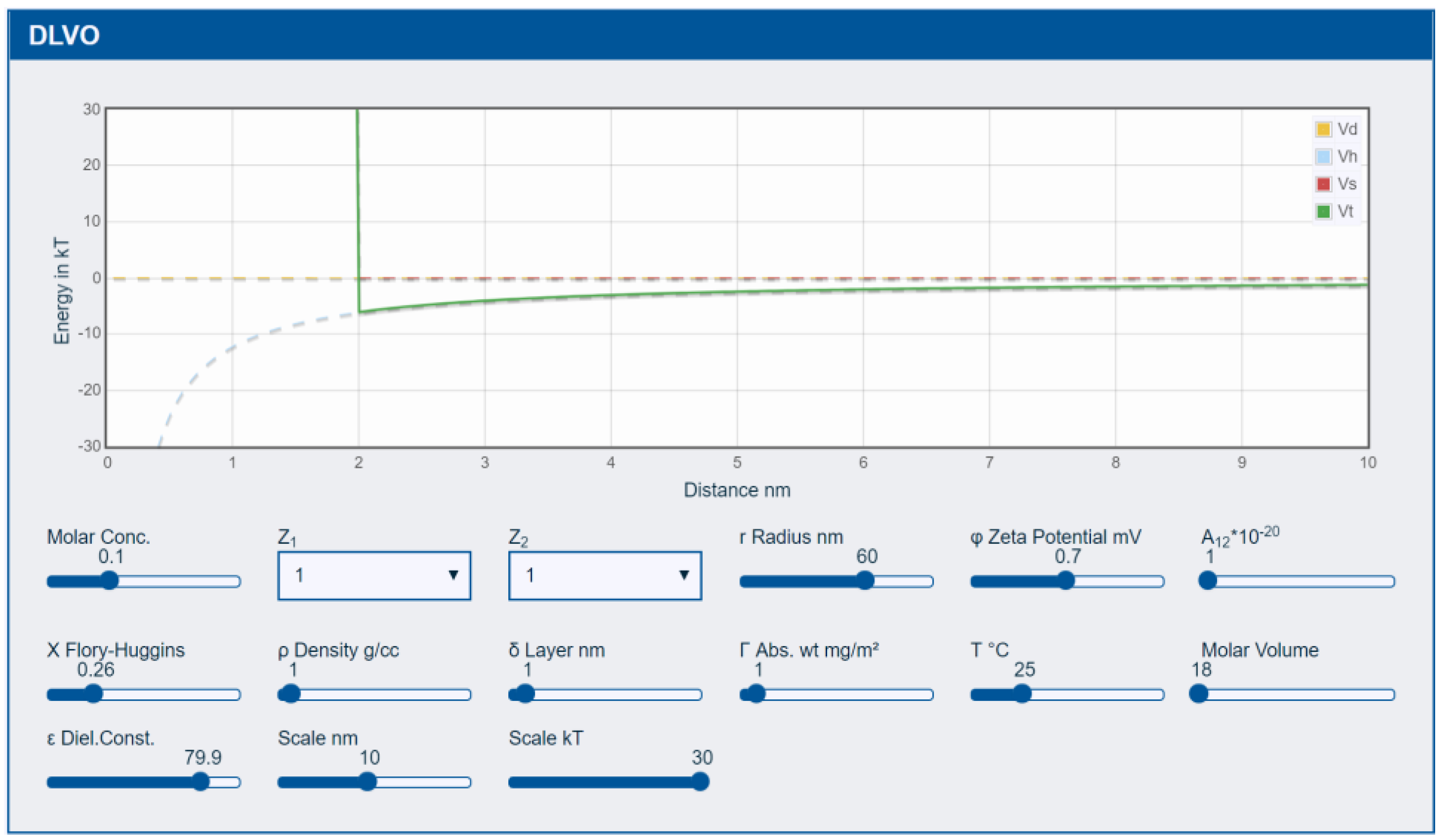
3.1. DLVO
3.2. Coating Defects
3.2.1. Pinholes
3.2.2. Levelling
3.2.3. Drop Spreading
3.2.4. Marangoni Defects
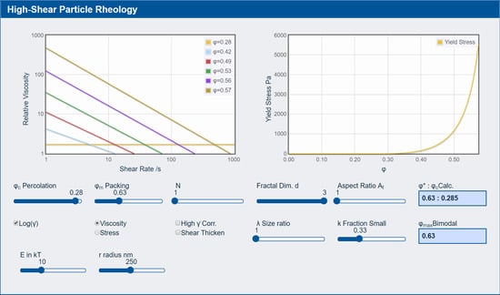
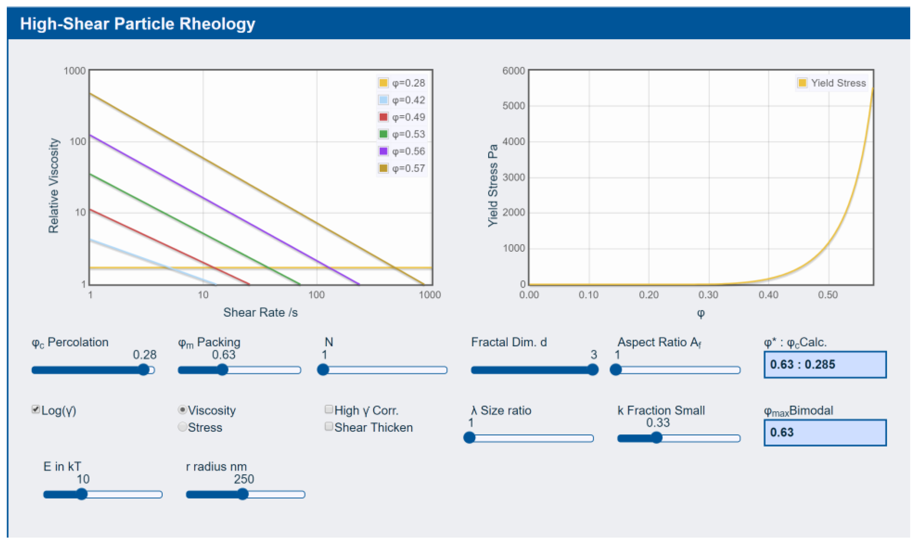
3.3. Rheology
3.4. Particles
Particle Solubility
4. Conclusions
Funding
Acknowledgments
Conflicts of Interest
References
- Derjaguin, B.; Landau, L.D. Acta Physicochim. USSR 1941, 14, 633. [Google Scholar]
- Verwey, E.W.; Overbeek, J.T.G. Theory of Stability of Lyophobic Colloids; Elsevier: Amsterdam, The Netherlands, 1948. [Google Scholar]
- Tadros, T. General Principles of Colloid Stability and the Role of Surface Forces. Colloid Stab. 2007, 1, 1–22. [Google Scholar]
- Steven, A. Printing Science: Principles and Practice. Available online: https://www.stevenabbott.co.uk/practical-coatings/the-book.php (accessed on 29 January 2019).
- Chalmers, I.; Glasziou, P. Avoidable waste in the production and reporting of research evidence. Lancet 2009, 374, 86–89. [Google Scholar] [CrossRef]
- Ioannidis, J.P.A. Why Most Published Research Findings Are False. PLoS Med. 2005, 2, e124. [Google Scholar] [CrossRef] [PubMed]
- A Platform for Open Science. Available online: https://www.materialscloud.org/home (accessed on 29 January 2019).
- Discover & Run Scientific Code. Available online: https://codeocean.com. (accessed on 29 January 2019).
- Hansen, C.M. Hansen Solubility Parameters, a User’s Handbook, 2nd ed.; CRC Press: Boca Raton, FL, USA, 2007. [Google Scholar]
- Asakura, S.; Oosawa, F. Interaction between particles suspended in solutions of macromolecule. J. Polym. Sci. 1958, 33, 183–192. [Google Scholar] [CrossRef]
- Sharma, A.; Ruckenstein, E. Energetic criteria for the breakup of liquid films on nonwetting solid surfaces. J. Colloid Interface Sci. 1990, 137, 433–445. [Google Scholar] [CrossRef]
- Edwards, A.M.; Ledesma-Aguilar, R.; Newton, M.I.; Brown, C.V.; McHale, G. Not spreading in reverse: The dewetting of a liquid film into a single drop. Sci. Adv. 2016, 2, e1600183. [Google Scholar] [CrossRef] [PubMed]
- Orchard, S.E. On surface levelling in viscous liquids and gels. App. Sci. Res. A 1963, 11, 451–464. [Google Scholar] [CrossRef]
- Tanner, L.H. The spreading of silicone oil drops on horizontal surfaces. J. Phys. D Appl. Phys. 1979, 12, 1473–1484. [Google Scholar] [CrossRef]
- McHale, G.; Newton, M.I.; Rowan, S.M.; Banerjee, M. The spreading of small viscous stripes of oil. J. Phys. D Appl. Phys. 1995, 28, 1925–1929. [Google Scholar] [CrossRef]
- Available online: https://www.stevenabbott.co.uk/practical-adhesion/ (accessed on 29 January 2019).
- Pearson, J.R.A. On convection cells induced by surface tension. J. Fluid Mech. 1958, 4, 489–500. [Google Scholar] [CrossRef]
- Dinkgreve, M.; Paredes, J.; Denn, M.M.; Bonn, D. On different ways of measuring “the” yield stress. J. Non-Newton. Fluid Mech. 2016, 238, 233–241. [Google Scholar] [CrossRef]
- Ferry, J.D. Viscoelastic Properties of Polymers, 3rd ed.; John Wiley & Sons: Hoboken, NJ, USA, 1980. [Google Scholar]
- Tschoegl, N.W. The Phenomenological Theory of Linear Viscoelastic Behavior; Springer: New York, NY, USA, 1989. [Google Scholar]
- Park, S.W.; Schapery, R.A. Methods of interconversion between linear viscoelastic material functions: Part I-a numerical method based on Prony series. Int. J. Solids Struct. 1999, 36, 1653–1675. [Google Scholar] [CrossRef]
- Petrie, C.J.S. Extensional viscosity: A critical discussion. J. Non-Newton. Fluid Mech. 2006, 137, 15–23. [Google Scholar] [CrossRef]
- Mewis, J.; Wagner, N.J. Colloidal Suspension Rheology; Cambridge University Press: Cambridge, UK, 2012. [Google Scholar]
- Krieger, I.M.; Dougherty, T.J. A mechanism for non-Newtonian flow in suspensions of rigid spheres. J. Rheol. 1959, 3, 137–152. [Google Scholar] [CrossRef]
- Yaron, I.; Gal-Or, B. On viscous flow and effective viscosity of concentrated suspensions and emulsions. Rheol. Acta 1972, 11, 241–252. [Google Scholar] [CrossRef]
- Pal, R. Novel viscosity equations for emulsions of two immiscible liquids. J. Rheol. 2001, 4, 509–520. [Google Scholar] [CrossRef]
- Campbell, G.A.; Zak, M.E.; Wetzel, M.D. Newtonian, power law, and infinite shear flow characteristics of concentrated slurries using percolation theory concepts. Rheol Acta 2018, 57, 197–216. [Google Scholar] [CrossRef]
- Bicerano, J.; Douglas, J.F.; Brune, D.A. Model for the Viscosity of Particle Dispersions. J. Macromol. Sci. 1999, 39, 561–642. [Google Scholar] [CrossRef]
- Flatt, R.J.; Bowen, P. Yodel: A Yield Stress Model for Suspensions. J. Am. Ceram. Soc. 2006, 89, 1244–1256. [Google Scholar] [CrossRef]
- Steven, A. Solubility Science: Principles and Practice. Available online: https://www.stevenabbott.co.uk/practical-solubility/the-book.php (accessed on 29 January 2019).
- Süß, S.; Sobisch, T.; Peukert, W.; Lerche, D.; Segets, D. Determination of Hansen parameters for particles: A standardized routine based on analytical centrifugation. Adv. Powder Technol. 2018, 29, 1550–1561. [Google Scholar] [CrossRef]
- Available online: https://www.hansen-solubility.com/HSP-science/sphere.php (accessed on 29 January 2019).
- Jones, A.; Vincent, B. Depletion Flocculation in Dispersions of Sterically-Stabilised Particles 2. Modifications to Theory and Further Studies. Colloid Surface 1989, 42, 113–138. [Google Scholar] [CrossRef]
- Available online: https://www.stevenabbott.co.uk/practical-solubility/kb.php (accessed on 29 January 2019).
- Available online: https://www.stevenabbott.co.uk/VR/ (accessed on 29 January 2019).


© 2019 by the author. Licensee MDPI, Basel, Switzerland. This article is an open access article distributed under the terms and conditions of the Creative Commons Attribution (CC BY) license (http://creativecommons.org/licenses/by/4.0/).
Share and Cite
Abbott, S. Practical Formulation Science for Particle-Based Inks. Colloids Interfaces 2019, 3, 23. https://doi.org/10.3390/colloids3010023
Abbott S. Practical Formulation Science for Particle-Based Inks. Colloids and Interfaces. 2019; 3(1):23. https://doi.org/10.3390/colloids3010023
Chicago/Turabian StyleAbbott, Steven. 2019. "Practical Formulation Science for Particle-Based Inks" Colloids and Interfaces 3, no. 1: 23. https://doi.org/10.3390/colloids3010023
APA StyleAbbott, S. (2019). Practical Formulation Science for Particle-Based Inks. Colloids and Interfaces, 3(1), 23. https://doi.org/10.3390/colloids3010023