Geometry-Aware 1D Residual CNN-BiLSTM Network for Automated Vertebral Localization and Scoliosis Classification

Abstract

Accurate localization of the upper end vertebra (UEV), lower end vertebra (LEV), and apex vertebra (AV) is essential for automated scoliosis assessment and Cobb angle measurement. This study proposes a geometry-aware, multi-task sequence learning framework for vertebral landmark localization and scoliosis type classification. The framework integrates YOLOv8-OBB-based feature extraction with a 1D Residual CNN-BiLSTM architecture and a displacement-guided regularization term, termed Geometric Loss (GeoLoss). Images and reference annotations were obtained from the open-source Spinal-AI2024 dataset, and a development set of 550 radiographs was used for model development and internal evaluation. Vertebral detections were transformed into 12-dimensional geometric sequences encoding orientation, displacement, shape, confidence, and curvature. Robustness was assessed using four train–validation–test partitioning strategies with repeated experiments and five-fold cross-validation, with the 75/15/10 partition showing the strongest mean internal performance. On a disjoint held-out set of 58 unseen images from the same dataset, the model achieved a Type Accuracy, EV Accuracy (±1), and EV Accuracy (±2) of 96.55%, 86.63%, and 94.19%, respectively, with an EV mean absolute error of 0.559 vertebral levels. These findings support geometry-aware sequence modeling as an effective approach for automated vertebral landmark localization and scoliosis assessment.

1. Introduction

Adolescent idiopathic scoliosis (AIS) is one of the most common spinal deformities encountered in clinical practice [1,2]. Clinical assessment of scoliosis severity relies primarily on Cobb angle measurement, which is determined by the relative orientation of the upper end vertebra (UEV) and lower end vertebra (LEV) on coronal spinal radiographs [3,4]. Curve magnitude and configuration are also important factors in selecting conservative treatment strategies and guiding follow-up [5]. The apex vertebra (AV), located near the point of maximum lateral deviation of the spinal curve, provides additional information on curve location and morphology [6]. However, manual identification of these vertebral landmarks is time-consuming and subject to inter-observer variability, potentially affecting measurement reproducibility [7].

To improve measurement reproducibility and clinical efficiency, numerous computer-aided diagnosis (CAD) systems have been developed for automated scoliosis assessment [8,9]. Recent advances in deep learning have enabled automated vertebral detection, spinal centerline estimation, landmark localization, and Cobb angle measurement using convolutional neural networks (CNNs) and advanced object detection architectures [4,10]. Among these approaches, region-based and single-shot detectors like the YOLO (You Only Look Once) architecture have demonstrated strong potential for vertebral localization due to their high computational efficiency and robust spatial localization performance [11,12].

Despite these advances, automated end-vertebra selection remains a challenging task [9,10]. Most existing approaches focus primarily on coarse vertebral detection or segmentation; consequently, clinically crucial landmarks such as the UEV, LEV, and AV are frequently derived using handcrafted rule-based or post-processing procedures [8,10]. Furthermore, current methods often treat vertebrae as independent entities, failing to exploit the sequential anatomical dependencies inherent to the human spine [13,14]. Because they overlook these spatial constraints, standard landmark localization performance deteriorates when vertebral orientation, displacement, and morphology change progressively across adjacent vertebral levels [13,15].

To address these limitations, this study proposes a geometry-aware, multi-task sequence learning framework for automated vertebral landmark localization and scoliosis type classification. Unlike conventional approaches that treat individual vertebrae independently or identify clinically relevant landmarks using handcrafted post-processing heuristics, our framework explicitly models the vertebral column as an ordered anatomical sequence.

In this pipeline, YOLOv8-OBB detections are first transformed into structured 12-dimensional geometric descriptors that encode vertebral orientation, lateral displacement, shape, detection confidence, and spinal curvature characteristics. Furthermore, a displacement-guided geometric regularization strategy, termed Geometric Loss (GeoLoss), is integrated into the multi-task optimization process to ensure anatomically consistent landmark predictions [16,17].

This study makes three main contributions. First, vertebral detections are represented as a 12-dimensional geometric sequence that integrates orientation, displacement, shape, confidence, and curvature-related information. Second, a multi-task 1D Residual CNN-BiLSTM framework is developed to jointly perform scoliosis type classification and vertebral landmark localization while exploiting the ordered structure of the spine. Third, GeoLoss incorporates displacement-based geometric information into the optimization process to improve the consistency of vertebral landmark predictions.

The proposed framework is further evaluated using repeated data partitions, five-fold cross-validation, and a disjoint held-out test set from the same source dataset. These complementary evaluation strategies provide a more comprehensive assessment of the model’s robustness and generalization performance.

The remainder of this paper is organized as follows. Section 2 reviews related work on automated scoliosis assessment and compares representative deep learning approaches. Section 3 details the dataset and annotation process, vertebral feature extraction, the proposed 1D Residual CNN-BiLSTM architecture, the multi-task prediction strategy, GeoLoss, and the experimental protocol. Section 4 presents and discusses the experimental results, including repeated data-partition experiments, five-fold cross-validation, ablation studies, and evaluation on a disjoint held-out test set. Finally, Section 5 summarizes the main findings and concludes the paper.

2. Literature Overview

Deep learning methods have been applied to various stages of automated scoliosis assessment. Horng et al. [3] segmented individual vertebrae using U-Net variants and subsequently estimated spinal curvature based on the Cobb angle criterion. In contrast, Dubost et al. [8] extracted the spinal centerline using cascaded convolutional neural networks and estimated Cobb angles from the resulting smoothed centerline. Chen et al. [9] formulated Cobb angle estimation as a regression problem, employing separate networks for landmark and angle prediction. Rather than directly estimating the Cobb angle, Wang et al. [10] localized vertebral corner landmarks using a multi-stage cascaded CNN with a shape constraint. Collectively, these segmentation-, centerline-, regression-, and landmark-based approaches provide distinct pathways for automated scoliosis assessment; however, their underlying representations and prediction targets differ substantially.

To capture finer clinical details, attention-enhanced convolutional architectures have improved scoliosis-related image analysis by selectively emphasizing relevant anatomical regions [18]. Similarly, attention-based segmentation networks have demonstrated diagnostic performance comparable to that of experienced clinicians in automated screening tasks [18]. YOLO-based object detection provides another approach to vertebral localization. Liu et al. [11] used a YOLOv8n-OBB-based detector to identify oriented vertebral objects and subsequently estimate Cobb angles from the detections, whereas Laazab et al. [12] combined YOLOv8-based vertebral localization with U-Net segmentation in spinal MRI. Although both approaches employ object detection to identify vertebral structures, their downstream objectives differ: the former derives Cobb-angle measurements from orientation-aware detections, whereas the latter uses localization as a precursor to vertebral segmentation.

In the present study, YOLOv8-OBB similarly serves as a front-end localization module; however, its outputs are further transformed into geometric descriptors for subsequent vertebral sequence modeling rather than being used as the final analytical output. This distinction enables the detected vertebral structures to be represented as an ordered geometric sequence for downstream multi-task prediction.

Despite these advances, most existing frameworks still treat end-vertebra selection as a detached post-processing step following vertebral detection or landmark regression [9]. Such approaches often rely on handcrafted geometric rules and fail to fully exploit the ordered anatomical relationships inherent among vertebrae. Furthermore, maintaining anatomical consistency across neighboring vertebrae remains challenging because vertebral morphology changes gradually along the spinal column [15].

To address these limitations, several recent studies have incorporated anatomical constraints, shape priors, or consistency-based learning mechanisms into vertebral localization and segmentation frameworks [16,19]. Anatomy-guided representation learning likewise aims to preserve structural information during medical image analysis [19,20]. Meng et al. [13] combined deep-network predictions with graph optimization and statistical priors to enforce anatomically consistent vertebral localization, segmentation, and identification in CT images, whereas Alsharif et al. [15] represented vertebrae and intervertebral discs as graph nodes linked by anatomical relationships for MRI segmentation. Although these approaches share the goal of incorporating anatomical information, they differ in how such information is encoded, ranging from statistical priors to explicit graph-based relationships.

Because the vertebral column forms a naturally ordered anatomical structure, sequential learning approaches offer a promising strategy for modeling inter-vertebral dependencies [21]. For instance, Transformer-based deep learning models have been introduced for automated spine image interpretation, demonstrating the strong capability of attention mechanisms in capturing clinically relevant spinal features [22]. More broadly, previous deep learning studies emphasize that spinal analysis benefits significantly from explicitly modeling these structural and positional relationships [15,23]. This holistic perspective is especially critical in conditions like scoliosis, where disease progression is tightly linked to global radiographic characteristics of the spinal deformity rather than isolated vertebral observations [24].

To capture these ordered patterns, researchers have frequently employed specialized recurrent and convolutional architectures. Specifically, Long Short-Term Memory (LSTM) networks are well suited to capturing contextual dependencies in sequential biomedical data [21], whereas one-dimensional convolutional neural networks (1D-CNNs) effectively extract local structural patterns from ordered feature sequences [25]. Combining these complementary strengths, hybrid CNN-BiLSTM architectures integrate local feature extraction with long-range sequence modeling [26].

Table 1. Comparison of representative approaches for automated spinal and vertebral analysis.

Study	Imaging/Primary Task	Core Approach	Structural/Geometric Modeling	Main Output
Horng et al. [3]	X-ray/Cobb angle measurement	U-Net, Dense U-Net, and Residual U-Net	Vertebral morphology derived from segmentation	Vertebral segmentation and Cobb angles
Dubost et al. [8]	X-ray/spinal curvature estimation	Cascaded CNNs	Smoothed spinal centerline	Cobb angles
Chen et al. [9]	X-ray/Cobb angle estimation	AEC-Net regression framework	Landmark and angle information modeled using separate networks	Cobb angles
Wang et al. [10]	X-ray/vertebral landmark localization	Multi-stage cascaded CNN	PCA-based vertebral shape constraint	Vertebral corner landmarks
Liu et al. [11]	X-ray/vertebral detection and Cobb angle measurement	YOLOv8-DSF based on YOLOv8n-OBB	Vertebral orientation and OBB geometry	Rotational vertebral detections and Cobb angles
Meng et al. [13]	CT/localization, segmentation, and identification	Deep networks with graph optimization	Anatomical consistency through statistical priors and graphical modeling	Vertebral localization, segmentation, and labels
Aydogdu et al. [14]	CT/segmentation and centroid localization	Multi-task network with Vision Transformer bottleneck	Global spatial context	Vertebral masks and centroids
Alsharif et al. [15]	MRI/vertebra and intervertebral-disc segmentation	Graph convolutional segmentation framework	Explicit graph-based anatomical relationships	Vertebral and intervertebral-disc segmentation
Proposed framework	X-ray/scoliosis classification and vertebral landmark localization	YOLOv8-OBB + 1D Residual CNN-BiLSTM + GeoLoss	Ordered 12-dimensional geometric sequence with displacement-guided regularization	C/S type and UEV, LEV, and AV levels

summarizes representative approaches that illustrate these methodological differences. Because the studies employ different imaging modalities, datasets, target tasks, and evaluation metrics, the table emphasizes methodological characteristics rather than direct numerical comparisons of performance.

Motivated by these observations, this study formulates scoliosis landmark localization as a geometry-aware sequence learning problem. Unlike existing approaches that primarily rely on independent vertebral detection, segmentation, or handcrafted post-processing rules [10], the proposed framework first extracts orientation-aware vertebral descriptors from YOLOv8-OBB detections [11] and subsequently models the resulting sequence using a 1D Residual CNN-BiLSTM multi-task architecture. Furthermore, a displacement-guided geometric regularization strategy (GeoLoss) is introduced to incorporate anatomical priors during optimization. This enhances landmark localization consistency while remaining fully compatible with end-to-end gradient-based optimization.

3. Materials and Methods

3.1. Dataset and Annotation

The data used in this study were obtained from the open-source Spinal-AI2024 dataset, released alongside the CurvNet framework [27]. This resource contains 20,000 synthetic scoliosis radiographs paired with vertebral and Cobb-related annotations. These source images and annotations were utilized directly, with the provided annotations serving as the reference ground truth for subsequent model development and evaluation.

From the original dataset, 550 images were manually screened and selected for model development and internal evaluation. Images were included if the vertebral structures and their corresponding annotations were sufficiently clear and complete for reliable landmark identification. Conversely, images demonstrating incomplete vertebral coverage, obscured anatomical structures, or ambiguous annotations were excluded. This screening process served solely to select suitable samples; the original image content and dataset-provided annotations remained unmodified.

An additional 58 images satisfying the same quality and completeness criteria were reserved from the Spinal-AI2024 dataset to serve as a disjoint, held-out test set. To ensure evaluation integrity, these images were entirely excluded from the 550-image development cohort and remained completely unseen during training, hyperparameter tuning, and checkpoint selection. Ultimately, this final test partition comprised 30 C-type and 28 S-type cases.

For each annotated spinal curve, the UEV and LEV were determined using the dataset’s Cobb-angle annotations. Specifically, the vertebrae corresponding to the superior and inferior boundaries of the Cobb measurement were recorded as the UEV and LEV, respectively. Together, these two landmarks define the precise vertebral levels used for Cobb angle assessment [3,4].

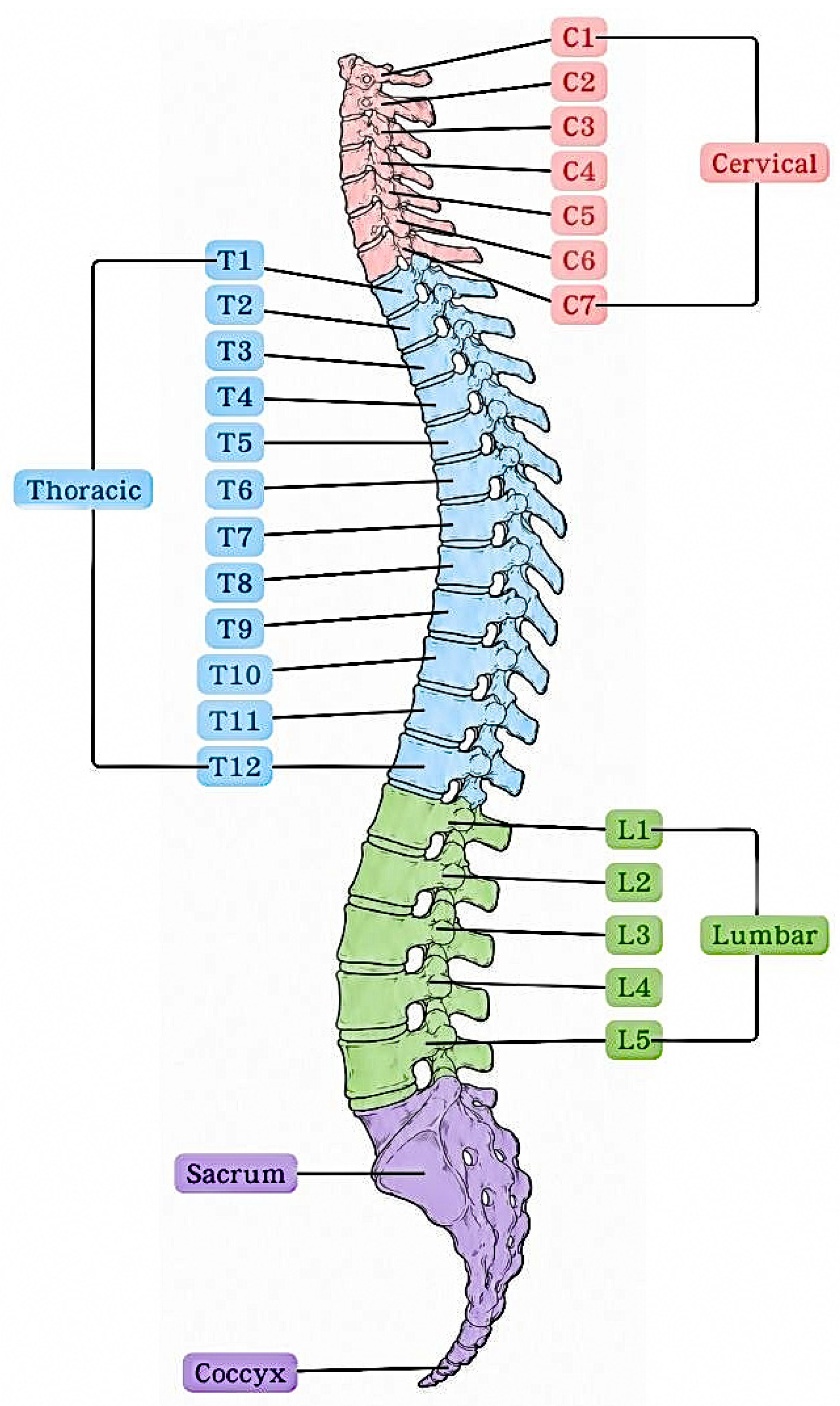
To facilitate interpretation of the vertebral labels used throughout the manuscript, Figure 1 illustrates the major spinal regions and corresponding vertebral numbering. The vertebral region analyzed in this study spans T1–L5.

The AV label was determined independently based on vertebral geometry. For each annotated curve, the AV was assigned to the vertebra exhibiting the maximum lateral displacement relative to the estimated spinal centerline. Consequently, while the UEV and LEV labels were derived directly from the original Cobb-related annotations, the AV label was algorithmically generated using this lateral-displacement criterion. This definition aligns with the standard clinical interpretation of the apex as the vertebra located nearest to the maximum lateral deviation of the spinal curve [6].

Because the AV labels were algorithmically derived using this geometric rule, the displacement-guided GeoLoss (introduced in Section 3.5) was designed as an auxiliary consistency regularizer rather than an independent source of anatomical supervision. Its primary purpose was to encourage AV predictions to remain mathematically consistent with the predefined geometric landmark criterion during training.

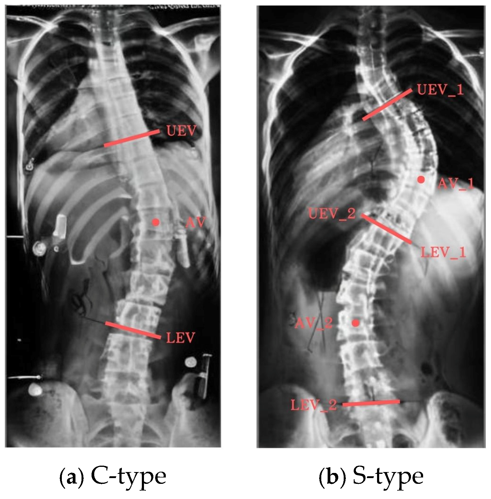
Scoliosis commonly presents as either a dominant single-curve configuration or a multiple-curve pattern with compensatory components [1,2,24]. Based on this clinical framework and the annotated curvature configurations, each image in this study was categorized as either C-type or S-type scoliosis. C-type cases featured a single dominant curve and were represented by one set of UEV, LEV, and AV labels. In contrast, S-type cases contained two distinct curves, with separate sets of UEV, LEV, and AV labels assigned to each curve component. Representative C-type and S-type radiographs, along with their corresponding vertebral landmarks, are shown in Figure 2.

The 550 selected images constituted the core model-development dataset, which was utilized for training, validation, internal testing, repeated partition experiments, and five-fold cross-validation.

To ensure rigorous performance assessment, a separate, disjoint held-out set of 58 previously unseen images was selected from the same Spinal-AI2024 source dataset for final evaluation [27]. Crucially, none of these 58 images were involved in model training, validation, internal testing, hyperparameter optimization, or checkpoint selection. This held-out cohort comprised 30 C-type and 28 S-type cases. Because each C-type image features a single curve and each S-type image features two, the held-out set provided a total of 86 unique spinal curves for evaluation.

Following annotation processing, vertebral detections were generated using YOLOv8-OBB and subsequently transformed into fixed-length geometric feature sequences for downstream sequence modeling. The data-partitioning strategy and evaluation metrics are described in Section 3.6. As this study involved only secondary computational analysis of publicly available images and existing annotations, no new clinical data were collected, no human participants were directly recruited, and no identifiable patient information was accessed. In addition, potential diurnal variation in Cobb-angle-related annotations was not separately evaluated [9].

3.2. Vertebral Feature Extraction

Prior to sequence modeling, vertebral geometric attributes were extracted utilizing a YOLOv8-OBB detector. Unlike conventional axis-aligned horizontal bounding boxes, the YOLOv8-OBB architecture provides orientation-aware object detections, which yield precise vertebral center coordinates, bounding-box dimensions, rotation angles, and detection confidence scores [11]. These parameters effectively preserve critical vertebral orientation information, providing a compact yet highly expressive representation of spinal morphology for automated scoliosis assessment.

In this study, a YOLOv8n-OBB model was employed as the orientation-aware vertebral detector. The network comprises a feature-extraction backbone, a multi-scale feature-fusion neck, and an oriented detection head. The backbone extracts hierarchical image features, while the neck integrates information across multiple feature scales. The oriented detection head predicts the center coordinates, width, height, rotation angle, and confidence score for each detected vertebra. Accordingly, each oriented bounding box (OBB) can be represented as ($c_x$, $c_y$, w, h, θ), where $c_x$ and $c_y$ denote the bounding-box center coordinates, w and h denote its width and height, respectively, and θ denotes the vertebral orientation.

A separate YOLO-based detector was employed to identify the vertebral levels from T1 to T12 and L1 to L5. The detected vertebral levels were matched to the corresponding OBB detections based on spatial proximity. This matching associated the orientation and geometric information obtained from YOLOv8n-OBB with the anatomical vertebral labels required for subsequent sequence construction.

Following vertebral detection, all vertebral bodies were sorted sequentially according to their anatomical positions from the upper thoracic region to the lower lumbar region, thereby establishing an ordered vertebral sequence. This representation transforms the continuous spinal column into a structured anatomical sequence in which neighboring vertebrae maintain meaningful spatial relationships [15,23]. Previous studies have shown that incorporating such structural and positional relationships can significantly improve representation learning for spinal image analysis [23].

To quantitatively characterize vertebral geometry and spinal curvature, a 12-dimensional geometric descriptor was constructed for each detected vertebra. These features capture comprehensive information regarding vertebral orientation, lateral displacement, geometric shape, detection confidence, and spatial inter-vertebral relationships. The complete definitions of these geometric features are systematically summarized in

Table 2. Detailed Definitions of the 12-Dimensional Geometric Feature Set.

Feature Index	Feature Name	Description
F1	Vertebral Angle	Orientation angle of the vertebral body obtained from YOLOv8-OBB detection
F2	Lateral Distance	Horizontal displacement relative to the estimated spinal centerline
F3	Relative Distance	Lateral displacement referenced to the first vertebra in the sequence
F4	Normalized Distance	Lateral displacement normalized by the global displacement range
F5	Distance Sign	Sign of lateral displacement
F6	Side Indicator	Encodes left/right deviation direction
F7	Width Height Ratio	Bounding-box width divided by height
F8	Detection Confidence	Confidence score produced by YOLOv8-OBB
F9	Angle Difference	Orientation difference relative to the previous vertebra
F10	Distance Difference	Displacement difference relative to the previous vertebra
F11	Curve Range	Global displacement range across the vertebral sequence
F12	Curve Energy	Mean absolute displacement across the vertebral sequence

.

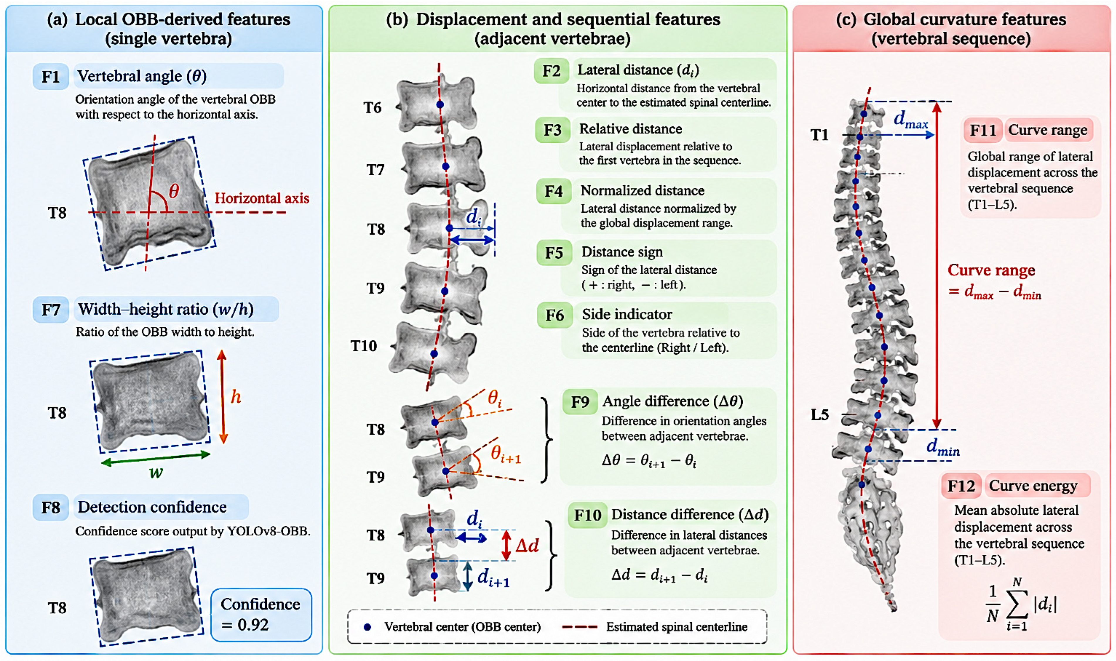
To complement the definitions in Table 2, Figure 3 illustrates how the 12 geometric features are derived from individual vertebral detections and the resulting ordered vertebral sequence.

The proposed feature representation is grouped into five complementary categories. Orientation-related features (F1 and F9) characterize vertebral tilt and local angular transitions. Displacement features (F2–F6 and F10) capture lateral deviation patterns and spatial relationships relative to the spinal centerline, providing critical insights for the biomechanical characterization of scoliosis [2,6].

Shape-related properties are captured by the width-height ratio (F7), while detection confidence (F8) provides a direct estimate of measurement reliability. Finally, global curvature characteristics are captured via curve range and curve energy descriptors (F11 and F12), which summarize the overall displacement distribution across the entire spinal sequence.

Together, these descriptors transform raw vertebral detections into a compact geometric sequence representation that is invariant to image scale and well-suited for sequential learning. Similar structure-aware learning strategies have been shown to enhance the extraction of anatomically meaningful features in various spinal imaging applications [23].

Because the number of detected vertebrae varies across patients, all vertebral sequences were padded to a fixed maximum length prior to network training. This standardization accommodates mini-batch processing while preserving the original anatomical ordering and structural integrity of the vertebral column.

3.3. Proposed Model Architecture

The proposed framework utilizes a hybrid 1D Residual CNN-BiLSTM architecture to simultaneously execute scoliosis classification and vertebral landmark localization from geometric sequences. The network ingests an ordered sequence of 12-dimensional vertebral descriptors, processing them through a shared feature extraction backbone.

First, local geometric patterns are extracted using a one-dimensional residual convolutional neural network (1D Residual CNN). One-dimensional convolutions are well suited for extracting local structural patterns from ordered feature sequences [25]. This CNN-based feature extraction allows convolutional layers to automatically learn discriminative local representations [28]. Furthermore, compact CNN architectures balance robust feature extraction, computational complexity, and model interpretability in medical-imaging applications [29].

In our framework, the convolutional filters operate along the ordered vertebral sequence rather than directly on radiographic pixels. This design captures localized variations in vertebral orientation, lateral displacement, and shape characteristics. Consequently, this stage produces compact geometric representations of scoliosis-related spinal deformation, which serve as inputs for subsequent bidirectional sequence modeling.

The resulting feature maps are subsequently processed by a BiLSTM network. LSTM networks are designed to capture long-range dependencies in sequential data. By processing sequences in both forward and backward directions, BiLSTM networks further enhance the modeling of sequential dependencies and contextual information [21,26].

Unlike unidirectional models, the BiLSTM architecture analyzes the vertebral sequence simultaneously in both cranial-to-caudal and caudal-to-cranial directions. This bidirectional processing enables the framework to capture holistic contextual relationships across the entire spinal column, thereby better exploiting the ordered anatomical structure of vertebral sequences.

The combination of 1D Residual CNN-based local feature extraction and BiLSTM-based contextual modeling has proven highly effective in various biomedical analysis tasks that require concurrent local feature representation and long-range dependency modeling [26]. Inspired by these successes, the proposed framework integrates a 1D Residual CNN and BiLSTM modules to simultaneously capture local vertebral morphology and global anatomical dependencies.

Such complementary representations are particularly beneficial for vertebral landmark localization. In this task, clinically relevant landmarks are inherently influenced not only by local geometric characteristics but also by their relative positions within the macro-structural spinal architecture [15,23].

The feature representations generated by the BiLSTM layer are shared across multiple prediction branches within a multi-task learning framework [14,30]. By jointly learning scoliosis classification and vertebral landmark localization, the network leverages complementary anatomical insights while maintaining a unified sequence representation. This design facilitates cross-task knowledge transfer, thereby improving overall learning efficiency and model generalization.

3.4. Parallel Multi-Task Softmax Classifiers

The shared feature representation generated by the CNN-BiLSTM backbone is simultaneously optimized for scoliosis classification and vertebral landmark localization through a parallel multi-task learning strategy [30]. Similar multi-task frameworks have been successfully applied to vertebral analysis tasks, where shared representations are leveraged to optimize multiple anatomically related objectives.

Furthermore, the literature indicates that the joint optimization of classification and localization tasks improves feature-sharing efficiency. This simultaneous learning paradigm enhances model generalization and facilitates the extraction of complementary information across related tasks [28].

The framework incorporates a multi-branch architecture: an image-level classification branch for scoliosis curve-type prediction, alongside distinct curve-level landmark branches for UEV, LEV, and AV localization. For C-type images, the network evaluates a single set of curve-specific landmarks. In contrast, for S-type images, it evaluates two separate landmark sets corresponding to the distinct curve components. All prediction branches share the feature representations generated by the joint 1D Residual CNN-BiLSTM backbone while simultaneously producing task-specific probability distributions.

For each prediction task, the shared feature representation is projected through a fully connected layer followed by a Softmax activation function to yield a probability distribution over all candidate classes:

$$p_i={\displaystyle \frac{\exp (z_i)}{{\displaystyle \sum _{j=1}^K\exp }(z_j)}},$$

(1)

where $z_i$ denotes the logit of class $i$, K represents the number of candidate classes, and $p_i$ is the predicted probability.

The final prediction is obtained by selecting the class with the highest probability:

$$\widehat{y}=\arg {\max }_i{p}_i,$$

(2)

For image-level classification, the network predicts either C-type or S-type scoliosis. For curve-level landmark localization, each valid curve component generates distinct probability distributions across candidate vertebral levels to predict the UEV, LEV, and AV.

The classification objective for each prediction branch is formulated using categorical cross-entropy loss:

$$L_{CE}=-{\displaystyle \sum _{i=1}^K{y}_i}\log (P_i),$$

(3)

where $y_i$ denotes the ground-truth label and $P_i$ represents the predicted probability.

The total multi-task classification loss is computed as the sum of the individual branch losses:

$$L_{MT}= L_{Type}+L_{UEV}+L_{LEV}+L_{AV},$$

(4)

The geometry-aware regularization term introduced in the following section is combined with the multi-task classification objective to form the final optimization function.

3.5. Geometry-Aware Optimization with GeoLoss

Although the multi-task classification framework effectively learns vertebral landmark localization via categorical supervision, the resulting probability distributions can become spatially dispersed across neighboring vertebrae. This dispersion is particularly pronounced when geometric variations between adjacent vertebrae are subtle—a phenomenon that can degrade localization precision and yield anatomically inconsistent predictions [13].

To address this limitation, we introduce a geometry-aware regularization term, called GeoLoss, which incorporates anatomical displacement information directly into the optimization process [17]. The integration of such anatomical priors into deep learning optimization has been shown to improve anatomical consistency and localization accuracy in medical image analysis [20].

This framework assumes that vertebrae with greater lateral displacements relative to the spinal centerline are more likely to represent clinically significant anatomical landmarks. This premise is grounded in the anatomical observation that the apex vertebra is located near the maximum lateral deviation of the spinal curve [6].

Furthermore, previous studies have demonstrated that incorporating explicit geometric constraints can improve anatomical consistency and structural plausibility during medical image analysis [17]. Therefore, the predicted probability distribution should concentrate around these geometrically prominent vertebrae rather than being uniformly distributed across neighboring candidates.

Let $d_i$ denote the normalized lateral displacement of the $i$ vertebra and $p_i$ denote the probability assigned by the landmark classification branch. The expected displacement derived from this predicted probability distribution is defined as:

$$D_{exp}={\displaystyle \sum _{i=1}^N{p}_i}{d}_i,$$

(5)

where N denotes the number of vertebrae in the sequence. The maximum observed displacement within this sequence is defined as follows:

$$D_{max}={\max }_i(d_i),$$

(6)

and GeoLoss is then formulated as follows:

$$L_{Geo}=\left|D_{max}-D_{\exp }\right|.$$

(7)

For a mini-batch containing B samples, the batch-level GeoLoss is computed as follows:

$$L_{Geo}^{Batch}={\displaystyle \frac{1}{B}}{\displaystyle \sum _{b=1}^B{L}_{Geo}^{(b)}}.$$

(8)

The final optimization objective combines the multi-task classification loss with the proposed geometric regularization term:

$$L_{Total}=L_{MT}+\lambda L_{GEO},$$

(9)

where λ controls the contribution of the geometric regularization term.

By minimizing the discrepancy between the expected displacement and the maximum observed displacement, GeoLoss encourages the network to allocate greater probability mass to geometrically salient vertebrae, thereby enhancing geometric consistency during optimization [17]. This mechanism provides a robust anatomical prior that improves landmark localization consistency while fully preserving the end-to-end differentiability of the training process [17,19].

3.6. Experimental Protocol and Evaluation Metrics

The 550-image development set was evaluated using four train–validation–test partitioning strategies: 80/10/10, 75/15/10, 70/15/15, and 60/20/20. For each strategy, the dataset was independently randomized, and the complete training and evaluation pipeline was repeated five times. Within each partition, the training subset was utilized for model parameter optimization, the validation subset for checkpoint selection, and the internal test subset exclusively for final evaluation following model selection.

To quantify model sensitivity to varying data compositions and ensure robust performance reporting [28], the results across all five runs were summarized using the mean and standard deviation. This repeated evaluation across randomized data splits minimizes dependency on any single data partition, thereby enhancing the reliability and reproducibility of the reported metrics [28,31].

To ensure robustness, we selected the default partitioning strategy based on the average performance across five independent runs rather than the peak result of a single randomized trial. The 75/15/10 configuration yielded the highest mean Type Accuracy, EV Accuracy (±1), and EV Accuracy (±2). Consequently, this setup was adopted for all subsequent ablation studies and model comparisons.

To evaluate performance stability and generalization across distinct data subsets [31], we performed five-fold cross-validation on the 550-image development set. For each fold, four subsets were used for model development while the remaining subset was reserved for testing, ensuring each image served as test data exactly once. We report the fold-specific results alongside their corresponding mean and standard deviation for both scoliosis type classification and vertebral landmark localization.

Following internal experimentation, we utilized a disjoint held-out test set from the Spinal-AI2024 source dataset for the final evaluation [27]. This benchmarking set contained 58 previously unseen images that were strictly excluded from model training, validation, internal testing, hyperparameter tuning, and checkpoint selection.

For this evaluation, we retained the fourth run of the 75/15/10 configuration as the final frozen model, as it yielded the highest Type Accuracy and EV Accuracy (±1) among the five experimental runs. Crucially, no model parameters or decision rules were modified after testing on this held-out set.

Scoliosis type classification was evaluated at the image level. To evaluate performance across different spinal curvatures, class-specific accuracies were computed independently for C-type and S-type scoliosis as follows:

$$AC{C}_c={\displaystyle \frac{N_{correct,c}}{N_c}}\times 100\%,$$

(10)

where $N_{correct,c}$ denotes the number of correctly classified images belonging to class $c$, and $N_c$ denotes the total number of images in that class. To reduce the influence of differences in class distribution, the primary Type Accuracy used in the repeated partition experiments was the macro-average of the C-type and S-type accuracies:

$$\mathrm{Type} \mathrm{Accuracy}={\displaystyle \frac{AC{C}_C+AC{C}_S}{2}}.$$

(11)

For the held-out test set, overall image-level accuracy was calculated as the ratio of correctly classified images to the total evaluated. Vertebral landmark localization was then assessed using the absolute difference between the predicted and reference vertebral levels, where levels from T1 to L5 were represented as ordered indices. For the i-th landmark, the localization error was defined as:

$$e_i=\left|{\widehat{v}}_i-v_i\right|,$$

(12)

where ${\widehat{v}}_i$ and $v_i$ denote the predicted and reference vertebral indices, respectively.

End-vertebra accuracy within a tolerance of k vertebral levels was defined as:

$$\mathrm{EV} \mathrm{Accuracy} (\pm k)={\displaystyle \frac{1}{N_{EV}}}{\displaystyle \sum _{i=1}^{N_{EV}}\mathbb{I}}\left(e_i\le k\right)\times 100\%,$$

(13)

where k ∈ {1, 2}, $N_{EV}$ represents the total number of expected UEV and LEV annotations, and $\mathbb{I}(\cdot )$ is the indicator function. Consequently, a prediction was considered correct under EV Accuracy (±1) if it fell on the reference vertebra or an immediately adjacent level, and under EV Accuracy (±2) if it fell within a two-level tolerance.

Because C-type and S-type cases contained one and two annotated curves, respectively, vertebral landmark localization was evaluated exclusively for anatomically valid curve components. Specifically, each C-type case contributed one set of UEV, LEV, and AV annotations, whereas each S-type case contributed two sets corresponding to its dual curves. Landmark predictions for nonexistent curve components were excluded from curve-level evaluation. Consequently, only valid ground-truth landmarks contributed to the denominators of the localization accuracy, mean absolute error, and detection-coverage metrics.

The mean absolute error of the successfully detected end vertebrae was defined as follows:

$$\mathrm{EV} \mathrm{MAE}={\displaystyle \frac{1}{N_{det}}}{\displaystyle \sum _{i=1}^{N_{det}}{e}_i},$$

(14)

where $N_{det}$ denotes the number of successfully detected end vertebrae. Detection coverage was defined as follows:

$$\mathrm{Detection} \mathrm{Coverage}={\displaystyle \frac{N_{det}}{N_{EV}}}\times 100\%$$

(15)

In addition to the aggregate end-vertebra metrics, localization accuracy (within ±1 and ±2 levels) and mean absolute error (MAE) were calculated separately for the UEV, LEV, and AV to evaluate landmark-specific performance.

4. Results and Discussion

4.1. Performance Under Different Data Partitioning Strategies

The proposed framework was evaluated using four distinct train–validation–test data splits: 80/10/10, 70/15/15, 75/15/10, and 60/20/20. This experiment aimed to investigate how different data allocation strategies affect both scoliosis type classification and vertebral landmark localization performance. To minimize bias from any single randomized split and quantify performance variability, each partitioning strategy was evaluated independently over five random trials.

For each experimental run, we calculated the macro-averaged Type Accuracy, class-specific accuracies for C-type and S-type scoliosis, and EV Accuracy within tolerances of one [EV Accuracy (±1)] and two [EV Accuracy (±2)] vertebral levels. The detailed results and corresponding summary statistics are presented in

Table 3. Model performance across different data partitioning ratios (Trial 1).

Partitioning Ratio	Type Accuracy (C/S)	EV Accuracy (±1)	EV Accuracy (±2)
80/10/10	84.59% (80.00%/89.19%)	83.04%	89.47%
70/15/15	79.25% (65.52%/92.98%)	78.10%	85.85%
75/15/10	86.78% (81.25%/92.31%)	80.75%	85.63%
60/20/20	81.71% (69.05%/94.37%)	78.47%	84.66%

,

Table 4. Model performance across different data partitioning ratios (Trial 2).

Partitioning Ratio	Type Accuracy (C/S)	EV Accuracy (±1)	EV Accuracy (±2)
80/10/10	86.89% (90.00%/83.78%)	80.12%	85.96%
70/15/15	71.70% (54.76%/88.64%)	73.84%	79.65%
75/15/10	92.98% (96.67%/89.29%)	86.21%	91.38%
60/20/20	83.15% (80.00%/86.30%)	80.53%	86.29%

,

Table 5. Model performance across different data partitioning ratios (Trial 3).

Partitioning Ratio	Type Accuracy (C/S)	EV Accuracy (±1)	EV Accuracy (±2)
80/10/10	80.29% (70.59%/90.00%)	81.29%	86.26%
70/15/15	74.54% (59.26%/89.83%)	81.01%	88.18%
75/15/10	81.66% (71.43%/91.89%)	83.05%	87.93%
60/20/20	90.72% (92.11%/89.33%)	82.15%	87.61%

,

Table 6. Model performance across different data partitioning ratios (Trial 4).

Partitioning Ratio	Type Accuracy (C/S)	EV Accuracy (±1)	EV Accuracy (±2)
80/10/10	89.47% (89.47%/89.47%)	81.29%	88.59%
70/15/15	85.12% (76.92%/93.33%)	82.75%	89.34%
75/15/10	97.22% (100.00%/94.44%)	88.51%	90.25%
60/20/20	84.47% (81.25%/87.69%)	79.06%	84.96%

,

Table 7. Model performance across different data partitioning ratios (Trial 5).

Partitioning Ratio	Type Accuracy (C/S)	EV Accuracy (±1)	EV Accuracy (±2)
80/10/10	89.00% (95.65%/82.35%)	81.87%	88.89%
70/15/15	75.46% (68.57%/82.35%)	80.04%	85.47%
75/15/10	85.73% (90.91%/80.56%)	79.60%	85.63%
60/20/20	86.48% (80.43%/92.54%)	79.35%	85.99%

and

Table 8. Mean performance and standard deviation across five independent trials.

Partitioning Ratio	Type Accuracy (C/S)	EV Accuracy (±1)	EV Accuracy (±2)
80/10/10	86.05 ± 3.76%	81.52 ± 1.06%	87.83 ± 1.61%
70/15/15	77.21 ± 5.18%	79.15 ± 3.41%	85.70 ± 3.74%
75/15/10	88.87 ± 6.18%	83.62 ± 3.72%	88.16 ± 2.63%
60/20/20	85.31 ± 3.50%	79.91 ± 1.46%	85.90 ± 1.17%

.

As shown in Table 3, Table 4, Table 5, Table 6 and Table 7, model performance varied across both data splits and repeated experimental runs, indicating that the specific composition of the training, validation, and internal test subsets influenced scoliosis type classification and vertebral landmark localization. Nevertheless, vertebral localization performance remained relatively robust across most evaluated data-allocation settings.

Among the four data splits, the 75/15/10 configuration achieved the highest mean performance across all three primary evaluation metrics. Specifically, it obtained a macro-averaged Type Accuracy of 88.87 ± 6.18%, an EV Accuracy (±1) of 83.62 ± 3.72%, and an EV Accuracy (±2) of 88.16 ± 2.63%. Although the relatively large standard deviation in Type Accuracy indicates that curve-pattern classification remained sensitive to subset composition, the 75/15/10 split provided the strongest overall mean performance for both tasks.

The 80/10/10 configuration achieved a Type Accuracy of 86.05 ± 3.76%, an EV Accuracy (±1) of 81.52 ± 1.06%, and an EV Accuracy (±2) of 87.83 ± 1.61%. Its comparatively small standard deviations, particularly for EV Accuracy (±1), indicate stable localization performance across repeated trials. However, its mean Type Accuracy and EV Accuracy (±1) were lower than those of the 75/15/10 configuration. The difference in EV Accuracy (±2) between the two configurations was minimal, with an absolute margin of only 0.33 percentage points.

The 60/20/20 configuration also demonstrated relatively stable performance, achieving a Type Accuracy of 85.31 ± 3.50%, an EV Accuracy (±1) of 79.91 ± 1.46%, and an EV Accuracy (±2) of 85.90 ± 1.17%. The smaller proportion of training data in this split likely restricted the model’s ability to learn highly discriminative vertebral patterns, thereby diminishing mean localization performance. In contrast, the 70/15/15 configuration yielded the lowest overall results, with a Type Accuracy of 77.21 ± 5.18%, an EV Accuracy (±1) of 79.15 ± 3.41%, and an EV Accuracy (±2) of 85.70 ± 3.74%.

The class-specific results presented in

Table 9. Class-specific mean accuracies and standard deviations across five independent trials.

Partitioning Ratio	C Type Accuracy	S Type Accuracy
80/10/10	85.14 ± 9.89%	86.96 ± 3.60%
70/15/15	65.01 ± 8.56%	89.43 ± 4.44%
75/15/10	88.05 ± 11.70%	89.70 ± 5.43%
60/20/20	80.57 ± 8.17%	90.05 ± 3.35%

demonstrate that S-type classification was comparatively stable across the evaluated data splits, with mean accuracies ranging from 86.96% to 90.05%. In contrast, C-type accuracy exhibited substantially greater variation, falling to a low of 65.01% under the 70/15/15 configuration and peaking at 88.05% under the 75/15/10 split. The larger standard deviations observed for C-type accuracy suggest that C-type recognition was more sensitive to subset composition, serving as the primary driver of variability in the macro-averaged Type Accuracy across repeated trials.

Overall, the 75/15/10 partition was the only configuration that simultaneously achieved the highest mean Type Accuracy, EV Accuracy (±1), and EV Accuracy (±2). Consequently, this partitioning strategy was selected based on its average performance across five repeated trials rather than a single peak result. The 75/15/10 configuration was subsequently adopted as the default data-allocation strategy for the ablation study and comparative analyses.

Following the selection of the 75/15/10 configuration based on its five-run mean performance, the fourth experimental run within this split was retained for subsequent model-level analysis. This specific run achieved the highest Type Accuracy (97.22%) and EV Accuracy (±1) (88.51%) among the five trials, while maintaining a competitive EV Accuracy (±2) of 90.25%. Consequently, the fourth-run data split was utilized for the baseline and ablation comparisons reported in Section 4.2, and the corresponding complete-model checkpoint was frozen for final evaluation on the disjoint, held-out test set. Notably, these held-out samples were completely excluded from model training, internal validation, and checkpoint selection.

4.2. Ablation Study

The ablation study was conducted using the fourth experimental run of the 75/15/10 data split described in Section 4.1. This specific split was selected because its corresponding trained model was frozen for final evaluation on the disjoint, held-out test set. All baseline and ablation models reported in this section were evaluated using identical data partitions and evaluation criteria to ensure a fair and consistent comparison.

The experiments included two convolutional baselines—a 1D fully convolutional neural network (1D FCN CNN) and a 1D Residual CNN—along with two standalone sequence models: an LSTM and a Transformer. In addition, two variants of the proposed framework were evaluated: a 1D Residual CNN-BiLSTM architecture without geometric regularization and the complete framework incorporating GeoLoss.

The selected baselines represent conventional sequence models and compact convolutional architectures that are widely adopted in biomedical sequence analysis [26,31].

Table 10. Performance comparison of baseline and ablation models on the fourth experimental run (75/15/10 split).

Model	Type Accuracy	EV Accuracy (±1)	EV Accuracy (±2)
1D FCN CNN (Baseline)	84.88%	78.31%	86.07%
1D Residual CNN (Baseline)	81.40%	82.74%	90.07%
LSTM (Baseline)	91.86%	77.07%	86.29%
Transformer (Baseline)	77.91%	72.10%	82.98%
1D Residual CNN + BiLSTM	87.21%	80.95%	88.32%
1D Residual CNN + BiLSTM + GeoLoss	97.22%	88.51%	90.25%

summarizes the quantitative performance of all evaluated models.

The two convolutional baselines exhibited contrasting performance characteristics. While the 1D FCN CNN achieved a higher Type Accuracy than the 1D Residual CNN (84.88% vs. 81.40%), the 1D Residual CNN delivered superior vertebral localization. Specifically, it increased EV Accuracy at thresholds of ±1 and ±2 from 78.31% to 82.74% and from 86.07% to 90.07%, respectively. These results suggest that the residual architecture effectively preserves local geometric features critical for end-vertebra localization, even though this spatial advantage did not translate into enhanced scoliosis type classification [3,19].

Among the standalone sequence models, the LSTM baseline achieved a relatively high Type Accuracy of 91.86%, though its EV Accuracy was limited to 77.07% at the ±1 threshold and 86.29% at ±2. Conversely, the Transformer baseline yielded the lowest overall performance, with a Type Accuracy of 77.91%, an EV Accuracy (±1) of 72.10%, and an EV Accuracy (±2) of 82.98%. These findings demonstrate that sequence modeling alone is insufficient for consistent, accurate vertebral landmark localization without explicit local geometric feature extraction.

Integrating the BiLSTM module with the 1D Residual CNN increased Type Accuracy from 81.40% to 87.21%, demonstrating that bidirectional sequence modeling provides valuable global contextual information for scoliosis type classification. Conversely, EV Accuracy fell from 82.74% to 80.95% at the ±1 threshold, and from 90.07% to 88.32% at ±2. This divergence indicates that while long-range sequence modeling enhances global curve-pattern recognition, it does not inherently guarantee precise end-vertebra localization.

The complete model incorporating GeoLoss achieved the best overall performance across all evaluated metrics. Compared to the 1D Residual CNN-BiLSTM baseline without geometric regularization, the complete framework achieved a Type Accuracy of 97.22%, representing a 10.01 percentage point increase. Furthermore, EV Accuracy (±1) rose from 80.95% to 88.51% (a 7.56 percentage point gain), while EV Accuracy (±2) improved from 88.32% to 90.25%, marking an increase of 1.93 percentage points.

Because the classification and localization branches share the same feature representation, this geometry-aware optimization likely provided dual benefits. Specifically, it may have indirectly refined the discriminative features required for curve-pattern classification while simultaneously guiding localization.

The more substantial improvement observed under the stricter ±1 criterion suggests that GeoLoss primarily minimized minor localization deviations, compelling predictions to cluster closer to the reference end-vertebra levels [16]. Conversely, the marginal gain under the ±2 criterion indicates that the majority of predictions generated without GeoLoss were already within two vertebral levels of the target landmarks.

Overall, the ablation study demonstrates that local convolutional feature extraction, bidirectional sequence modeling, and geometry-aware regularization yield complementary benefits. Specifically, the convolutional layers capture local vertebral geometry, the BiLSTM captures contextual dependencies across the ordered spinal sequence, and GeoLoss enforces consistency between predictions and the predefined displacement-based geometric criteria. Driven by this shared multi-task representation, the complete framework ultimately delivered superior end-vertebra localization performance on the internal test partition.

4.3. Five-Fold Cross-Validation Analysis

To further evaluate the robustness and generalizability of the proposed framework, a five-fold cross-validation experiment was conducted using the complete CNN-BiLSTM-GeoLoss model. Unlike the fixed partitioning experiments presented in Section 4.1, this cross-validation protocol repeatedly evaluates the framework across multiple distinct train–test splits, thereby providing a more comprehensive and statistically reliable assessment of overall model stability.

Table 11. Fold-specific performance in five-fold cross-validation.

Fold	Type Accuracy (%)	EV Accuracy (±1)	EV Accuracy (±2)	EV MAE
1	86.73%	78.09%	84.64%	1.590
2	87.61%	82.28%	88.60%	1.070
3	85.84%	81.16%	86.59%	1.216
4	86.73%	81.34%	89.13%	1.141
5	75.22%	82.97%	89.07%	1.108
Mean ± Std.	84.43 ± 5.18%	81.17 ± 1.87%	87.61 ± 1.96%	1.23 ± 0.21

presents the fold-specific performance in the five-fold cross-validation experiment and summarizes the corresponding mean performance and standard deviations. Notably, the proposed framework achieved a mean Type Accuracy of 84.43% ± 5.18%, indicating moderate variation in scoliosis type classification performance across the different data splits.

In contrast, vertebral landmark localization performance remained highly stable across all folds, yielding an EV Accuracy (±1) of 81.17 ± 1.87% and an EV Accuracy (±2) of 87.61 ± 1.96%. The narrow standard deviations observed across these localization metrics demonstrate that the proposed sequence learning framework maintains consistent performance despite variations in training and testing data composition. Furthermore, the absolute localization error remained minimal, with an EV MAE of only 1.23 ± 0.21 vertebrae, underscoring the architectural stability of the framework.

Although the average cross-validation performance was marginally lower than that of the peak-performing 75/15/10 partition reported in Section 4.1, this outcome is expected because cross-validation evaluates a broader array of train–test combinations to provide a more conservative and realistic estimate of real-world performance. Overall, these results demonstrate that the proposed framework exhibits robust generalization capabilities and consistent stability across diverse data partitions.

4.4. Disjoint Held-Out Test Set Evaluation

To evaluate the same-source generalization of the selected model, a disjoint held-out test set comprising 58 previously unseen scoliosis cases from the same Spinal-AI2024 source dataset was utilized. To ensure strict evaluation integrity, none of these cases were included in model training, validation, internal testing, hyperparameter tuning, or checkpoint selection.

The held-out test set consisted of 30 C-type cases (each containing a single annotated spinal curve) and 28 S-type cases (each containing two annotated curves). Consequently, a total of 86 spinal curves were evaluated across this independent cohort.

For curve-level reporting, curve direction was determined by the lateral position of the ground-truth apex vertebra relative to the estimated spinal centerline. Specifically, a curve was designated as right-bending if its apex vertebra was located to the right of the centerline, and left-bending if it was located to the left.

Accordingly, each C-type case contained a single direction-labeled curve, whereas each S-type case comprised both a left-bending and a right-bending curve.

The case-level prediction results are presented separately by scoliosis type.

Table 12. Case-level prediction results for C-type scoliosis cases in the disjoint held-out test set.

No.	Type		Curve Direction	UEV		LEV		AV
	GT	Pred.	Left/Right	GT	Pred.	GT	Pred.	GT	Pred.
1	C	C	Left-bending	T7	T7	L3	L3	T12	T12
2	C	C	Left-bending	T6	T6	L1	L1	T9	T9
3	C	C	Right-bending	T3	T5	L4	L4	T8	T8
4	C	C	Right-bending	T10	T11	L4	L5	L1	L1
5	C	C	Right-bending	T9	T12	L2	L3	L1	L1
6	C	C	Right-bending	T8	T9	T12	L2	T10	T10
7	C	C	Right-bending	T1	T1	L4	L4	T4	T4
8	C	C	Right-bending	T12	T10	L4	L4	L2	L2
9	C	C	Right-bending	T9	T10	L4	L4	L1	L2
10	C	C	Left-bending	T7	T10	L3	L4	L2	L2
11	C	C	Right-bending	T4	T4	L4	L4	L2	L3
12	C	C	Right-bending	T4	T6	T11	T11	T9	T9
13	C	C	Left-bending	T12	T12	L2	L4	L3	L3
14	C	C	Left-bending	T9	T9	L3	L2	T12	T12
15	C	C	Right-bending	T8	T8	T12	L4	T11	T11
16	C	C	Right-bending	T5	T4	L5	L5	T9	T9
17	C	C	Right-bending	T5	T4	T11	T11	T8	T8
18	C	C	Right-bending	T12	L1	L3	L4	L2	L2
19	C	C	Right-bending	T9	T11	L3	L3	L1	L1
20	C	C	Right-bending	T10	T10	L4	L4	T12	T12
21	C	C	Right-bending	T8	T9	L4	L4	L1	L1
22	C	C	Left-bending	T5	T6	L4	L4	T10	T10
23	C	C	Left-bending	T5	T5	T11	T11	T10	T10
24	C	C	Right-bending	T11	T11	L4	L4	L1	L1
25	C	C	Right-bending	T8	T5	L3	L3	T12	L1
26	C	S	Left-bending	N/A *	T5	N/A *	T9	N/A *	T7
			Right-bending	T11	T10	L2	L2	T12	T12
27	C	C	Right-bending	T4	T4	T11	T11	T9	T9
28	C	C	Right-bending	T8	T8	L3	L4	T12	T12
29	C	C	Right-bending	T10	T10	L4	L4	L2	L2
30	C	C	Left-bending	T8	T8	L4	L4	T12	T11

* N/A indicates that no ground-truth landmark existed for the generated left-bending curve, which resulted from a C-type case being misclassified as S-type.

reports the ground-truth and predicted scoliosis types, upper end vertebrae (UEV), lower end vertebrae (LEV), and apex vertebrae (AV) for the 30 C-type cases.

Table 13. Case-level prediction results for S-type scoliosis cases in the disjoint held-out test set.

No.	Type		Curve Direction	UEV		LEV		AV
	GT	Pred.	Left/Right	GT	Pred.	GT	Pred.	GT	Pred.
31	S	S	Right-bending	T6	T6	T11	T11	T8	T8
			Left-bending	T12	T12	L4	L4	L3	L3
32	S	S	Left-bending	T3	T1	T9	T9	T5	T6
			Right-bending	T10	T10	L4	L4	L1	L1
33	S	S	Right-bending	T7	T2	T11	T11	T8	T8
			Left-bending	T12	T12	L4	L4	L2	L2
34	S	S	Right-bending	T3	T1	T8	T8	T4	T4
			Left-bending	T9	T9	L4	L4	L3	L1
35	S	S	Right-bending	T6	T3	T10	T11	T9	T9
			Left-bending	T11	L1	L5	L5	L3	L3
36	S	S	Left-bending	T5	T5	T12	T12	T7	T7
			Right-bending	L1	L1	L4	L4	L2	L2
37	S	S	Right-bending	T4	T3	T10	T9	T8	T6
			Left-bending	T11	T10	L2	L3	L1	L1
38	S	S	Right-bending	T7	T6	L1	L1	T9	T9
			Left-bending	L2	L1	L4	L4	L3	L3
39	S	S	Left-bending	T6	T6	T10	T10	T9	T9
			Right-bending	T11	T11	L3	L3	L1	L1
40	S	S	Left-bending	T5	T3	T10	T10	T7	T7
			Right-bending	T11	T11	L3	L3	L1	L1
41	S	S	Left-bending	T6	T5	T12	T12	T9	T9
			Right-bending	L1	T12	L4	L4	L2	L2
42	S	S	Right-bending	T8	T9	T12	L1	T12	T12
			Left-bending	L1	L1	L4	L4	L2	L2
43	S	S	Right-bending	T6	T6	T10	T11	T9	T9
			Left-bending	T11	T11	L3	L3	L2	L2
44	S	S	Right-bending	T4	T4	T10	T11	T8	T8
			Left-bending	T11	T12	L2	L2	L1	L1
45	S	S	Right-bending	T4	T4	T11	T11	T9	T9
			Left-bending	T12	T12	L4	L4	L3	L3
46	S	S	Right-bending	T6	T6	T11	T12	T9	T9
			Left-bending	T12	T12	L5	L5	L2	L3
47	S	S	Left-bending	T6	T2	T11	T12	T10	T5
			Right-bending	T12	T12	L4	L4	L3	L3
48	S	S	Right-bending	T4	T4	T10	T10	T8	T8
			Left-bending	T11	L1	L4	L4	L2	L2
49	S	S	Right-bending	T12	T12	L4	L4	L1	L1
			Left-bending	T3	T1	T11	T11	T4	T4
50	S	S	Right-bending	T2	T6	T10	T10	T8	T8
			Left-bending	T11	T12	L4	L4	L1	L1
51	S	S	Right-bending	T4	T4	T10	T10	T8	T8
			Left-bending	T11	T12	L5	L5	L2	L2
52	S	S	Left-bending	T7	T8	L1	L1	T11	T11
			Right-bending	L1	L1	L5	L5	L4	L4
53	S	S	Left-bending	T3	T4	T10	T10	T7	T9
			Right-bending	T10	T11	L5	L5	L2	L2
54	S	S	Right-bending	T6	T4	T11	T11	T9	T9
			Left-bending	T12	T12	L3	L3	L2	L2
55	S	S	Right-bending	T2	T1	T11	T11	T9	T9
			Left-bending	T11	T12	L4	L4	L3	L2
56	S	S	Left-bending	T6	T6	T10	T10	T9	T8
			Right-bending	T11	T11	L4	L4	L2	L2
57	S	C	Right-bending	T6	T5	T11	T12	T10	T10
			Left-bending	T12	N/A *	L4	N/A *	L4	N/A *
58	S	S	Right-bending	T1	T1	T12	T12	T10	T4
			Left-bending	T12	T12	L4	L4	L2	L2

* N/A indicates that no landmark prediction was generated for the ground-truth left-bending curve, which resulted from an S-type case being misclassified as C-type.

presents the corresponding results for the 28 S-type cases, with the left-bending and right-bending curves reported in separate rows.

Scoliosis type classification was evaluated at the radiograph level, whereas UEV, LEV, and AV localization were evaluated at the curve level.

Among the 58 held-out cases, 56 were correctly classified, resulting in an overall Type Accuracy of 96.55%. Specifically, 29 of the 30 C-type cases were correctly classified (C-type accuracy: 96.67%), while 27 of the 28 S-type cases were correctly classified (S-type accuracy: 96.43%). A single misclassification occurred in each category, indicating balanced performance across both single-curve and double-curve scoliosis patterns.

For end-vertebra localization, the held-out test set contained 86 UEV and 86 LEV reference annotations, totaling 172 end-vertebra annotations.

Among these, 149 predictions fell within one vertebral level of the corresponding ground truth, yielding an EV Accuracy (±1) of 86.63%. When the tolerance was extended to two vertebral levels, 162 predictions were correct, producing an EV Accuracy (±2) of 94.19%. Missing end-vertebra predictions were treated as incorrect in both tolerance-based calculations.

A total of 170 of the 172 reference end vertebrae were successfully reported, yielding an end-vertebra coverage of 98.84%. Among these 170 successfully reported landmarks, the MAE was 0.559 vertebral levels. The MAE calculation excluded missing predictions because no numerical error could be assigned to an unreported landmark.

The two curve-type misclassifications affected the subsequent landmark-reporting stage differently.

In Case 26, a C-type case was misclassified as an S-type case, causing the model to generate an additional left-bending curve for which no ground-truth counterpart existed. Because the end-vertebra metrics were calculated based on 172 reference annotations, this unmatched additional curve was documented as a false-positive curve but was excluded from the reference annotation set used for evaluation.

Conversely, in Case 57, an S-type case was misclassified as a C-type case, resulting in the absence of the expected left-bending curve and its associated UEV, LEV, and AV predictions. The two missing end vertebrae in this case were recorded as unreported and were counted as incorrect in both the EV Accuracy (±1) and EV Accuracy (±2) calculations.

Table 14. Performance comparison between the internal test partition (75/15/10, Run 4) and the disjoint held-out test set.

Metric	Selected Internal Test	Disjoint Held-Out Test	Difference
Type Accuracy	97.22%	96.55%	−0.67%
EV Accuracy (±1)	88.51%	86.63%	−1.88%
EV Accuracy (±2)	90.25%	94.19%	+3.94%

compares the performance of the selected fourth-run model under the 75/15/10 internal partition with its performance on the disjoint, held-out test set. Specifically, Type Accuracy decreased by 0.67 percentage points (from 97.22% to 96.55%), while EV Accuracy (±1) dropped by 1.88 percentage points (from 88.51% to 86.63%). In contrast, EV Accuracy (±2) increased by 3.94 percentage points (from 90.25% to 94.19%).

These findings indicate that most localization deviations in the held-out test set remained confined to adjacent vertebral levels. Overall, the selected model maintained robust and comparable classification and localization performance when evaluating previously unseen samples drawn from the same source dataset.

4.5. Landmark-Wise Localization Analysis

To further investigate the localization behavior of the proposed framework, landmark-specific performance was separately evaluated for the UEV, LEV, and AV on the disjoint, held-out test set.

Table 15. Landmark-wise vertebral localization performance.

Landmark	Accuracy (±1)	Accuracy (±2)	MAE
UEV	77.91%	90.70%	0.847
LEV	95.35%	97.67%	0.271
AV	93.02%	96.51%	0.294

summarizes the Accuracy (±1), Accuracy (±2), and MAE for each landmark category.

Among the three landmark categories, the LEV achieved the highest localization performance, yielding an Accuracy (±1) of 95.35%, an Accuracy (±2) of 97.67%, and an MAE of 0.271 vertebral levels. These results demonstrate that the lower boundary of the spinal curve was identified with high consistency across the held-out test set.

For AV localization, the held-out test set comprised 86 reference annotations. Among these, 80 predictions fell within one vertebral level of the ground truth, yielding an AV Accuracy (±1) of 93.02%. Extending the tolerance to two vertebral levels increased the number of correct predictions to 83, resulting in an AV Accuracy (±2) of 96.51%.

The system successfully generated 85 AV predictions, achieving an MAE of 0.294 vertebral levels. The single missing prediction occurred in Case 57; this case was treated as incorrect for the tolerance-based accuracy metrics but was excluded from the MAE calculation.

In contrast, the UEV proved to be the most challenging landmark to localize. Its Accuracy (±1) was 77.91%, although its Accuracy (±2) increased to 90.70%, with a corresponding MAE of 0.847 vertebral levels. This marked improvement between the ±1 and ±2 criteria indicates that the majority of UEV localization deviations were confined to within two adjacent vertebral levels, rather than representing severe tracking failures.

The comparatively lower UEV performance may be attributed to subtle geometric transitions and the visual similarity of adjacent vertebral levels [10,15]. In this upper region, variations in vertebral orientation and lateral displacement are often less pronounced than those observed near the apex or the lower curve boundary, thereby increasing the difficulty of precise vertebral-level selection.

Overall, the landmark-wise analysis demonstrates that the proposed framework localized the LEV and AV with higher consistency than the UEV. Although UEV localization remained comparatively challenging under the strict ±1 criterion, the vast majority of UEV predictions fell within two vertebral levels of the ground-truth landmark.

4.6. Error Distribution Analysis

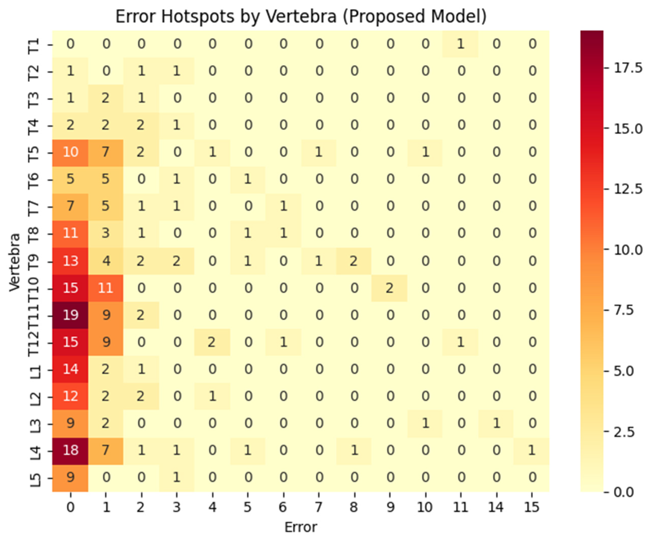
To further investigate the framework’s localization behavior, a vertebra-level error heatmap was generated by aggregating prediction errors across all anatomical levels from T1 to L5. Figure 4 visualizes this error distribution, measured in vertebral units, relative to the corresponding ground-truth landmarks.

As shown in Figure 4, prediction errors are highly concentrated within the 0 and ±1 vertebra columns across the entire spinal sequence. This pattern demonstrates that the majority of localization errors remain confined to adjacent vertebral levels and rarely deviate substantially from ground-truth positions.

The highest density of zero-error predictions spanned multiple vertebral regions, demonstrating the framework’s capability to accurately localize anatomical landmarks throughout the spinal column. Furthermore, the error distribution decayed rapidly as the magnitude of vertebral deviation increased, indicating that severe localization failures were exceptionally rare.

A slightly higher concentration of minor localization errors was observed near the thoracolumbar junction (T11–L1), where transitional curvature patterns often increase the ambiguity of vertebral landmark identification. Consistent with the landmark-wise results presented in Section 4.5, localization errors were generally larger for landmarks situated near gradual curve-transition regions than for the geometrically prominent apex vertebra.

Importantly, very few predictions fell within the large-error regions of the heatmap, demonstrating that the proposed framework rarely produces anatomically implausible vertebral assignments. This minimal occurrence of implausible predictions is consistent with the intended role of the anatomy- and geometry-guided learning constraints [25,29]. Overall, the observed error distribution validates the effectiveness of the proposed geometry-aware sequence learning strategy in maintaining structurally consistent landmark localization.

4.7. Comparison with CurvNet and Subsequent Spinal-AI2024-Based Studies

To clarify the methodological positioning of the proposed framework,

Table 16. Methodological comparison of studies utilizing the Spinal-AI2024 dataset.

Comparison Aspect	CurvNet [27]	SpineCheck [32]	Proposed Framework
Primary task	Cobb angle estimation and dataset curation	Vertebral segmentation and automated Cobb angle calculation	Scoliosis type classification and vertebral landmark localization
Main method	Latent contour representation, anchor-box classification, and iterative data processing engine	U-Net-based segmentation models and geometry-driven angle calculation	YOLOv8-OBB feature descriptors, 1D Residual CNN-BiLSTM architecture, and GeoLoss optimization
Use of Spinal-AI2024	Dataset curation, development, and evaluation	Evaluation on 20,000 images	Development set: 550 images; held-out test set: 58 images
Main output	Maximum Cobb angle and regional angles (PT, MT, TL/L)	Vertebral masks and Cobb angle quantification	Scoliosis curve type (C/S) and vertebral levels (UEV, LEV, AV)
Evaluation metrics	SMAPE	Dice coefficient, MAE, Pearson correlation coefficient, and ICC(A,1)	Type Accuracy, landmark Accuracy (±1 and ±2), and vertebral-level MAE

compares this work with CurvNet [27] and a subsequent study, SpineCheck [32], both of which utilize the Spinal-AI2024 dataset.

Because these studies address different target tasks and report distinct evaluation metrics, the comparison focuses on their research objectives, methodological designs, output formats, and evaluation strategies rather than presenting a direct numerical performance ranking.

CurvNet [27] introduced the Spinal-AI2024 dataset and formulated scoliosis assessment as a curvature-angle estimation problem utilizing latent contour representations, anchor-box classification, and an iterative data engine. Its evaluation focused on the maximum Cobb angle alongside regional angles across the proximal thoracic, main thoracic, and thoracolumbar/lumbar segments.

Subsequently, SpineCheck [32] leveraged the same dataset to develop an integrated vertebral segmentation and Cobb angle calculation platform. Their framework is based on multiple U-Net variants coupled with geometry-driven post-processing.

In contrast to prior works, the proposed framework does not directly regress or calculate Cobb angles. Instead, it addresses an intermediate but clinically vital task by explicitly predicting the scoliosis curve type and the vertebral levels for the UEV, LEV, and AV. The ordered vertebral sequence is defined by orientation, displacement, shape, confidence, and curvature descriptors, which are modeled using a 1D Residual CNN-BiLSTM architecture with geometric regularization.

Consequently, the proposed framework complements rather than directly replaces CurvNet and SpineCheck. It does so by shifting the research emphasis toward interpretable vertebral landmark selection and sequential anatomical modeling.

Because these studies differ significantly in their target outputs and evaluation metrics, their reported numerical results should not be interpreted as a direct performance ranking. CurvNet and SpineCheck measure errors in continuous Cobb angles, whereas this study evaluates errors across discrete vertebral levels.

To enable a direct quantitative comparison in the future, Cobb angles must be calculated using the UEV and LEV predicted by the proposed framework. These results can then be evaluated using the same angle-based metrics, including symmetric mean absolute percentage error (SMAPE), MAE, Pearson correlation coefficient, and intraclass correlation coefficient (ICC).

A limitation of the present study is that all experiments were conducted using the Spinal-AI2024 dataset, which consists of synthetic scoliosis radiographs. Although the disjoint held-out test set contained completely unseen images, these samples were drawn from the same source dataset and therefore evaluate same-source generalization rather than external clinical generalizability. An independent institutional dataset of real scoliosis radiographs with the required vertebral landmark annotations was not available for this study; consequently, external clinical validation could not be performed.

Future work will evaluate the frozen framework on real radiographs collected from independent institutions and, where possible, across multiple centers to assess its robustness to variations in image acquisition, image quality, and patient anatomy. Such external validation will be essential for determining whether the proposed method can generalize beyond the synthetic data used in the present study and for establishing its applicability in real clinical settings.

5. Conclusions

This study introduced a geometry-aware multi-task sequence learning framework for automated vertebral landmark localization and scoliosis type classification from coronal radiographs. YOLOv8-OBB detections were transformed into structured 12-dimensional geometric sequences and processed using a 1D Residual CNN-BiLSTM architecture. The proposed GeoLoss further incorporated displacement-based geometric information into the optimization process to improve the consistency of vertebral landmark localization.

The ablation study demonstrated the complementary contributions of local convolutional feature extraction, bidirectional sequence modeling, and geometry-aware optimization. Specifically, in the fourth experimental run using the 75/15/10 partition, incorporating GeoLoss into the 1D Residual CNN-BiLSTM framework increased EV Accuracy (±1) from 80.95% to 88.51% and EV Accuracy (±2) from 88.32% to 90.25%. Under the same configuration, the complete framework achieved a Type Accuracy of 97.22%.

Same-source generalization was further evaluated on a disjoint, held-out test set comprising 58 previously unseen images from the Spinal-AI2024 dataset. On this independent test cohort, the frozen model achieved an image-level Type Accuracy of 96.55%, an EV Accuracy (±1) of 86.63%, an EV Accuracy (±2) of 94.19%, and an EV MAE of 0.559 vertebral levels.

Overall, these findings support the potential of ordered vertebral geometry and bidirectional sequence modeling for automated scoliosis assessment. However, external validation using real clinical radiographs from independent institutions remains necessary to determine the generalizability of the framework across variations in image acquisition, image quality, and patient anatomy before its clinical applicability can be established.