1. Introduction
Nowadays, it is well established that plant diseases cause significant damage to crop yields, economic profits, and the quality of food and other products. Furthermore, incorrect classification of diseases leads to the use of inappropriate and ineffective treatment methods. Consequently, rapid and accurate disease classification, as well as the ability to diagnose plants individually rather than relying on statistical averages, are crucial for improving agricultural management and ensuring safety.
Recent improvements in machine learning have made the automation of the aforementioned task possible. Convolutional neural networks (CNNs) have demonstrated the ability to recognise plant diseases from leaf images and learn from image datasets without manual feature extraction, achieving over 99% accuracy on benchmark datasets under controlled conditions [
1,
2]. Subsequent research has explored various CNN architectures, including ResNet, DenseNet, and EfficientNet, consistently achieving high performance on laboratory data. More recently, Vision Transformers have been applied to plant disease classification, showing competitive or superior results compared to CNNs, particularly when trained on large-scale datasets [
3]. Recent hybrid approaches combining CNNs with Vision Transformers have further advanced the field. Dhruw et al. [
4] developed a unified CNN-ViT model for cotton disease and pest classification, achieving 98.5% accuracy by integrating local feature extraction with global context capture. Similarly, Aboelenin et al. [
5] proposed a hybrid framework combining ensemble CNNs with ViT for plant leaf disease detection, attaining 99.24% accuracy on apple and 98% on corn datasets.
However, the gap between controlled laboratory conditions and real-world agricultural environments remains a persistent challenge. Despite this success, approaches based on CNNs face some challenges. Many diseases have subtle texture variations, irregular lesion patterns, and multi-scale visual structures on leaf surfaces. It can be difficult for CNNs to capture these features effectively, especially when symptoms appear at different spatial scales. As a result, classification performance can degrade significantly when the visual patterns are highly heterogeneous or not strongly manifested.
The possibility of using machine learning in automatization of plant disease classification has been accurately studied by many researchers. The work [
6] represents an early development stage of methods for automatic plant disease recognition. It proposes an approach based on image segmentation using a genetic algorithm and Support Vector Machines or k-means classification methods. Early works were crucial for the development of plant disease automatic classification from images. Mohanty et al. [
1] were among the first to demonstrate the high potential of deep learning in plant pathology using the PlantVillage dataset, achieving accuracy of up to 99.35% in recognizing multiple disease classes using convolutional neural networks. Simultaneously, Sladojevic et al. [
2] have proposed a deep neural network architecture for classifying leaf diseases, confirming the effectiveness of this approach and laying the foundation for subsequent research. Both studies demonstrated the compelling applicability of CNNs to plant disease diagnosis. The study [
7] proposed one of the first fine-grained approaches, moving from classifying entire leaves to analyzing individual lesions and spots. This approach increased the diversity of the training set without collecting new images and improved classification accuracy by an average of 12% when working with 79 disease classes on 14 crops.
In addition to early successes, large-scale reviews have systematically assessed the current state of the field. A systematic review of the application of deep learning in agriculture is presented in [
8]. The authors identified the following areas: crop classification, weed detection, plant disease recognition, soil health assessment, and yield prediction. With regard to plant pathology, they noted that convolutional neural networks provide high accuracy but face a number of challenges: lack of processed data, sensitivity to lighting and background, and poor model interpretability. It was also noted that most studies are conducted on standard datasets (e.g., PlantVillage), and the transferability to real-world field conditions remains an unresolved challenge. The authors of the studies [
9,
10] reached similar conclusions regarding the effectiveness of CNNs and their limitations, including small datasets, the influence of image background, and the variability in disease symptoms. The paper [
10] also introduces the concept of “imperfect robustness,” referring to a drop in accuracy when the model is transferred to real-world field conditions. A review of methods for detecting and classifying plant diseases using deep learning, highlighting both the potential and limitations of modern approaches, is presented in [
11]. In [
12], the authors analyzed a wide range of machine learning and deep learning methods and concluded that CNNs demonstrate high accuracy on test data; however, their performance declines significantly in real-world conditions due to changes in lighting, background, and other factors.
The current state of the field has been recently consolidated in several systematic reviews [
13,
14], which have identified key challenges in model generalisation, dataset limitations, and the importance of robust feature extraction.
Apart from the variability of external conditions, another major challenge is the lack of data. Many plant diseases are rare or confined to specific geographic regions, making it difficult to collect sufficiently large and balanced training datasets. This problem is particularly acute for viral and parasitic diseases, which are underrepresented in open datasets. As a result, models trained on widely available data often perform poorly on rare disease classes. To address this problem, researchers employ data augmentation, synthetic image generation, and training on small samples; however, the challenge of generalizing to new disease patterns with a limited number of examples remains unresolved.
Recent studies have addressed the data scarcity problem through few-shot learning approaches. For instance, a transformer-based few-shot learning pipeline for barley disease detection was proposed in [
15], achieving 91.80% accuracy with as few as five images per class, while [
16] applied few-shot learning techniques to rice leaf disease stage classification using Siamese and prototypical networks.
Some studies have also been devoted to additional sensing methods for early disease detection. Specifically, hyperspectral imaging and spectral-signature analysis can reveal internal changes in plant leaves before visible symptoms appear. The study [
17] demonstrated that spectral analysis enables anticipatory detection of tomato fungal diseases. However, the widespread application of such methods is limited due to the need for specialized and expensive sensors. The study [
18] proposed the application of feature graphs to emphasize similarity between different diseases.
Feature extraction remains an important complement to any classification task and to the classification of plant diseases in particular. For example, a review of feature extraction methods [
19] shows that texture descriptors, color statistics, and morphological features can improve the performance of machine learning models. Manual features, such as local binary patterns (LBPs), gray-level co-occurrence matrices (GLCMs), and Gabor filters, were widely used in early plant disease detection systems and remain relevant, especially when dealing with small datasets. However, such features require careful tuning to specific conditions and often generalize poorly, especially when moving between different plant species.
Research on AI explainability to ensure transparency is presented in the paper [
20]. The authors proposed a neural network architecture that combines visualization and interpretability to accurately identify the regions of leaves that contribute most to the classification decision. As a result, model explainability can increase trust and promote personal use of automated diagnostic systems. A similar goal was pursued in [
21], which employed channel and spatial attention modules during training. Explainable AI is becoming increasingly important in agricultural applications, where experts need to understand why a model made a particular decision in order to trust it and act upon it. The importance of developing deep neural networks is demonstrated in [
22], where the authors make decisions ”for the right scientific reasons” when classifying plant diseases. Gradient-based visualization methods, such as Grad-CAM, LIME, and SHAP, have been applied to plant disease classifiers, providing heatmaps that highlight symptomatic areas [
23]. Recently, data-leakage-aware transfer learning combined with explainable AI was applied to the classification of mango leaf diseases [
24], demonstrating the practical value of XAI in agricultural diagnostics. However, these methods are typically post hoc and do not actively guide the training process itself. Some studies have focused on optimization to make models suitable for use on mobile devices and drones. In [
25], the authors succeeded in removing 75% of the parameters with minimal loss of accuracy. A recent study [
26] also demonstrated that lightweight deep learning models can achieve high accuracy in detecting potato diseases, making them suitable for deployment on edge devices.
Our most important area of research involves the application of fractal analysis to describe complex natural textures. At the present stage, the theory of self-organization represents a promising field that is actively used to study objects, processes, and phenomena that exhibit self-similarity and a high degree of self-order or, conversely, possess properties such as dissipativity, irregularity, roughness, chaos, and disorder. Concepts from fractal theory often serve as the theoretical basis for the mathematical formalization and quantitative analysis of self-organizing objects [
27]. Since a key feature of fractals is the self-similarity of their structure across different scales, fractal theory has found widespread application in condensed matter physics for the analysis of solid-state structures. The central concept of fractal theory is fractal dimension. Complex physical systems are characterized by the manifestation of self-similarity across a hierarchy of scale levels; therefore, a set or spectrum of dimensions is used to describe such objects—multifractals. The main approach in applying fractal and multifractal analysis methods consists of establishing relationships between the physical properties of an object and the scaling characteristics of its self-similar structure or dynamic behavior. Multifractal parameterization algorithms play a particularly important role in practice as tools for detailed analysis of the dispersion of fractal dimensions, which characterize the statistical properties of heterogeneous self-similar structures [
28].
Fractal geometry has been successfully used to characterize irregular, self-similar structures in biological and medical images. In medical diagnostics, fractal analysis has been applied to skin lesions, retinal images, and histopathological slides, showing that fractal descriptors can capture subtle morphological changes indicative of pathology. In modern scientific literature, one of the most important tasks for which multifractal analysis methods can be applied is the problem of the processing, characterization, and classification of complex 2D and 3D raster images and structures. Examples of such applications are widely described in the literature and represented by interdisciplinary research in materials science, chemistry, meteorology, geodesy, hydrology, biology, medicine, and other fields [
29,
30,
31].
Fractal descriptors have been successfully applied to plant disease classification in [
32]. The authors have shown that fractals can effectively characterize irregular lesion patterns on leaves, although this analysis was used solely for interpreting the already trained model and remains a post hoc tool.
Among the methods of multifractal analysis of two-dimensional structures and raster images, methods based on covering the object with clusters deserve special attention, in which the number of ”occupied” clusters is counted as their size decreases, as well as their specific weight. Methods of this group are based on the earlier idea of the covering method or “box-counting” [
33]. These methods, for example, have been applied to the analysis of binarized and grayscale raster images of objects of various nature.
Another promising and continuously developing direction is the use of wavelet transforms for estimating multifractal characteristics of images. The method of wavelet transform modulus maxima (WTMM), proposed by Muzy, Bacry, and Arneodo [
34,
35], has found application for calculating the scaling characteristics of two-dimensional raster images and has been extended to 3D fields [
36]. Alternative approaches include wavelet-based multifractal detrended fluctuation analysis and the wavelet leader method [
31,
37], which has been further developed for texture classification. In particular, multifractal wavelet analysis has demonstrated its effectiveness in medical image diagnostics, where fractal features extracted via wavelet transform provide robust biomarkers for early diagnosis of pathologies such as glaucoma [
38]. The applicability of this approach to processing self-similar structures in raster images has been further developed in the context of multifractal wavelet analysis algorithms [
39].
It should be noted that the proposed use of WTMM-based fractal descriptors is not limited to the simple construction of features. The descriptors act as a structured regularizer that introduces a mathematically sound inductive bias into the training process of a convolutional neural network. Unlike data-driven approaches, which must independently detect relevant textural patterns, WTMM descriptors encode mathematical a prioriknowledge about the multiscale self-similarity of diseased tissue. This prior knowledge guides the network toward physically meaningful characteristics, such as irregular lesion boundaries, scale-invariant textural variations, and heterogeneous spatial structures. As a result, the network is less likely to explore arbitrary decision surfaces based on limited data. The fractal formalism facilitates decision-making “based on sound scientific reasoning” [
22], as it shifts the feature space toward diagnostically significant morphological properties.
The fractal attention module (FAM) extends this idea by using precomputed mathematical texture characteristics to guide spatial attention. This approach differs from conventional data-driven attention mechanisms, which must learn spatial relevance entirely from labelled examples. By anchoring attention in an explicit texture model, the FAM reduces the sample complexity required to determine where to focus and offers a more interpretable foundation for spatial weighting. This structured regularization proves particularly beneficial in low-data regimes, where purely data-driven mechanisms are prone to overfitting, and it helps account for the rapid convergence and improved robustness observed in our experiments.
Despite the results achieved, most existing approaches either rely exclusively on deep neural networks or use hand-crafted descriptors as features. The potential for integrating fractal texture analysis directly into convolutional neural networks remains relatively unexplored. Multiscale fractal descriptors can be useful for describing scale-invariant and self-similar properties of complex biological textures. Thus, there is a gap between classical fractal texture analysis and modern deep learning approaches to plant disease classification. Although post hoc fractal analysis has been shown to correlate with disease severity, none of the existing studies integrate fractal descriptors as an inductive bias during CNN training to actively guide feature extraction and enhance model robustness.
In this work, we overcome the limitations listed above by proposing a pipeline for extracting multifractal features and integrating the resulting descriptors directly with convolutional neural networks to improve texture representation and enhance classification robustness. In the context of plant pathology, leaf lesion patterns often exhibit irregular geometric structures that can be effectively characterized using the described method.
The main achievements, including contributions to the field, can be summarized as follows: we propose a method for extracting multi-scale fractal maps based on the wavelet transform modulus maxima (WTMM), which produces two complementary descriptors, fractal dimension and singularity spectrum width, from leaf images at multiple spatial scales. We also introduce the fractal attention module (FAM), an architectural component that uses fractal maps as a modulating signal to emphasize discriminative spatial regions within a ResNet-50 backbone. We further design a combined training scheme, where fractal descriptors are used both for spatial attention and as a global embedding vector, complementing the conventional RGB feature stream. Finally, we provide interpretable attention maps that offer spatial explanations of the model’s decisions, contributing to the transparency of automated plant disease diagnosis.
The remainder of this paper is organized as follows.
Section 2 describes the proposed framework, including the task definition, the multi-scale fractal analysis via wavelet transform modulus maxima (WTMM), the fractal map generation procedure, the fractal attention module (FAM), the experimental dataset collection and preprocessing, and the implementation details of the training pipeline.
Section 3 presents the baseline models, evaluation metrics, experimental results with fractal maps on truncated datasets, and robustness analysis on corrupted test sets.
Section 4 discusses the implications of the obtained results, including convergence dynamics, the role of the attention mechanism, and interpretability aspects.
Section 5 outlines the limitations of the current approach and suggests directions for future work.
Section 6 concludes the paper with a summary of the main findings and their potential impact.
2. Proposed Framework
2.1. Problem Formulation
Let us formulate the plant disease classification task. We consider it as a supervised learning problem. The input is a set of RGB images represented as tensors:
where
H and
W denote the height and width of the image, respectively.
In order to focus on the diversity of diseases rather than on fine-grained distinctions between individual pathologies, we group all pathologies into five broad classes according to the type of causative agent: bacteria, fungi, healthy, parasites, and viruses. This grouping is motivated by the fact that treatment strategies differ fundamentally between these groups, and misdiagnosis at this level has direct practical consequences.
The proposed pipeline was developed for pathogen-type classification as a first-level screening tool. This grouping was adopted for the low-data regimes investigated in this study, where fine-grained discrimination between individual diseases of the same pathogen type is often unreliable. It should be emphasised that the proposed methodology is not limited to this coarse taxonomy. The multi-scale fractal feature extraction and the fractal attention module can be directly applied to fine-grained classification tasks, including specific diseases of specific crops, by retraining the model on the corresponding labelled data. For practical agricultural deployment, the same approach can be adapted to any desired disease taxonomy.
Formally, the set of labels is
corresponding to the five classes listed above. The goal is to train a classifier
that maps an input image to its correct class, minimizing classification error on unseen data.
This grouping has certain limitations. It loses fine-grained distinctions between pathogen species and does not account for mixed infections. Cases caused by oomycetes, such as late blight, were excluded, as these organisms are taxonomically distinct from true fungi but produce similar symptoms. Images with ambiguous etiology, such as unspecified leaf blight, were also excluded.
The label mapping was performed manually by a domain expert based on the pathogen etiology reported in each dataset. For instance, powdery mildew and rust were assigned to fungi, bacterial spot to bacteria, and mosaic virus to viruses. The complete preprocessing pipeline, including the filtering and mapping logic, is available in the GitHub (version 1.0.0) repository referenced in the Data Availability Statement.
2.2. Fractal Feature Extraction via Wavelet Transform Modulus Maxima
Given the multi-scale and self-similar properties of leaf disease patterns, we employ the wavelet transform modulus maxima (WTMM) method. This approach was chosen over conventional fractal descriptors, such as box-counting, for several reasons. Box-counting is sensitive to the choice of grid and performs poorly on irregular, sparse patterns that are typical of disease lesions. It also provides only a single global fractal dimension, which does not reflect the heterogeneity of textures at different scales. In contrast, WTMM yields a rich multifractal spectrum that captures both the global scaling behaviour and local singularities, making it particularly suitable for analysing the complex, multi-scale visual structures found in diseased plant leaves.
For an image
in grayscale, where
denotes the spatial coordinates, the wavelet transform at scale
is defined as
where
is the integration variable over the image domain and
is a wavelet-like operator (in this work, we use the first derivative of a Gaussian,
gaus1).
The WTMM method then identifies points where the modulus of the wavelet transform is locally maximal at each scale. These points form scale-dependent ridge structures that localize the singularities of the image and provide a robust representation of its irregular structures.
These ridge structures are curves in the scale-space domain that connect local maxima of the wavelet transform modulus across scales. They localise singularities such as edges, corners, or irregular texture boundaries. The ridge structures themselves are intermediate mathematical objects and are not directly visualised in the final fractal maps; instead, the maps are derived from these ridges through the multifractal formalism described above.
From these maxima, the partition function is computed as
where the sum runs over the local maxima at scale
s, indexed by
i. For a given moment order
, the scaling exponent
is obtained from the power–law relation
which holds in the limit of small scales, where the multifractal scaling behaviour dominates.
The singularity (Hölder) exponent
h and the multifractal spectrum
are then derived via the Legendre transform:
The spectrum
describes the distribution of singularities in the image, with
h characterising the local regularity of the signal.
In this work, we focus on two WTMM-derived descriptors that are particularly relevant for plant disease analysis:
(1) Fractal dimension , which corresponds to the dimension of the singularity support and characterizes the global complexity of the lesion texture;
(2) Spectrum width , which quantifies the heterogeneity of the texture by capturing the diversity of local structures across scales. This descriptor is useful for distinguishing between different types of tissue damage, as lesions with high heterogeneity tend to have broader spectra.
2.3. Multi-Scale Fractal Map Generation
The WTMM descriptors introduced in the previous subsection are local features that characterise the fractal properties of an image. To capture spatial variations in these properties across the image, we compute the descriptors locally for each image region and generate spatial maps of fractal dimension and spectrum width. We perform this procedure at three spatial scales with patch sizes .
The specific values were selected through a hyperparameter search using Optuna on a validation subset, with the search space covering values from 32 to 128 pixels and the objective of maximizing validation accuracy on the 50-shot setting. This triplet balances fine-grained lesion detail at the smallest scale, intermediate texture patterns at the middle scale, and global structural organization at the largest scale. Patch sizes below 64 pixels produced unstable estimates of the multifractal spectrum due to insufficient statistical samples for the partition function.
Boundary conditions are handled by adaptive non-overlapping grid partitioning. For each scale s, the number of cells is (with a minimum of 1), and cell boundaries are computed by evenly splitting the range using integer arithmetic . This ensures full coverage without padding or cropping; individual cell sizes may differ by at most one pixel. Overlapping patches or smaller step sizes were not adopted, as the computational cost of WTMM computation scales quadratically with the number of patches, and preliminary experiments showed only marginal improvements (less than 1.5% in validation accuracy) that did not justify the additional cost.
The complete set of WTMM extraction parameters is summarised in
Table 1.
The chosen scales balance representational richness and computational cost: the smallest scale captures fine-grained lesion details, the middle scale reflects intermediate texture patterns, and the largest scale characterises global structural organisation. A smaller number of scales would oversimplify the multi-scale nature of disease textures, while a larger number would increase computational overhead without proportional improvement.
For each scale s, the map generation proceeds as follows:
(1) The input image of size is divided into a grid of non-overlapping patches of size ;
(2) For each patch, the fractal dimension and spectrum width are computed using the WTMM framework described in the previous subsection. The moment order q is sampled in the range with 5 steps, which provides a sufficient resolution of the multifractal spectrum while keeping the computation tractable;
(3) The resulting low-resolution maps are bilinearly upsampled to the original resolution , producing two full-size maps per scale: and .
All maps are then concatenated into a multi-scale fractal tensor:
Each channel is normalised independently to the range
. The resulting tensor encodes both the fractal dimension and textural heterogeneity at multiple scales, providing complementary information to the RGB image. Note that the parameter selection, including the scales and
q-range, is flexible and can be adjusted for different datasets or applications.
2.4. Fractal Attention Module
The multi-scale fractal tensor M generated in the previous step serves as an auxiliary feature representation. We introduce the fractal attention module (FAM), which learns to emphasise spatial regions where fractal properties are most discriminative for disease classification.
The FAM is implemented as a lightweight convolutional subnetwork:
where
denotes the sigmoid function. This architecture was chosen for two reasons. First, the
convolution captures local spatial context from the fractal tensor, while the subsequent
convolution aggregates this information into a single-channel attention map. Second, the sigmoid activation ensures that the output
can be interpreted as a spatial weighting mask.
During the forward pass, the fractal tensor
M is resized to match the spatial dimensions of the feature map
F produced by the third stage of the ResNet-50 backbone. We chose this insertion point because the third stage provides a sufficiently high-level feature representation while preserving enough spatial resolution for meaningful attention modulation. The attention map is then applied as
where
is a trainable scalar parameter initialised to a small value (e.g.,
). The initial value of
was set to 0.01 based on preliminary experiments and further tuned within the Optuna hyperparameter search. The term
allows the network to both suppress (
) and amplify (
) features based on local fractal properties, rather than simply scaling them. This provides greater flexibility than a standard multiplicative attention.
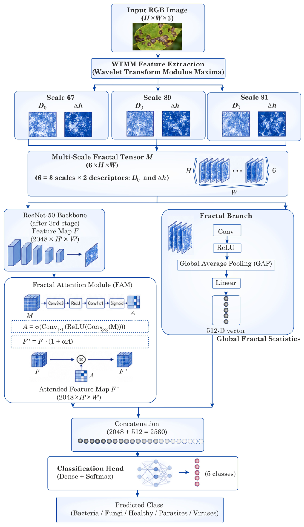
In addition to spatial attention, the fractal tensor M is passed through a separate encoder consisting of a convolutional layer, ReLU activation, global average pooling, and a linear layer. This produces a compact fractal embedding vector that captures global fractal statistics. The embedding is concatenated with the ResNet-50 feature vector before the final classification layer. The combined architecture, which integrates both the attention mechanism and global embedding, is called FractalResNet.
It should be emphasised that the RGB stream and the fractal stream are not independent. The ResNet-50 backbone processes the RGB image as its primary input. The fractal tensor is computed separately and used in two ways: as a modulating signal in the FAM, which is inserted after the third stage of ResNet-50, and as input to a separate encoder producing a global fractal embedding. The FAM modulates the intermediate feature maps of ResNet-50, while the global embedding is concatenated with the backbone features before the final classification layer. Thus, the fractal information is injected into the pretrained backbone at an intermediate stage rather than being concatenated at the input.
The overall architecture is illustrated in
Figure 1.
The input RGB image is processed through the WTMM-based fractal feature extraction pipeline to produce a multi-scale fractal tensor M. This tensor is used in two ways: as a modulating signal in the fractal attention module (FAM) applied to the ResNet-50 feature map, and as input to a separate encoder that produces a global fractal embedding vector. Both the attention-modulated features and the fractal embedding are concatenated and passed to the classification head.
2.5. Experimental Setup
We compiled a heterogeneous collection of 11 publicly available plant disease datasets, including PlantVillage [
40], Wheat [
41], PlantDoc [
42], Cotton [
43], Rice [
44], Pea [
45], Sugarcane [
46], and Lemon [
47]. The images were grouped into five categories according to pathogen type: bacteria, fungi, healthy, parasites, and viruses. In the original datasets, the labels typically correspond to specific diseases rather than pathogen classes; we manually mapped the labels and excluded images with uncertain pathogen etiology, such as late blight caused by oomycetes.
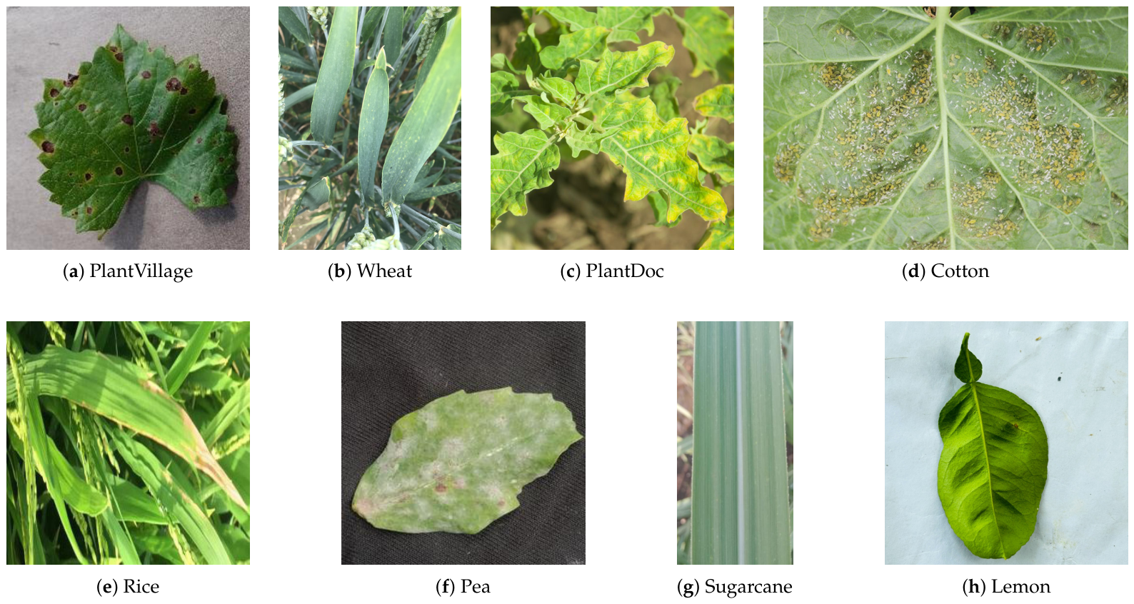
Figure 2 shows representative samples from the main datasets used in this work. The collection includes PlantVillage, a standard benchmark with controlled lighting and uniform backgrounds; Wheat, which contains images acquired under complex field conditions; PlantDoc, which covers multiple species with varying backgrounds; and several other datasets covering cotton, rice, pea, sugarcane, lemon, and other crops. In total, the combined dataset comprises 358,751 images.
The dataset covers multiple crop types, including potato, tomato, wheat, cotton, rice, pea, sugarcane, and lemon. The class distribution across the five pathogen types is as follows: bacteria—101,237 (28.22%), fungi—84,755 (23.63%), healthy—74,631 (20.80%), parasites—53,896 (15.02%), and viruses—44,232 (12.33%). The test set is held out separately with the following distribution: bacteria—1087, fungi—741, healthy—881, parasites—242, viruses—123.
The training, validation, and test split is performed by reserving 1% of images from each class as a held-out test set. The remaining data are split into training and validation sets with a validation ratio of 0.1 (at least one image per class is kept for validation). The class imbalance is addressed using WeightedRandomSampler with weights inversely proportional to class frequencies, focal loss with class weights, and Mixup augmentation. Stratified splitting preserves class proportions during validation. The full dataset structure is available in the GitHub repository.
Preprocessing was performed using a custom script. The pipeline includes conversion of all images to JPEG format, extraction of 1% of training images per class to form a held-out test set, file renaming to a unified format, deduplication, and removal of empty directories. The remaining data were split into validation and training sets (10% and 90%, respectively). The dataset structure and preprocessing code are available in our GitHub repository.
2.6. Implementation Details
We use a ResNet-50 backbone pretrained on ImageNet as the main image encoder. When the fractal branch is enabled, the model receives the RGB image along with a multi-scale WTMM tensor with channels, where and the scales are . We refer to this combined architecture as FractalResNet.
The fractal tensor is computed from a grayscale representation (default: LAB luminance channel). The WTMM extraction parameters include the wavelet type (gaus1, gaus2, or mexh), the maxima percentile threshold, the ridge radius, and the q-range sampled in wtmm_q_steps points. For each scale, the pipeline produces two full-resolution maps, the fractal dimension and the spectrum width , each normalised to .
The fractal attention module is applied after the third stage of the ResNet-50 backbone, as described in the previous subsection.
To handle class imbalance (bacterial and fungal diseases are significantly more frequent than viral and parasitic ones), we use a
WeightedRandomSampler with weights
where
N is the total number of training samples,
is the frequency of class
, and
C is the number of classes. Class weights are also incorporated into the loss function. We use focal loss with class weights computed from the training split.
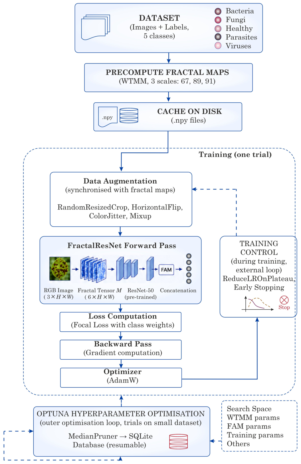
Images are resized to (configurable via the –img_size parameter). The training pipeline applies RandomResizedCrop, RandomHorizontalFlip, and ColorJitter augmentations, which are synchronised with the corresponding fractal maps. Mixup augmentation is also applied. Optimisation is performed with AdamW; the learning rate is scheduled using ReduceLROnPlateau on the validation loss with patience 3 and factor 0.5. Early stopping is enabled with patience 5 and a minimum improvement threshold of .
WTMM maps are precomputed and cached on disk to avoid recomputation during training. The pipeline supports precomputation via the –precompute_fractal flag, which saves maps as .npy files with a configuration-dependent name. The dataset class loads the cached maps during training and falls back to a zero tensor if a map is missing.
Hyperparameter tuning for the fractal branch is performed using Optuna. Each trial runs a full training cycle on a small subset of the data and evaluates the resulting model on the validation set. A MedianPruner terminates clearly unpromising trials early. The optimisation study is stored in a persistent SQLite database, allowing it to be resumed.
Figure 3 illustrates the complete training pipeline, including data loading, fractal map precomputation and caching, synchronised augmentation, forward and backward passes, loss computation, and hyperparameter optimisation.
4. Discussion
The experimental results indicate that the proposed fractal branch acts not as a mere supplementary input, but as a mechanism that modifies the learning dynamics and spatial attention of the network. On the truncated datasets, the model with fractal maps outperformed the RGB-only baseline: accuracy increased from 57.06% to 67.73% on the 5-shot setting, and from 80.81% to 86.11% on the 50-shot setting. The same trend was observed under corrupted-test conditions, where the fractal-augmented models achieved higher average accuracy in both settings. These results suggest that fractal descriptors contribute to both classification performance and robustness under perturbations affecting colour, local structure, or background statistics.
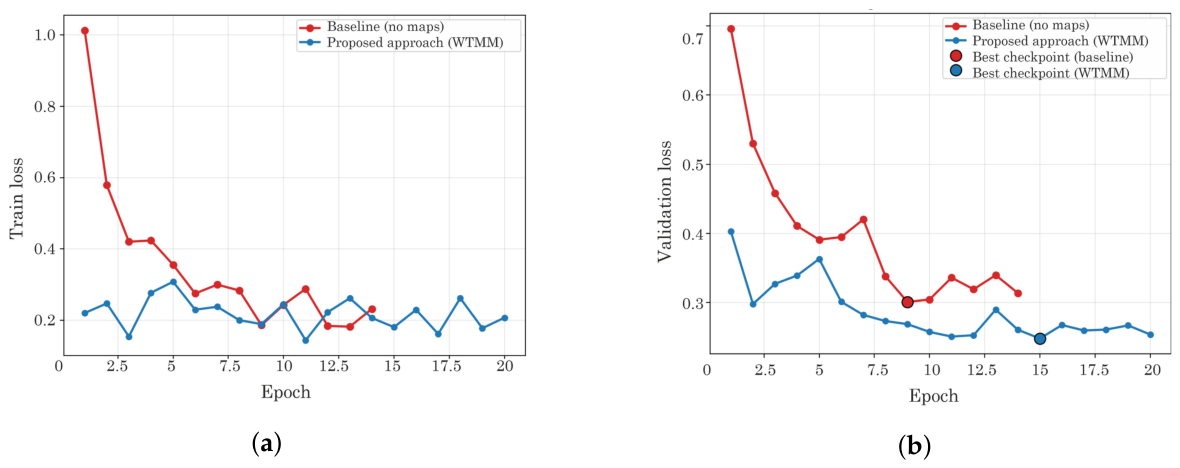
The convergence behaviour differs markedly between the two models. The baseline required 25–40 epochs before early stopping, whereas the fractal-augmented model reached its final validation accuracy within 1–2 epochs. We acknowledge that a rigorous statistical evaluation of the convergence behaviour with multiple independent runs would strengthen this claim. However, the convergence curves presented in
Figure 4 show that the fractal-augmented model reaches a validation loss plateau within the first one–two epochs across all experimental settings. This behaviour was stable across multiple runs. The rapid convergence is a direct consequence of the strong inductive bias provided by the fractal descriptors, which is consistent with the theoretical expectation. A systematic statistical evaluation of convergence dynamics remains an interesting direction for future work.
It should be clarified that the rapid convergence refers to validation accuracy reaching a plateau within one–two epochs, while the validation loss continues to decrease more gradually. This is consistent with the behaviour observed in
Figure 4, where the loss reaches 0.10 by epoch 13. The key point is that the fractal-augmented model reaches its final accuracy level substantially faster than the baseline, which requires 25–40 epochs.
After that, training continued for approximately five additional epochs without meaningful improvement before termination (early stopping patience = 5). This behaviour indicates that the fractal branch provides a strong inductive bias that helps the backbone separate classes much earlier in training. The maps do not simply add extra channels; they make the discriminative structure more accessible from the outset.
The rapid convergence observed for the fractal-augmented model warrants further discussion. It does not imply that the backbone layers remain frozen; gradients still update the ResNet-50 weights during training. However, the fractal prior provides a strong inductive bias that simplifies the classification problem from the outset, which is why the final layers dominate the initial loss reduction. The backbone is not bypassed; rather, it is guided toward discriminative texture features more efficiently.
We acknowledge that overfitting remains a potential concern, particularly in highly heterogeneous or out-of-distribution field conditions, where fixed WTMM parameters may become suboptimal. This risk is mitigated by several factors: the RGB stream continues to learn complementary appearance-based features, strong augmentations (MixUp, ColorJitter, RandomResizedCrop) are applied during training, and the robustness experiments demonstrate that fractal-augmented models generalise better than baselines under various corruptions. Nevertheless, systematic evaluation on diverse external datasets is needed to fully assess generalisation, and we have noted this as a direction for future work.
The method should not be misinterpreted as a replacement for large-scale training. The fractal approach is best understood as a complementary mechanism. The fractal attention module (FAM) is central to this behaviour. The FAM does not replace the original image stream or learn a second full backbone from scratch. Instead, it injects fractal information at an intermediate feature level, after the third ResNet stage, where representations are already abstract enough for spatial modulation to be meaningful. This design choice is important. If the fractal maps were simply concatenated to the RGB input, the first convolutional layer would need to learn how to combine two modalities with very different statistics, partially negating the benefit of ImageNet pretraining. The FAM avoids this issue by treating fractal descriptors as a modulation signal rather than raw input.
The compressed nature of the FAM is intentional and not a weakness. The attention map is reduced to a single spatial mask, because its purpose is not to preserve every fractal detail, but to determine where the backbone should trust its features more or less. The global fractal encoder retains complementary information in vector form, while the FAM handles local spatial emphasis. Together, these two branches provide a two-level use of fractal information: local attention and global statistical representation. This separation of function makes the architecture more expressive than simple concatenation.
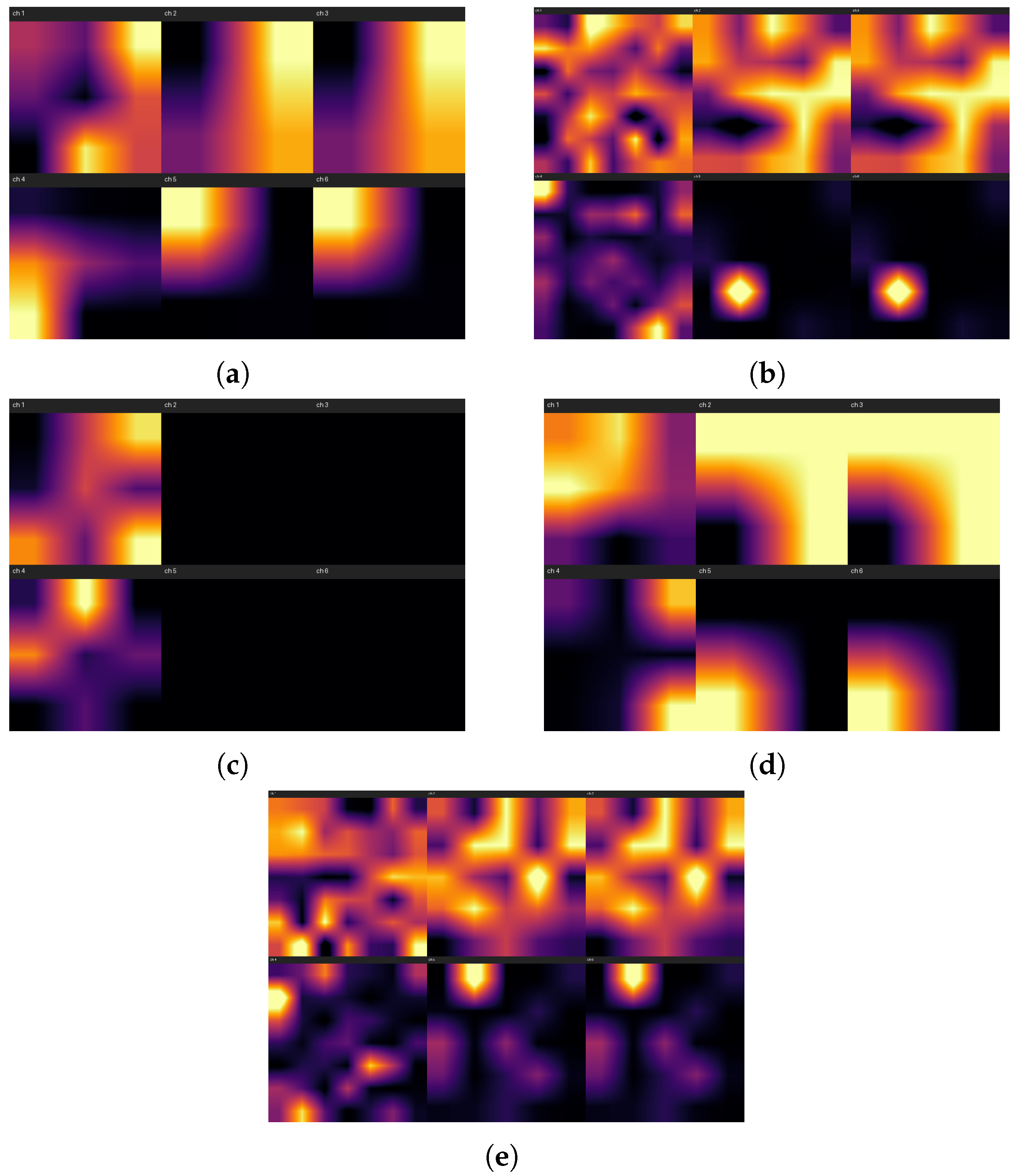
Another advantage of the FAM is interpretability. The module produces a spatial attention map that can be visualised and interpreted as a region-level explanation of the prediction. This is particularly valuable in plant disease analysis, where it is important to know whether the classifier focuses on symptomatic lesions, damaged edges, or background regions. The attention maps thus serve as a practical explainability tool, making the decision process more transparent than in a standard CNN pipeline. The fractal branch therefore provides not only improved learning dynamics, but also an interpretable bridge between fractal texture analysis and the final disease label.
The robustness experiments support this interpretation. On corrupted test variants such as grayscale conversion, random occlusions, and colour-channel removal, the fractal-augmented models were less sensitive than the baseline. This suggests that fractal descriptors capture structural properties that remain informative even when colour information is degraded. This behaviour is consistent with the observation that disease symptoms are defined not only by pigment changes, but also by irregular geometric organisation, boundary roughness, and multiscale texture variations. Fractal descriptors thus provide a complementary signal that is less dependent on the specific appearance of the image.
Overall, the experiments show that multi-scale fractal maps are most effective when treated as an auxiliary representation inside the network rather than as an additional input. This design yields faster convergence, better robustness, and a natural explanation mechanism, while preserving the strengths of the pretrained CNN backbone.
The scalability of the WTMM precomputation pipeline warrants discussion. The asymptotic complexity is , where N is the number of images, K is the number of scales, and M is the number of patches per image. For the full dataset of 358,751 images, three scales, and typical patch counts, the precomputation would require approximately 2.5 TB of storage and 200–300 GPU-hours on an A100. While this is acceptable for offline training in a research setting, it was beyond the practical constraints of this study.
Importantly, the full-dataset baseline already achieves 97.59% accuracy, confirming that the classification problem is highly learnable with abundant RGB data. The primary contribution of the fractal approach lies not in competing with large-scale training, but in improving learning efficiency, convergence speed, and robustness in low-data regimes. This is precisely where the method offers the greatest practical value, as agricultural datasets are often limited and heterogeneous.
A detailed ablation study isolating the individual contributions of the FAM and the global embedding branch was not performed, as the current implementation integrates these components as a unified architecture, and isolating them would require substantial code refactoring. Nevertheless, we can qualitatively discuss their expected roles. The FAM provides local spatial attention that emphasises regions where fractal properties are most discriminative, while the global embedding branch captures complementary statistical information about the overall fractal characteristics of the image. Both components are designed to work synergistically: the FAM modulates spatial features, and the global embedding enriches the final classification vector.
The complete FractalResNet outperforms the plain ResNet-50 baseline by 5.30% on the 50-shot setting (86.11% vs. 80.81%), demonstrating the effectiveness of the proposed approach as a whole. The ablation analysis remains an interesting direction for future work.
5. Limitations and Future Works
The proposed method has several limitations. The most significant of these is the computational cost of generating fractal maps. Although this is acceptable for offline training, the inference for a single image can take up to one minute on a typical mobile processor, which limits its applicability in real-time scenarios. Future work could explore simplified approximations of the WTMM algorithm or distilling the fractal feature extractor into a smaller network.
The parameter space of the WTMM pipeline, including the choice of wavelet basis, the number of scales, and the q-range, has been only partially explored. In particular, the proximity of patch sizes 89 and 91 suggests that a simpler configuration with two scales (e.g., 67 and 91) could be sufficient, possibly with a larger weight assigned to the larger scale. A systematic exploration of the number and values of scales remains an interesting direction for future work. A more systematic search could yield further improvements. The FAM architecture could also be extended; more sophisticated attention mechanisms, such as multi-head or deformable attention, could replace the current convolutional design. Integrating fractal maps with other modalities, such as hyperspectral or thermal data, could improve early disease detection. Although we have provided high-quality attention maps, a formal assessment of explainability, for example, using perturbation-based metrics would strengthen claims regarding interpretability.
In addition to the main method, the approach could benefit from evaluation on a broader range of datasets, including those with more severe class imbalances or diseases from different geographic regions. Extending the framework to multiclass classification or severity classification would also broaden its applicability. Finally, the proposed fractal feature extraction and attention mechanism are not task-specific. They can be transferred to other tasks involving irregular multiscale textures, such as medical image analysis, materials science, or remote sensing.
Evaluation on fine-grained classification tasks, where each disease of each crop is treated as a separate class, remains an important direction for future work. As noted in
Section 2.1, the proposed methodology is not limited to five classes and can be directly extended to such settings by retraining the model on the corresponding labelled data.
The robustness evaluation could be extended to include more realistic corruptions, such as directional lighting variations (e.g., adding gradient maps to simulate light coming from a particular direction), which would better reflect field conditions.
Overall, this work lays the groundwork for integrating fractal analysis into deep learning pipelines. The limitations are outweighed by the clear improvements in convergence speed, accuracy, and robustness that the method provides under conditions of limited and noisy data.
6. Conclusions
In this study, we proposed a multi-scale fractal feature extraction method for CNN-based plant disease classification. The method is built around the wavelet transform modulus maxima, which extracts two complementary descriptors—fractal dimension and singularity spectrum width—from leaf images at multiple spatial scales. These descriptors form six-channel fractal maps that are fed into a fractal attention module inserted after the third stage of a ResNet-50 backbone. A separate branch encodes global fractal statistics into an embedding vector. The two branches are combined at the classification stage, and the overall architecture is referred to as FractalResNet.
The experiments were conducted on a heterogeneous collection of 11 plant disease datasets under 5-shot, 50-shot, and full-scale training regimes. On the 5-shot setting, the fractal-augmented model improved accuracy from 57.06% to 67.73%; on the 50-shot setting, from 80.81% to 86.11%. The model also converged substantially faster: it reached final validation accuracy within 1–2 epochs, whereas the baseline required 25–40 epochs. Under corrupted test conditions, including grayscale conversion, random occlusions, and colour-channel removal, the fractal-augmented model generally outperformed the baseline, confirming that fractal descriptors capture structural information that is less dependent on colour and appearance.
The fractal attention module provides an additional benefit: interpretability. The attention maps it produces offer spatially explicit explanations of the model’s predictions, which is particularly valuable for agricultural applications where trust and transparency are important. The fractal approach should not be viewed as a replacement for large-scale RGB training. The highest raw accuracy was achieved on the full dataset (97.59%), confirming that abundant data remains the most direct path to high performance. Instead, the method is best understood as a complementary mechanism that improves convergence speed, feature extraction in low-data regimes, and robustness under noisy inputs.
Future work could explore several concrete pathways to address the inference bottleneck. First, GPU-accelerated parallel execution of the 2D WTMM algorithm could substantially reduce computation time. Second, depthwise separable convolutional approximations of the wavelet filters could provide a lightweight alternative with lower computational cost. Third, training a lightweight student network to directly predict WTMM maps from raw RGB inputs via knowledge distillation could bypass the expensive precomputation altogether.
In addition, more expressive attention designs and evaluation on a wider range of datasets remain interesting directions. Extending the framework to multi-label or severity-level classification would also broaden its applicability. Overall, this work demonstrates that fractal analysis can be effectively integrated into modern CNN pipelines, providing an efficient and interpretable inductive bias for plant disease classification.