NeuroFATE-MS: Privacy-Aware Federated Temporal Learning for Short-Term Multiple Sclerosis Progression Prediction

Abstract

Predicting short-term progression in multiple sclerosis (MS) from longitudinal clinical data remains challenging because visits occur at irregular intervals, patient trajectories vary substantially, and simulated federated clients often exhibit non-IID data distributions. Privacy constraints further limit centralized data aggregation, reducing the suitability of conventional temporal prediction models. We propose a federated learning framework for MS progression prediction that combines local and global temporal modeling with client-level imbalance handling under simulated privacy-preserving federated constraints. The model uses a bidirectional LSTM to capture short-range temporal dynamics and a Transformer encoder to model longer-range dependencies in irregularly sampled sequences. A cross-attention mechanism fuses these representations. Each client applies conditional trajectory augmentation with ProxiWGANP and a proximity constraint. Training uses federated averaging with gradient clipping and Gaussian noise injection, while privacy loss is estimated through Rényi differential privacy accounting. We evaluated the framework on a single-center longitudinal cohort of 517 patients and 4184 visits. After excluding first visits without historical context and visits without determinable 6-month follow-up labels, we derived 3184 eligible prediction windows. We partitioned these windows into 10 simulated federated clients using Dirichlet sampling and evaluated performance with a strict within-patient temporal split. Across five independent training seeds, the proposed method achieved a mean AUROC of 0.930 with a standard deviation of 0.003 and a mean AUPRC of 0.513 with a standard deviation of 0.005. For the primary seed, patient-level bootstrap estimates were AUROC 0.930 (95% CI: 0.912–0.948), AUPRC 0.515 (95% CI: 0.490–0.540), and ECE 0.014. These results suggest that the proposed framework can support accurate short-term MS progression prediction in a simulated federated setting. However, because the evaluation used a single-center cohort and simulated federation, the findings provide methodological evidence and require external multi-center validation before clinical deployment.

1. Introduction

Accurate prediction of short-term progression in multiple sclerosis (MS) from longitudinal clinical data is constrained by a combination of structural and statistical challenges that do not arise in standard supervised learning settings. Clinical trajectories are irregularly sampled, with visit intervals ranging from weeks to months, and missing observations are common due to inconsistent follow-up and modality-specific availability. Progression events are relatively infrequent and clinically heterogeneous, with labels defined through composite criteria such as relapse occurrence or sustained EDSS change, introducing both class imbalance and label uncertainty.

In real deployment settings, MS clinical data are often distributed across institutions and cannot be centrally aggregated because of data governance and privacy requirements. In this study, that constraint is approximated through simulated federated partitions derived from a single-center cohort. Federated learning (FL) enables decentralized training by aggregating model updates rather than raw data [1], but its optimization dynamics degrade under non-IID client data. In MS cohorts, non-IID effects arise from differences in patient populations, treatment strategies, and visit frequency, causing client drift and reduced convergence stability under standard FedAvg when minority-class events are unevenly distributed.

Temporal modeling in this setting requires representation consistency under irregular sampling. Recurrent models capture short-range dependencies but compress long-range information through sequential updates [2]. Attention-based models improve global context modeling [3] but are sensitive to missing or unevenly spaced observations. In federated settings, each client observes a different distribution of sequence lengths and visit densities, further amplifying this sensitivity.

Class imbalance and temporal irregularity interact. Irregular sampling reduces informative temporal transitions, amplifying imbalance at the sequence level. Under federated optimization, clients with few positive events contribute gradients misaligned with the global objective. Standard reweighting strategies are insufficient because they do not address the interaction between temporal sparsity and client-level heterogeneity.

The central methodological premise of this work is that temporal irregularity, minority-event scarcity, and federated client heterogeneity are not separable sources of error. Irregular visit density changes the amount and quality of temporal evidence available to each client; minority progression events alter the local gradient signal; and privacy-preserving noise further changes the update distribution seen by the server. The proposed framework is therefore designed as an integrated learning system rather than as a sequence model with privacy and augmentation added after model construction.

The contributions of this study are as follows.

• We formalize short-term MS progression prediction as a federated longitudinal learning problem in which temporal irregularity, client-level imbalance, and non-IID dynamics interact to degrade model stability and minority-class sensitivity.
• We propose a dual-stream temporal model decomposing local sequential continuity from global cross-visit dependencies, fused through cross-attention for representation consistency under irregular sampling.
• We introduce client-local ProxiWGANP augmentation with a proximity constraint  ($\tau =1.0$) to address class imbalance while preserving alignment with client-specific distributions.
• We integrate differential privacy and adversarial training within the federated optimization process and analyze their interaction with calibration and convergence stability.
• We provide an empirical evaluation with multi-seed stability analysis, a FedProx comparison, and an isolated proximity-constraint ablation under a strict within-patient temporal protocol.

2. Related Work

MS progression prediction has shifted from static risk scoring to longitudinal modeling. Models trained on ordered visit histories outperform cross-sectional approaches  [4,5,6]. De Brouwer et al. demonstrated trajectory-aware modeling improves disability progression prediction under sporadic follow-up [7]. Multi-center studies confirmed routinely collected clinical variables support reliable discrimination [7,8,9]. Pirmani et al. proposed a personalized federated framework for two-year disability progression on more than 26,000 patients [10], establishing that federated MS prediction is feasible at scale. However, short-horizon prediction under event sparsity and irregular within-client data remains underexplored.

Irregular clinical sequences require structural encoding. Recurrent approaches using imputation and decay mechanisms were among the first to address irregular sampling in clinical data [11], followed by neural ODE formulations for continuous-time dynamics [12]. RETAIN introduced reverse-time attention for interpretable prediction [13]. SeFT reformulated irregular multivariate time series as sets of timestamped observations [14]. Multi-Time Attention Networks incorporated time-aware attention to model irregular sampling directly [6]. These methods assume centralized training and do not address instability from client-level heterogeneity.

Federated learning addresses data governance. FedAvg enabled collaborative training without sharing raw data [15]. FedProx stabilized optimization under heterogeneous clients [16]. Healthcare studies identify non-IID data, convergence instability, and reproducibility as key barriers [17,18,19,20,21]. Generative augmentation addresses event scarcity: WGAN-GP stabilizes adversarial training with gradient penalties [22], and TimeGAN extends this to sequential data [23].

The gap is the joint interaction between temporal irregularity, client heterogeneity, and event imbalance [4,6,7,8,14,22,23,24,25]. These directions are studied in isolation; the proposed approach explicitly targets their coupling.

3. Threat Model and Mitigation

We state the adversary before the defenses so that each mechanism can be read against a concrete assumption. We assume an honest-but-curious server and honest-but-curious clients: participants follow the protocol but may inspect any message they legitimately receive. The server observes every client update and every aggregate; each client observes the global model at every round. We do not assume a malicious server that alters the protocol, nor colluding clients that pool updates, although both are stronger settings the present design does not defend against.

Four attack vectors are relevant. First, membership inference, in which an adversary decides whether a record was in training by exploiting the model’s differential confidence on seen versus unseen inputs [26,27]. Second, gradient inversion, in which an adversary reconstructs input features from a client update, most effective on small batches and unclipped gradients [28,29]. Third, model inversion, in which sensitive attributes are inferred from model outputs [30]. Fourth, update poisoning, in which a client submits crafted updates to degrade or backdoor the global model [31].

The framework addresses the first three directly. Federated training keeps raw records local, removing the raw-data channel. Per-example gradient clipping to a fixed norm C bounds the sensitivity of any single record, the precondition that makes gradient inversion hard and gives the differential-privacy guarantee its meaning. Gaussian noise calibrated to that sensitivity provides a record-level bound that limits membership and attribute inference regardless of auxiliary information [32,33]. Adversarial training on the input features is a regularizer here rather than a privacy mechanism, and we do not claim it as a defense against these vectors. Update poisoning is out of scope: full participation with a trusted set of simulated clients removes the incentive, and Byzantine-robust aggregation and anomaly detection are the appropriate defenses for open-participation deployment. Secure aggregation and secure multiparty computation would additionally hide individual updates from the server, closing the honest-but-curious server channel entirely; we did not implement them because the simulation runs on a single trusted host, and we identify them as required components for a real multi-institution deployment.

Table 1. Clinical data protection methods by protected phase, guarantee, cost, and role in this work.

Method	Protects	Guarantee	Cost	Role Here
Anonymization	Data at rest	Informal; re-id possible	Low	Applied to records
Pseudonymization	Data at rest	Informal; reversible key	Low	Applied to records
Access control	At rest/transit	Policy-based	Low	Institutional
Encryption	At rest/transit	Cryptographic	Low	Institutional
Federated learning	Raw-data channel	No raw sharing; updates leak	Moderate	Used
Differential privacy	Update channel	Formal, composable	Moderate (utility)	Used
Secure aggregation	Individual updates	Hides updates from server	Moderate (comm.)	For deployment
Secure MPC	Computation	Cryptographic, no plaintext	High	Deployment option
Homomorphic encr.	Computation	Cryptographic on ciphertext	Very high	Deployment option
Trusted exec. env.	Computation	Hardware enclave	Moderate; trust HW	Deployment option

places the mechanism used here within the broader space of clinical data protection methods, and

Table 2. Privacy-preserving computing frameworks and their impact on a model such as the one proposed here. Among these frameworks, the reported experiments were implemented using Flower and Opacus (with PyTorch and Hugging Face Transformers); the remaining frameworks are listed as comparative alternatives and were not used to run the experiments. Exact software versions are reported in Section 4.8.

Framework	Primary Primitive	Backend	DP Accountant	Impact
TensorFlow Federated	FL orchestration	TensorFlow	Via TF Privacy	Rounds; needs companion DP
Flower	FL orchestration	Any	External	Rounds; backend-neutral
PySyft	FL + secure compute	PyTorch/TF	Via companion	Orchestration + SMPC option
Opacus	DP-SGD	PyTorch	RDP/PRV	Supplies DP mechanism + $\epsilon$
TensorFlow Privacy	DP-SGD	TensorFlow	RDP/PRV	Alternative DP mechanism
CrypTen	Secure MPC	PyTorch	N/A	Hides updates from server
Secure aggregation	Update masking	Protocol-level	N/A	Closes curious-server channel

N/A indicates that the framework does not provide the corresponding differential-privacy accountant. Flower, Opacus, PyTorch, and Hugging Face Transformers were used in the reported implementation; the other frameworks are included only as comparative alternatives.

compares the software frameworks that implement these mechanisms. These frameworks differ in the guarantee they target: Flower [34] is a federated learning framework that orchestrates decentralized training across clients while leaving the raw data on each host, whereas CrypTen [35] provides secure multi-party computation that keeps intermediate values encrypted during computation. The two address complementary phases of the pipeline, and Table 2 contrasts them with the record-level differential-privacy approach adopted here. De-identification methods act on data at rest and are cheap but offer no formal guarantee; access control and encryption protect data in transit and at rest but not during computation; the privacy-preserving-computation methods protect data during learning, the phase relevant to model-mediated leakage, and trade formal strength against cost. This framework pairs federated learning with record-level differential privacy because that pairing gives a formal, composable, output-independent guarantee at tractable cost on a single host, and a real deployment can extend it with secure aggregation without changing the learning algorithm. Among frameworks, Opacus and TensorFlow Privacy supply the per-example clipping and the sampled Gaussian accountant a differential-privacy claim requires; the choice does not change the model but fixes how $\epsilon$ is computed, which is why we report the accountant explicitly.

4. Methods and Data

4.1. Cohort, Variables, and Endpoint Definition

This study is based on a retrospective longitudinal cohort of 517 patients diagnosed with relapsing-remitting or secondary-progressive multiple sclerosis, collected from routine clinical practice at Hitit University Hospital between 2018 and 2025 under institutional ethics approval. The cohort covers relapsing-remitting and secondary-progressive subtypes only; patients with primary progressive MS were not included. The dataset comprises 4184 temporally ordered clinical visits, with each patient contributing between 3 and 17 visits (mean 8.09 per patient).

Of 4184 raw visits, 517 are ineligible as prediction index positions because they are the first visit of their respective patient and lack preceding context. A further 483 visits are ineligible because the 6-month follow-up period extends beyond the study observation window, making label assignment indeterminate. The remaining 3184 visits constitute eligible prediction windows and form the analysis dataset.

The eligible prediction window, rather than the raw visit, is the primary analytical unit. Each window is anchored at an index visit and contains up to 12 historical visits preceding or including that index visit, together with a 6-month future label. This distinction is important because raw visit counts describe clinical follow-up density, whereas prediction-window counts determine the effective sample size used for training, validation, and testing.

Each visit is encoded as a structured feature vector: EDSS score, relapse occurrence since the previous visit, relapse frequency over the prior 12 months, T2 lesion count, T2 lesion volume, MRI activity indicator, age at onset, sex, disease duration, DMT category, time since the previous visit, and EDSS change relative to the preceding visit. DMT category was encoded as a categorical variable and expanded into binary indicator columns using one-hot encoding. After categorical expansion, the final input dimension is $d=18$.

MRI-derived measurements were not available at every visit. Missing values were imputed by forward fill within each patient trajectory, using only previously observed values. Total missingness across all features is fewer than 4% of entries.

The prediction task is defined as short-term disease progression within a 6-month horizon. A positive label is assigned if either a relapse occurs or sustained disability progression is observed within that interval. These two event types reflect distinct pathological mechanisms: relapses represent acute inflammatory activity, whereas sustained disability progression reflects neurodegeneration. Positive windows included relapse-only events, sustained disability progression-only events, and windows where both criteria applied; event-type-specific modeling was not performed. Sustained progression is defined as an EDSS increase of at least 1.0, or at least 0.5 when baseline EDSS is at least 5.5, confirmed at least 3 months later. Unconfirmed events are labeled negative. The overall event rate is 28.7% across 3184 eligible windows.

All input features are constructed from observations preceding the prediction index only. No future information enters feature construction, normalization, or label assignment. The study was approved by the Hitit University Faculty of Medicine Clinical Research Ethics Committee (Decision No. 254, 17 June 2020).

4.2. Problem Formulation

Let patient i have an ordered trajectory ${\mathcal{V}}_i=\{v_{i,1},\dots ,v_{i,T_i^{\star }}\}$. For each eligible index visit t, the model receives a context window

$$X_{i,t}=\left[x_{i,t-T+1},\dots ,x_{i,t}\right]\in {\mathbb{R}}^{T\times d},$$

(1)

where $T=12$ and shorter sequences are left-padded with zeros. A binary mask $M_{i,t}\in {\{0,1\}}^T$ marks valid positions ($m=1$) and padding positions ($m=0$). The target is $y_{i,t}\in \{0,1\}$: 1 if a relapse or confirmed sustained disability progression occurs within the 6-month interval following index visit t; otherwise 0.

4.3. Data Representation and Preprocessing

Missing measurements are imputed by forward fill:

$$x_{i,t,j}^{\mathrm{imp}}=\left\{\begin{array}{cc}{x}_{i,t,j},\hfill & \mathrm{if}\mathrm{observed},\hfill \\ x_{i,t-1,j}^{\mathrm{imp}},\hfill & \mathrm{if}\mathrm{missing}\mathrm{and}t>1.\hfill \end{array}\right.$$

(2)

Continuous variables are standardized locally within each client using training-partition statistics only, preventing leakage from validation or test data.

4.4. Temporal Model Architecture

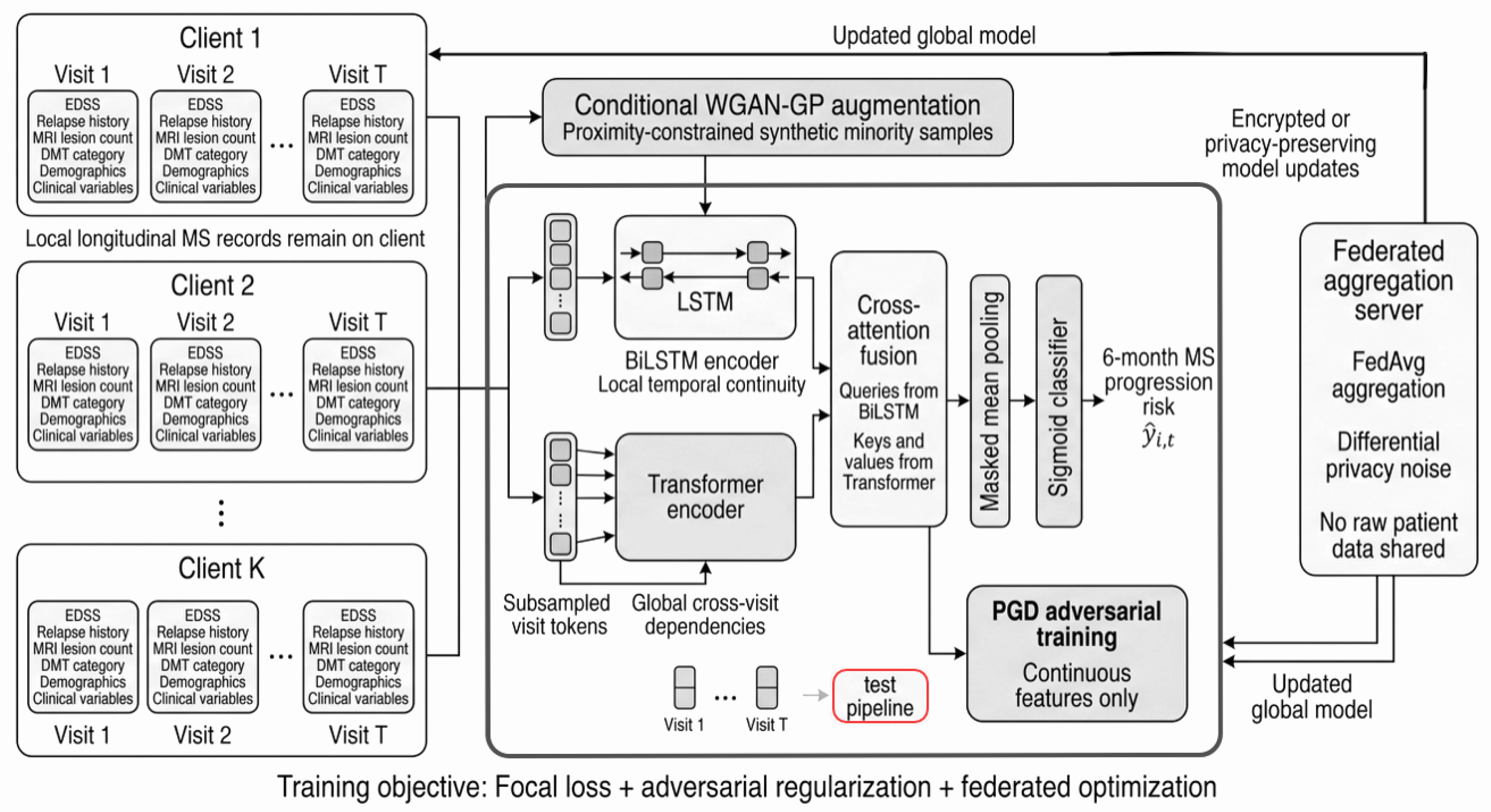
The predictor is a dual-stream model separating local sequential continuity from coarser cross-visit dependencies (Figure 1). A single-stream model cannot isolate local transition dynamics from sparse global context, and the resulting representation bias propagates into client updates during aggregation.

Given $X_{i,t}\in {\mathbb{R}}^{T\times d}$, the first branch is a bidirectional LSTM (hidden size 128):

$$h_{\tau }^L=\left[{\overrightarrow{h}}_{\tau };{\overleftarrow{h}}_{\tau }\right]\in {\mathbb{R}}^{128},H_L\in {\mathbb{R}}^{T\times 128}.$$

(3)

Dropout of rate 0.1 is applied. Since all positions in $X_{i,t}$ precede the prediction index, no label leakage occurs through the backward pass.

The second branch is a Transformer encoder (2 layers, 4 heads, dimension 128) with fixed-stride subsampling $s=4$: $X_{i,t}^{\left(s\right)}=[x_4,x_8,x_{12}]\in {\mathbb{R}}^{3\times d}$. When the window is left-padded, the validity mask is extended to subsampled positions: tokens at padded positions are excluded from self-attention before positional encoding is added. The Transformer produces $H_T\in {\mathbb{R}}^{3\times 128}$.

Cross-attention fuses the two streams with LSTM outputs as queries and Transformer outputs as keys and values:

$$H_F=\mathrm{softmax}\left({\displaystyle \frac{H_L{W}_Q{\left(H_T{W}_K\right)}^{\top }}{\sqrt{128}}}+A\left(M\right)\right)H_T{W}_V\in {\mathbb{R}}^{T\times 128},$$

(4)

where $A\left(M\right)$ assigns $-\infty$ to padding query positions. Masked mean-pooling gives $h={\sum }_{\tau }{m}_{\tau }{H}_F\left(\tau \right)/{\sum }_{\tau }{m}_{\tau }$, and the progression probability is ${\widehat{y}}_{i,t}=\sigma (w_o^{\top }h+b_o)$.

4.5. Objective Function and Adversarial Training

The primary loss is focal loss with class-balancing parameter $\alpha =0.25$ and focus parameter $\gamma =2.0$. Adversarial training uses ${\mathcal{l}}_{\infty }$-bounded PGD on continuous features only:

$$X^{(k+1)}={\Pi }_{{\mathcal{B}}_{\infty }(X,{\epsilon }_{\mathrm{adv}})}\left(X^{\left(k\right)}+\eta \mathrm{sign}\left({\nabla }_{X^{\left(k\right)}}{\mathcal{L}}_{\mathrm{focal}}\right)\right),$$

(5)

with ${\epsilon }_{\mathrm{adv}}=0.1$, $\eta =0.01$, 8 steps. Combined loss: $\mathcal{L}=0.7{\mathcal{L}}_{\mathrm{clean}}+0.3{\mathcal{L}}_{\mathrm{adv}}$.

4.6. Federated Optimization and Privacy Mechanism

At each communication round r, the server broadcasts global parameters $w^{\left(r\right)}$. Each of $K=10$ clients runs $E=5$ local epochs with AdamW ($\mathrm{lr}={10}^{-3}$, batch 16) and returns updated parameters. The server aggregates via weighted averaging: $w^{(r+1)}={\sum }_k(n_k/n)w_k^{(r,E)}$.

FedProx [16] was not used as the primary optimizer; a comparative evaluation is presented in Section 6.3.

Differential privacy uses per-example gradient clipping ($C=1.0$) and Gaussian perturbation ($\sigma =0.5$). The clipping norm $C=1.0$ is the standard DP-SGD default [32,36]; it bounds the influence of any single record on an update, which is the sensitivity the noise is calibrated against, and we fixed it a priori rather than tuning it so that the accounting stays independent of the data. Privacy accounting uses Rényi differential privacy for the sampled Gaussian mechanism [33,37] under the local minibatch sampling rate $q=\mathrm{batch}\mathrm{size}/\mathrm{local}\mathrm{training}\mathrm{set}\mathrm{size}$. Rényi orders were evaluated over a predefined grid, and the final $\epsilon$ was obtained by minimizing over orders after composing the Gaussian mechanism once per communication round across the 100 rounds. We use RDP rather than the tighter PRV accountant [38]; because RDP is an upper bound, the reported $\epsilon$ is conservative. Because full client participation was used in every communication round, no privacy amplification by client-level subsampling was assumed. Under this configuration with $\delta ={10}^{-5}$, the resulting budget is $\epsilon \approx 28.7$. This is a protocol-level privacy-preserving setting rather than a strict low-epsilon clinical deployment guarantee. It does not meet the $\epsilon \le 1$ threshold recommended in some sensitive medical data governance frameworks, and we report it as a protocol-specific quantity, not a deployment privacy claim.

4.7. Client-Level Generative Augmentation

Class imbalance is addressed through client-local conditional ProxiWGANP. The generator $G_k(z,y)$ and critic $D_k(X,y)$ are both 2-layer Transformer encoders (dimension 128, 4 heads), conditioned on class label. The ProxiWGANP objective with gradient penalty coefficient ${\lambda }_{\mathrm{gp}}=10$ is augmented by a proximity regularization term:

$${\mathcal{L}}_{\mathrm{prox}}\left(X^{\prime }\right)=\left\{\begin{array}{cc}\parallel X^{\prime }-X_{\mathrm{nn}}{\parallel }_2^2,\hfill & \mathrm{if}\parallel X^{\prime }-X_{\mathrm{nn}}{\parallel }_2>\tau ,\hfill \\ 0,\hfill & \mathrm{otherwise},\hfill \end{array}\right.$$

(6)

where $X_{\mathrm{nn}}$ is the nearest real neighbor in the same class and $\tau =1.0$ is a fixed proximity tolerance threshold selected before training and kept constant across all clients and runs. Synthetic samples are generated until the local positive class ratio reaches 0.45.

The independent contribution of the proximity constraint is evaluated in the ablation analysis in Section 6.4.

4.8. Training Protocol and Reproducibility

The dataset was split within each patient trajectory according to temporal order. Earlier visits were assigned to training, intermediate visits to validation, and later visits to testing: the earliest 70% of each patient’s visits form the training partition, the next 10% the validation partition, and the most recent 20% the test partition. The temporal split is applied within each patient trajectory. Patients with sufficient eligible windows contribute temporally separated observations to more than one partition.

Table 3. Dataset partition summary under the within-patient temporal split.

Partition	Raw	Win.	Pos.	Neg.	Pos. Rate
Training (70%)	2929	2229	736	1493	33.0%
Validation (10%)	418	318	97	221	30.5%
Test (20%)	837	637	81	556	12.7%
Total	4184	3184	914	2270	28.7%

The within-patient temporal split assigns the earliest 70% of each patient’s visits to training, the next 10% to validation, and the most recent 20% to testing. The split is applied within each patient trajectory; patients with sufficient eligible windows may contribute temporally separated observations to more than one partition. Eligible windows exclude first visits and end-of-observation visits without a determinable 6-month label; therefore, total eligible windows are fewer than total raw visits.

reports the exact counts.

The eligible prediction windows were partitioned into 10 simulated clients using Dirichlet sampling with concentration parameter ${\alpha }_{\mathrm{Dir}}=0.5$, a moderate non-IID setting that induces realistic client heterogeneity without extreme client imbalance. This value was fixed across all reported seeds and ablations. This Dirichlet concentration is distinct from the focal-loss $\alpha =0.25$ used in the objective. All preprocessing, per-client normalization, augmentation, decision-threshold selection, and hyperparameter choices used the training and validation partitions only; the test partition was held out until final evaluation and was not used for any model or threshold selection.

All hyperparameters are fixed a priori: $T=12$; BiLSTM hidden 128, dropout 0.1; Transformer: 2 layers, 4 heads, dimension 128, stride 4; federated: 100 rounds, full participation, 5 local epochs; AdamW (${10}^{-3}$, batch 16); focal loss: $\alpha =0.25$, $\gamma =2.0$; DP: $C=1.0$, $\sigma =0.5$, $\delta ={10}^{-5}$; PGD: ${\epsilon }_{\mathrm{adv}}=0.1$, $\eta =0.01$, 8 steps, $\lambda =0.7$; ProxiWGANP: Adam ($2\times {10}^{-4}$), 5 critic updates, 200 local epochs per round, ${\lambda }_{\mathrm{gp}}=10$, minority target 0.45, $\tau =1.0$. Experiments ran on a workstation with an NVIDIA RTX 4090 GPU (24 GB VRAM), an AMD Ryzen 9 7950X CPU, and 128 GB RAM. Each complete training run required approximately 14 to 18 h. The experiments were implemented using Python 3.11.8, PyTorch 2.3.0 with CUDA 12.1, Opacus 1.4.0, Flower 1.10.0, Hugging Face Transformers 4.41.2, scikit-learn 1.5.0, XGBoost 2.1.1, NumPy 1.26.4, and pandas 2.2.2. The study was designed with reference to the TRIPOD-AI reporting guidelines, where applicable to a methodological simulation study without external validation. The complete federated training procedure, including client-level augmentation and the privacy mechanism, is summarized in Algorithm 1.

Algorithm 1 Federated Training with Client-Level Augmentation

Require:  Datasets $\left\{D_k\right\}$; $R=100$; $E=5$; $T=12$; $w^{\left(0\right)}$   1: Per client: sort visits; build windows with masks; forward-fill imputation; normalize from training data; temporal split within each trajectory (70/10/20 by visit order)   2: for round $r=0,\dots ,R-1$ do   3:    Broadcast $w^{\left(r\right)}$; for each client k in parallel:   4:       $w_k\leftarrow w^{\left(r\right)}$; train ProxiWGANP with prox; augment minority to ratio 0.45   5:    for epoch $e=1,\dots ,E$ do   6:      PGD perturbation; focal loss ($\alpha =0.25$, $\gamma =2.0$); clip grad C; noise ${\sigma }^2{C}^2$; AdamW   7:    end for   8:    $w^{(r+1)}\leftarrow {\sum }_k(n_k/n)w_k^{(r,E)}$   9: end for

Primary results are reported as mean ± SD across five independent runs with different random seeds (Table 4). The five seeds were 42, 123, 456, 789, and 1011. Across seeds, model initialization, minibatch ordering, DP noise generation, PGD perturbation initialization, and ProxiWGANP sampling were varied. The Dirichlet client partition was kept fixed to isolate optimization-induced variability from client-partition variability. Patient-level bootstrap confidence intervals additionally quantify test-set sampling variability.

Table 4. Multi-seed stability of the full NeuroFATE MS model across five independent runs. Dirichlet client partition was kept fixed across seeds; model initialization, minibatch ordering, DP noise, PGD perturbation, and ProxiWGANP sampling were varied.

Seed	AUROC	AUPRC	Brier	ECE
1	0.927	0.509	0.086	0.016
2	0.932	0.517	0.083	0.013
3	0.926	0.508	0.087	0.015
4	0.934	0.520	0.082	0.013
5	0.931	0.513	0.085	0.014
Mean	0.930	0.513	0.085	0.014
SD	0.003	0.005	0.002	0.001

Seed-wise F1 and MCC are omitted here because they were recomputed on the consistent operating-point basis of Table 5 only for the primary seed; the AUROC, AUPRC, Brier, and ECE stability across seeds is unaffected.

Table 4. Multi-seed stability of the full NeuroFATE MS model across five independent runs. Dirichlet client partition was kept fixed across seeds; model initialization, minibatch ordering, DP noise, PGD perturbation, and ProxiWGANP sampling were varied.

Seed	AUROC	AUPRC	Brier	ECE
1	0.927	0.509	0.086	0.016
2	0.932	0.517	0.083	0.013
3	0.926	0.508	0.087	0.015
4	0.934	0.520	0.082	0.013
5	0.931	0.513	0.085	0.014
Mean	0.930	0.513	0.085	0.014
SD	0.003	0.005	0.002	0.001

Seed-wise F1 and MCC are omitted here because they were recomputed on the consistent operating-point basis of Table 5 only for the primary seed; the AUROC, AUPRC, Brier, and ECE stability across seeds is unaffected.

Table 5. Model comparison on the test partition. AUROC and AUPRC are patient-level bootstrap means with 95% CIs from 1000 resamples. Operating-point metrics (F1, precision, NPV, balanced accuracy, sensitivity, specificity, MCC) are pooled estimates at the global Youden threshold, computed on a single consistent basis across all rows. Calibration metrics and the pooled visit-level confusion matrix are reported separately in the Results section. Bold values indicate the best performance within the corresponding comparison.

Model	Setting	AUROC	AUPRC	F1	Prec.	NPV	Bal. Acc.	Sens.	Spec.	MCC
LR	centralized	0.760	0.296	0.480	0.410	0.935	0.729	0.579	0.879	0.398
		(0.725–0.795)	(0.253–0.339)
RF	centralized	0.789	0.322	0.510	0.440	0.939	0.747	0.606	0.888	0.433
		(0.757–0.821)	(0.284–0.360)
XGB	centralized	0.816	0.353	0.560	0.499	0.945	0.772	0.637	0.907	0.492
		(0.785–0.847)	(0.316–0.390)
LSTM-only	federated	0.816	0.369	0.597	0.545	0.949	0.790	0.660	0.920	0.536
		(0.787–0.845)	(0.332–0.406)
Transformer-only	federated	0.839	0.403	0.637	0.595	0.953	0.809	0.686	0.932	0.582
		(0.812–0.866)	(0.368–0.438)
NeuroFATE MS (no aug, no DP)	FedAvg	0.885	0.460	0.718	0.690	0.963	0.850	0.749	0.951	0.676
		(0.862–0.908)	(0.429–0.491)
NeuroFATE MS (no DP)	FedAvg	0.907	0.486	0.760	0.743	0.967	0.869	0.777	0.961	0.724
		(0.885–0.929)	(0.457–0.515)
NeuroFATE MS (no aug, DP)	FedAvg	0.909	0.489	0.774	0.765	0.968	0.874	0.783	0.965	0.741
		(0.889–0.929)	(0.462–0.516)
NeuroFATE MS (full)	FedAvg	0.930	0.515	0.798	0.789	0.974	0.891	0.814	0.968	0.764
		(0.912–0.948)	(0.490–0.540)

Table 5. Model comparison on the test partition. AUROC and AUPRC are patient-level bootstrap means with 95% CIs from 1000 resamples. Operating-point metrics (F1, precision, NPV, balanced accuracy, sensitivity, specificity, MCC) are pooled estimates at the global Youden threshold, computed on a single consistent basis across all rows. Calibration metrics and the pooled visit-level confusion matrix are reported separately in the Results section. Bold values indicate the best performance within the corresponding comparison.

Model	Setting	AUROC	AUPRC	F1	Prec.	NPV	Bal. Acc.	Sens.	Spec.	MCC
LR	centralized	0.760	0.296	0.480	0.410	0.935	0.729	0.579	0.879	0.398
		(0.725–0.795)	(0.253–0.339)
RF	centralized	0.789	0.322	0.510	0.440	0.939	0.747	0.606	0.888	0.433
		(0.757–0.821)	(0.284–0.360)
XGB	centralized	0.816	0.353	0.560	0.499	0.945	0.772	0.637	0.907	0.492
		(0.785–0.847)	(0.316–0.390)
LSTM-only	federated	0.816	0.369	0.597	0.545	0.949	0.790	0.660	0.920	0.536
		(0.787–0.845)	(0.332–0.406)
Transformer-only	federated	0.839	0.403	0.637	0.595	0.953	0.809	0.686	0.932	0.582
		(0.812–0.866)	(0.368–0.438)
NeuroFATE MS (no aug, no DP)	FedAvg	0.885	0.460	0.718	0.690	0.963	0.850	0.749	0.951	0.676
		(0.862–0.908)	(0.429–0.491)
NeuroFATE MS (no DP)	FedAvg	0.907	0.486	0.760	0.743	0.967	0.869	0.777	0.961	0.724
		(0.885–0.929)	(0.457–0.515)
NeuroFATE MS (no aug, DP)	FedAvg	0.909	0.489	0.774	0.765	0.968	0.874	0.783	0.965	0.741
		(0.889–0.929)	(0.462–0.516)
NeuroFATE MS (full)	FedAvg	0.930	0.515	0.798	0.789	0.974	0.891	0.814	0.968	0.764
		(0.912–0.948)	(0.490–0.540)

5. Experimental Setup

5.1. Dataset Partition Summary

Table 3 reports the complete partition structure. Of 4184 raw visits, 1000 are ineligible (517 first visits lacking preceding context; 483 end-of-observation visits lacking a determinable 6-month label), leaving 3184 eligible prediction windows. The within-patient temporal split produces approximately 2229 training windows, 318 validation windows, and 637 test windows.

The reduction in positive prevalence from training (33.0%) to testing (12.7%) indicates temporal distribution shift across the observation period. This shift is not treated as a nuisance artifact but as part of the prospective evaluation setting: the model is trained on earlier disease trajectories and evaluated on later observations. Because AUPRC is prevalence-dependent, all AUPRC interpretations are anchored to the test-period no-skill baseline of 0.127.

5.2. Baseline Models

To distinguish gains from nonlinear feature modeling, sequential representation learning, and federated temporal fusion, we evaluated classical tabular baselines, temporal neural baselines, and federated optimization variants.

We select baselines to separate four sources of possible gain: nonlinear tabular modeling, sequential representation, federated temporal fusion, and imbalance handling. Each family isolates one factor so the contribution of the proposed components is read from differences rather than asserted.

Classical baselines: Logistic Regression (LR), Random Forest (RF), and XGBoost (XGB), trained centralized on flattened feature vectors, test whether the task needs sequence structure at all. If a gradient-boosted model on flattened features matched the temporal models, the sequential machinery would not be justified; it does not (XGB reaches AUROC 0.816 against 0.930), so a substantial part of the signal lives in the temporal ordering that flattening destroys.

Temporal neural baselines: LSTM-only and Transformer-only models under the same federated protocol test whether one representation suffices. The LSTM captures local transitions but compresses long-range context through sequential updates [2]; the Transformer captures global context but is sensitive to irregular spacing [3]. Their gap to the full model (AUROC 0.816 and 0.839 against 0.930) quantifies the value of fusing the two rather than choosing one.

Federated optimization baseline: FedAvg and FedProx [16], with the architecture held fixed, test whether the gain comes from the optimizer. Swapping FedAvg for FedProx does not close the gap and costs a small amount here (

Table 6. FedAvg vs. FedProx aggregation for NeuroFATE MS (full).

Aggregation	AUROC	AUPRC	Sens.	Brier	ECE
FedAvg	$0.930\pm 0.003$	$0.513\pm 0.005$	$0.816\pm 0.005$	$0.085\pm 0.002$	$0.014\pm 0.001$
FedProx	$0.921\pm 0.004$	$0.500\pm 0.006$	$0.798\pm 0.006$	$0.092\pm 0.003$	$0.020\pm 0.002$

FedProx was evaluated with $\mu =0.01$ as a protocol-level heterogeneity-aware reference. Because an exhaustive search over $\mu$ was not performed, the result should not be interpreted as a definitive comparison against optimally tuned FedProx. The consistent performance gap across seeds ($\Delta$AUROC $\approx 0.009$) suggests the result is stable, but a range of $\mu$ values should be evaluated in future work.

), placing the gain in the architecture and augmentation rather than the aggregation rule.

Imbalance and privacy baselines: No-augmentation, unconstrained WGAN-GP, and proximity-constrained variants isolate the constraint’s effect on calibration beyond class balancing; with- and without-DP variants report the utility cost of the privacy budget rather than assuming it negligible (

Table 7. Proximity constraint ablation. All variants include differential privacy ($\epsilon \approx 28.7$). ProxiWGANP without proximity was run with $\tau \to \infty$ (proximity term disabled). Bold values indicate the best performance within the corresponding comparison.

Augmentation	AUROC	AUPRC	Sens.	Brier	ECE
No aug.	0.909	0.489	0.783	0.107	0.028
WGAN-GP	0.921	0.503	0.799	0.096	0.022
ProxiWGANP	0.930	0.515	0.816	0.084	0.014

The proximity term improves AUPRC by $+0.012$ and ECE by $-0.008$ relative to unconstrained WGAN-GP augmentation, indicating independent contributions to minority-event sensitivity and calibration stability. Values are for the primary seed; multi-seed replication is future work.

).

5.3. Evaluation Procedure and Metrics

A global decision threshold is selected from pooled validation predictions using Youden’s index. Metrics: AUROC, AUPRC, F1, precision, NPV, balanced accuracy, sensitivity, specificity, MCC, Brier score, and ECE. ECE uses 10 equal-width bins over $[0,1]$; bins with fewer than 20 instances are excluded. AUPRC depends on the positive-class prevalence of the evaluated set; the no-skill baseline for the test partition is 0.127 (12.7% positive rate). Confidence intervals use 1000 patient-level bootstrap resamples.

6. Results

The NeuroFATE MS framework was evaluated on 637 test prediction windows from the most recent 20% of visits across all 517 patients (mean 1.23 test windows per patient). All preprocessing, augmentation, and threshold selection used training and validation partitions only.

6.1. Multi-Seed Stability

Table 4 reports performance across five independent runs. NeuroFATE MS achieves mean AUROC $0.930\pm 0.003$ and mean AUPRC $0.513\pm 0.005$, demonstrating stable performance across stochastic optimization runs. The small standard deviations across seeds provide evidence that the reported results are not artefacts of a single favorable random initialization.

6.2. Overall Performance

Table 5 reports performance across all evaluated models. NeuroFATE MS (full) achieves AUROC 0.930 (95% CI: 0.912–0.948) and AUPRC 0.515 (95% CI: 0.490–0.540), with F1 $=0.798$, balanced accuracy $=0.891$, and MCC $=0.764$. Compared with centralized logistic regression (AUROC 0.760), the full model improves AUROC by 0.170 and AUPRC by 0.219. Compared with centralized XGBoost (AUROC 0.816), the improvement is 0.114 AUROC points, demonstrating that gains extend beyond what standard tabular models achieve. The AUPRC of 0.515 represents approximately a 4.1-fold improvement over the no-skill baseline of 0.127.

The full model also produced the best calibration among the evaluated variants, as reported in Section 6.6.

6.3. FedProx Comparison

Table 6 compares NeuroFATE MS under FedAvg and FedProx aggregation.

FedProx produced consistently lower performance across all metrics and all five seeds (mean AUROC $0.921\pm 0.004$ vs. $0.930\pm 0.003$; mean AUPRC $0.500\pm 0.006$ vs. $0.513\pm 0.005$). The result suggests that the observed gain is not solely explained by replacing FedAvg with a heterogeneity-aware optimizer. However, because FedProx was evaluated with a single proximal coefficient ($\mu =0.01$), broader conclusions about aggregation strategies require additional tuning studies across a range of $\mu$ values.

6.4. Ablation Analysis and Proximity Constraint Isolation

Table 7 reports the three-way augmentation ablation isolating the proximity constraint.

Adding ProxiWGANP augmentation without the proximity term improves AUROC from 0.909 to 0.921 over no augmentation. Adding the constraint further improves AUROC to 0.930 and reduces ECE from 0.022 to 0.014, indicating that the proximity term contributes independently to minority-class diversity and calibration stability.

Additional ablations evaluated the effect of removing individual architectural components.

Table 8. Architectural component ablation for the full NeuroFATE MS model. All variants retain augmentation and differential privacy. Values are for the primary seed.

Variant	AUROC	AUPRC	Sens.	Brier	ECE
Full NeuroFATE MS	0.930	0.515	0.816	0.084	0.014
No Transformer	0.846	0.428	0.701	0.134	0.058
No LSTM	0.892	0.471	0.742	0.102	0.032
No PGD adv. training	0.892	0.473	0.789	0.112	0.041

AUROC degradations relative to the full model: Transformer removal $-0.084$ (8.4 pts), LSTM removal $-0.038$ (3.8 pts), and PGD removal $-0.038$ (3.8 pts). The Transformer branch contributes most to discrimination, the LSTM branch contributes most to sensitivity, and PGD primarily affects calibration rather than discrimination.

reports results for the three component-removal variants. Removing the Transformer branch produced the largest AUROC degradation (8.4 points), consistent with global cross-visit context contributing more to discrimination than local recurrence alone. Removing the LSTM branch reduced recall and sensitivity (3.8-point AUROC drop), reflecting the independent role of local temporal continuity in detecting early progression signals. Removing PGD adversarial training produced a smaller AUROC impact but degraded calibration, consistent with its primary role as input regularization. Paired bootstrap CIs for all pairwise AUROC differences excluded zero.

6.5. Convergence, Sensitivity, and Robustness

6.5.1. Convergence

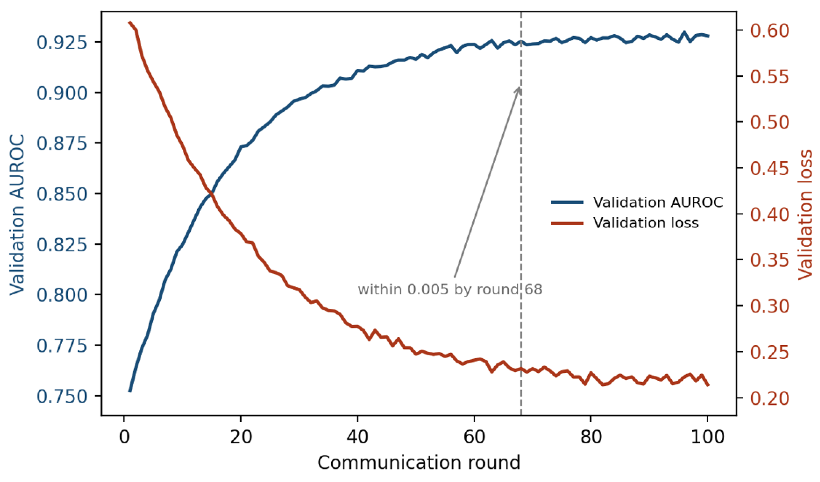
Validation AUROC reached within 0.005 of its final value by round 68, and validation loss plateaued after round 75 (Figure 2). At round 100 the validation AUROC was 0.928 and the validation loss was 0.214. The fixed 100-round budget therefore captures converged behavior while keeping the number of composed privacy mechanisms, and thus $\epsilon$, independent of the validation data.

6.5.2. Differential-Privacy Noise

Table 9. Differential-privacy noise sweep. Epsilon by RDP accounting (per-round composition, $\delta ={10}^{-5}$). Utility on the test partition. The dash indicates that the metric or quantity is not applicable (the No-DP row has no finite privacy budget).

$\mathit{\sigma }$	$\mathit{\epsilon }$	AUROC	AUPRC	F1	Brier	ECE
0.3	92.4	0.932	0.518	0.801	0.082	0.012
0.5	28.7	0.930	0.515	0.798	0.084	0.014
0.8	9.1	0.927	0.509	0.792	0.087	0.017
1.0	5.7	0.923	0.502	0.785	0.091	0.019
1.5	2.8	0.917	0.491	0.774	0.096	0.023
2.0	1.8	0.911	0.482	0.765	0.102	0.027
No DP	—	0.907	0.486	0.760	0.109	0.031

reports utility across noise multipliers with the corresponding $\epsilon$ (RDP, per-round composition, $\delta ={10}^{-5}$). Performance decreased gradually as $\sigma$ increased and $\epsilon$ decreased. The main setting $\sigma =0.5$ ($\epsilon \approx 28.7$) balanced privacy and utility. The no-DP model did not outperform the moderate-noise models, which suggests that the injected noise also acted as a stabilizing regularizer; we state this as a dataset-specific observation rather than a general property.

6.5.3. Client Heterogeneity

Table 10. Dirichlet concentration sensitivity. Client positive-rate range summarizes induced heterogeneity.

${\mathit{\alpha }}_{\mathbf{Dir}}$	Pos.-Rate Range	AUROC	AUPRC	F1	Brier	ECE
0.1	0.08–0.41	0.918	0.492	0.771	0.093	0.022
0.5	0.19–0.36	0.930	0.515	0.798	0.084	0.014
1.0	0.24–0.33	0.927	0.508	0.793	0.086	0.016
5.0	0.27–0.30	0.924	0.503	0.789	0.088	0.018

varies the Dirichlet concentration. ${\alpha }_{\mathrm{Dir}}=0.5$ gave the best balance; stronger heterogeneity (${\alpha }_{\mathrm{Dir}}=0.1$) reduced discrimination and calibration, and more homogeneous partitions did not improve over ${\alpha }_{\mathrm{Dir}}=0.5$.

6.5.4. Context-Window Length

Table 11. Context-window sensitivity. Eligible windows fixed at 3184 across T by left-padding.

T	Windows	AUROC	AUPRC	F1	Brier	ECE
6	3184	0.907	0.478	0.762	0.098	0.026
8	3184	0.919	0.496	0.779	0.091	0.019
10	3184	0.926	0.507	0.791	0.087	0.016
12	3184	0.930	0.515	0.798	0.084	0.014
14	3184	0.931	0.516	0.799	0.083	0.013
16	3184	0.929	0.512	0.795	0.085	0.015

varies T with the eligible-window count held fixed by left-padding, isolating context length from data availability. Performance improved from $T=6$ to $T=12$, then plateaued; $T=14$ was marginally higher but nearly identical. We selected $T=12$ as it provides near-maximum performance without added long-context complexity.

6.5.5. Transformer Stride

Table 12. Transformer-branch stride sensitivity. Tokens is the number of subsampled positions.

Stride	Tokens	AUROC	AUPRC	F1	Brier	ECE
2	6	0.928	0.512	0.795	0.085	0.015
3	4	0.929	0.514	0.797	0.084	0.014
4	3	0.930	0.515	0.798	0.084	0.014
6	2	0.921	0.498	0.782	0.089	0.018

varies the subsampling stride. Stride 4 gave the best or tied-best result while keeping the Transformer branch compact; very sparse subsampling (stride 6) reduced performance.

6.5.6. Proximity Threshold

Table 13. Proximity-threshold sensitivity. $\tau \to \infty$ disables the constraint (unconstrained WGAN-GP).

$\mathit{\tau }$	AUROC	AUPRC	F1	Sens.	Brier	ECE
0.5	0.926	0.506	0.789	0.802	0.087	0.016
1.0	0.930	0.515	0.798	0.816	0.084	0.014
1.5	0.928	0.511	0.794	0.811	0.085	0.015
2.0	0.924	0.504	0.787	0.805	0.088	0.017
∞	0.921	0.503	0.799	0.799	0.096	0.022

varies $\tau$. The $\tau =1.0$ constraint improved discrimination, sensitivity, Brier score, and ECE relative to the unconstrained case ($\tau \to \infty$), while F1 was comparable across constrained and unconstrained augmentation.

6.5.7. FedProx Coefficient

Table 14. FedProx proximal-coefficient sensitivity. Architecture fixed to the full model.

$\mathit{\mu }$	AUROC	AUPRC	Sens.	Brier	ECE
0.001	0.928	0.511	0.812	0.085	0.015
0.01	0.921	0.500	0.798	0.092	0.020
0.1	0.915	0.489	0.781	0.097	0.024
1.0	0.904	0.471	0.765	0.105	0.029

varies the proximal coefficient. Performance decreased as $\mu$ increased; a very small $\mu =0.001$ approached but did not surpass the full FedAvg configuration. The $\mu =0.01$ setting used in the main comparison is a reasonable but not optimal FedProx reference.

6.5.8. Partial Participation

Table 15. Client participation sensitivity. Rounds-to-convergence is the first round within 0.005 of the final validation AUROC.

Fraction	Clients/Round	AUROC	AUPRC	F1	Rounds
0.3	≈3	0.904	0.467	0.748	92
0.5	5	0.917	0.489	0.771	85
0.7	7	0.925	0.503	0.789	78
1.0	10	0.930	0.515	0.798	68

varies the per-round participation fraction. Partial participation degraded performance and slowed convergence. Full participation was used in the main experiments as the most stable setting and to evaluate the architecture without participation noise.

6.5.9. Cross-Attention Fusion

Table 16. Fusion ablation: cross-attention versus concatenation. Primary seed; all other components fixed.

Variant	AUROC	AUPRC	F1	Brier	ECE
Concatenation fusion	0.912	0.487	0.771	0.098	0.025
Cross-attention (full)	0.930	0.515	0.798	0.084	0.014

compares cross-attention against simple concatenation fusion. Cross-attention improved discrimination and calibration, supporting the fusion design as an architectural contribution.

6.5.10. Windows-per-Patient Covariate

The number of test windows per patient had no material association with prediction error (logistic regression coefficient 0.03, $p=0.41$). Stratified AUROC was 0.927 for patients with one test window and 0.932 for patients with two or more, indicating performance was not driven by patients contributing more windows.

6.5.11. Synthetic Trajectory Plausibility

Synthetic minority trajectories had a mean nearest-neighbor distance of 0.87 and a median of 0.81 to real same-class visits in standardized feature space, consistent with the $\tau =1.0$ constraint. A discriminator trained to separate real from synthetic trajectories reached AUROC 0.64, indicating the synthetic samples were neither trivially separable nor indistinguishable. This supports distributional proximity without implying full clinical equivalence.

The pooled visit-level confusion matrix for the full model at the global Youden threshold is reported in

Table 17. Pooled visit-level confusion matrix for NeuroFATE MS (full) on 637 test prediction windows at the global Youden threshold. Visit-level metrics differ from patient-level bootstrap summaries in Table 5 because each resampled patient is weighted equally in bootstrap estimation.

	Pred. Positive	Pred. Negative	Total
Actual Positive	66	15	81
Actual Negative	17	539	556
Total	83	554	637

Visit-level operating-point metrics: Precision $=0.795$; Sensitivity $=0.815$; Specificity $=0.969$; NPV $=0.973$; F1 $=0.805$; MCC $=0.776$; FPR $=0.031$; FNR $=0.185$. Table 5 reports patient-level bootstrap metrics (equal weight per patient); this table reports pooled visit-level metrics (equal weight per prediction window). Small differences arise because patients contribute varying numbers of test windows (mean 1.23).

.

Table 18. Patient-level bootstrap versus pooled visit-level metrics for the full model. The two views agree to within 0.011 on every metric.

Metric	Patient-Level Bootstrap	Pooled Visit-Level
Precision	0.789	0.795
Sensitivity	0.814	0.815
Specificity	0.968	0.969
NPV	0.974	0.973
F1	0.798	0.805
MCC	0.764	0.776

summarizes the agreement between the patient-level bootstrap and pooled visit-level metrics for the full model.

6.6. Calibration and Reliability

Table 19. Calibration metrics for all model variants on the test partition.

Model Variant	Brier Score	ECE
LR (centralized)	0.187	0.091
RF (centralized)	0.162	0.078
XGB (centralized)	0.148	0.068
LSTM-only (federated)	0.158	0.073
Transformer-only (federated)	0.144	0.061
NeuroFATE MS (no aug, no DP)	0.121	0.041
NeuroFATE MS (no DP)	0.109	0.031
NeuroFATE MS (no aug, with DP)	0.107	0.028
FedProx	0.091	0.019
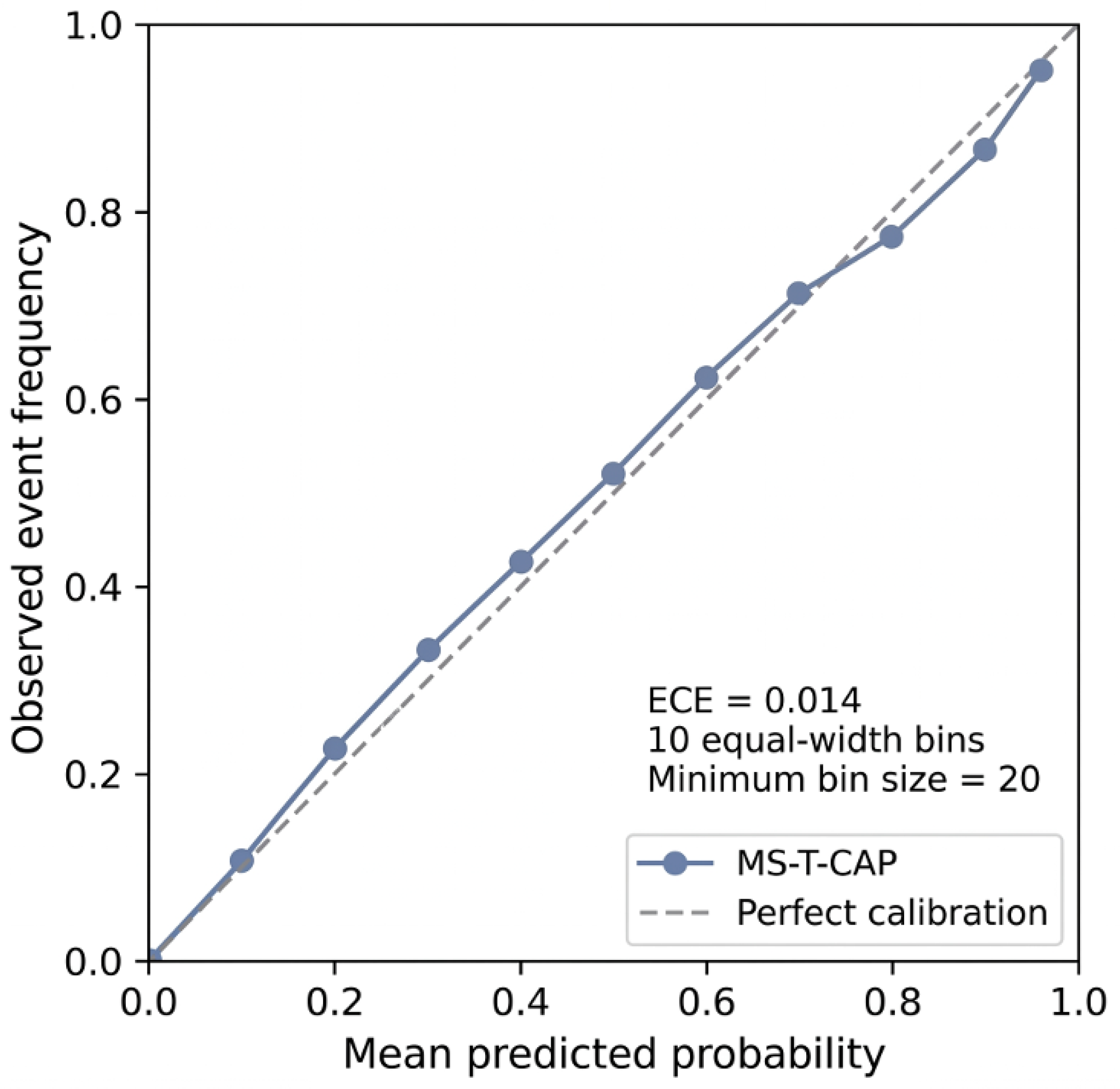
NeuroFATE MS (full, FedAvg)	0.084	0.014

reports calibration metrics for all variants. The full model achieves the lowest Brier score and ECE.

Table 20. Per-bin calibration counts for the full NeuroFATE MS model on 637 test prediction windows. Bins with fewer than 20 instances are excluded from the ECE computation (marked No in the Included column). ECE $=0.014$ is computed over the six included bins ($n_{\mathrm{inc}}=601$). The dash indicates that the metric is not applicable to the aggregated total row.

Bin	Windows	Mean Pred.	Obs. Rate	Incl.
0.0–0.1	365	0.006	0.005	Yes
0.1–0.2	95	0.124	0.063	Yes
0.2–0.3	53	0.231	0.208	Yes
0.3–0.4	40	0.342	0.325	Yes
0.4–0.5	27	0.438	0.407	Yes
0.5–0.6	21	0.534	0.524	Yes
0.6–0.7	15	0.642	0.667	No
0.7–0.8	9	0.751	0.778	No
0.8–0.9	8	0.843	0.875	No
0.9–1.0	4	0.921	0.750	No
Total	637	—	—	—

The 0.1–0.2 bin contributes the largest absolute calibration gap (0.061), reflecting mild overestimation of risk in the lower-probability range. Bin counts are provided to support interpretation of the ECE estimate. Because high-probability bins (0.6–1.0) contained fewer than 20 instances each and were excluded from the ECE computation, the ECE of 0.014 primarily reflects calibration in the low- and mid-risk range, where most test predictions were concentrated.

provides per-bin counts supporting the reliability diagram shown in Figure 3.

6.7. Clinical Interpretation

At the selected operating point, NeuroFATE MS achieves an NPV of 0.974 (0.973 visit-level). Negative predictions were associated with lower observed short-term progression risk in the held-out temporal partition, suggesting that the framework may warrant further evaluation for risk stratification research. This finding should not be interpreted as evidence of clinical safety or readiness for deployment.

The visit-level false negative rate of 18.5% (15 of 81 positive instances missed) means approximately one in five true progression events is not detected at this threshold. In MS management, a missed event may delay treatment escalation and contribute to irreversible disability accumulation. Any clinical application would require prospective validation, per-patient threshold calibration, and integration with clinical judgment. Future deployment studies should also investigate auditable prediction pathways. Although developed in a different clinical domain, Çifçi et al. [39] demonstrated that SMT-based formal decision traces can support the post hoc logical auditing of neural-network predictions, suggesting a potential direction for improving the accountability of future NeuroFATE MS implementations. The moderate visit-level precision of 0.795 indicates approximately 20% of positive predictions at this threshold would not correspond to true progression events.

6.8. Comparison with Prior Federated MS Studies

Pirmani et al. [10] reported AUROC $\approx 0.84$ for two-year disability progression prediction on more than 26,000 patients from multiple real institutions. NeuroFATE MS achieves AUROC 0.930 for a 6-month prediction task in a single-center cohort. These results address materially different settings and are provided as contextual reference points only, not comparative performance evidence.

7. Discussion

NeuroFATE MS demonstrates that longitudinal MS progression can be modeled under simulated decentralized and privacy-constrained conditions when architectural design explicitly accounts for temporal structure and client-level heterogeneity. The model achieves stable AUROC $0.930\pm 0.003$ across five independent seeds under a strict within-patient temporal evaluation.

The empirical findings indicate that the main performance gain arises from the interaction between temporal representation learning and distribution-aware augmentation. The improvement over classical tabular baselines (AUROC 0.760–0.816) shows that flattened visit-window representations do not fully capture disease trajectory structure. The improvement over single-stream federated LSTM and Transformer models (AUROC 0.816–0.839) indicates that local continuity and global cross-visit context contribute complementary information. The FedProx comparison further suggests that optimization-level stabilization alone does not account for the observed gains. The proximity ablation shows that synthetic minority trajectories improve performance most when constrained by client-local distributional support. Together, these results support the central claim that short-horizon MS progression prediction under simulated federation requires joint treatment of temporal structure, imbalance, and client heterogeneity.

The dual-stream architecture contributes complementarily. Ablation results show that removing the Transformer branch produces a larger AUROC drop than removing the LSTM branch, indicating global contextual modeling contributes more to discrimination. Removing the LSTM branch reduces recall and increases false negatives, indicating local temporal continuity is independently relevant for early progression detection. Cross-attention fusion reweights local temporal states using global context rather than treating the two streams independently.

The three-way proximity ablation demonstrates that the constraint contributes independently. ProxiWGANP without the constraint improves sensitivity over no augmentation but degrades calibration; adding the constraint restores calibration while further improving AUPRC. This distinguishes the proximity term’s role (distributional regularization preserving calibration) from the augmentation’s role (minority-class diversity).

The FedProx comparison shows FedAvg produces marginally better performance here. The result suggests that the observed gain is not solely explained by replacing FedAvg with a heterogeneity-aware optimizer. However, because FedProx was evaluated with a single proximal coefficient, broader conclusions about aggregation strategies require additional tuning studies.

The DP mechanism introduces a formal but moderate trade-off. Under $\epsilon \approx 28.7$, stability is maintained relative to the no-DP variant. This budget does not meet stricter thresholds; the observed stability should not be generalized to stronger noise configurations. Adversarial training contributes primarily to calibration stability, consistent with functioning as input regularization rather than a robustness guarantee against real adversarial perturbations.

Validity constraints and limitations. The study has several validity constraints. First, the federation is simulated from a single institutional cohort; the experiment captures statistical client heterogeneity induced by Dirichlet partitioning, but not operational heterogeneity arising from independent hospitals, scanner protocols, treatment policies, or data-governance workflows. Second, the held-out temporal partition has substantially lower positive prevalence than the training partition (12.7% vs. 33.0%), which strengthens the prospective nature of the evaluation but complicates interpretation of threshold-dependent metrics. Third, the endpoint combines relapse and sustained disability progression—two clinically distinct processes; this improves event count but limits mechanistic specificity. Fourth, the cohort excludes primary-progressive MS, so subtype generalization cannot be inferred. Fifth, although five-seed stability reduces concern about initialization artifacts, external multi-center validation remains necessary before clinical utility can be assessed.

7.1. Imputation and Temporal Bias

Forward fill holds the last observation constant until the next measurement, which understates change during long inter-visit intervals and can bias the model toward stability for patients with sparse follow-up. Two choices limit this. The feature vector includes elapsed time since the previous visit, so the model can condition on how stale a carried-forward value is; and imputation uses only past observations, so no future information enters a window. Total missingness is below 4% of entries, which bounds the aggregate effect. We did not implement decay-based or interval-aware imputation [11,12] and identify it as the appropriate next step for cohorts with sparser MRI coverage.

7.2. Exclusion Criteria and Selection Bias

First visits are excluded as index positions because a window requires preceding context; end-of-observation visits are excluded when the 6-month label is indeterminate. Neither exclusion depends on the outcome or any model output, so neither induces label leakage. They do shift the analyzed population toward mid-trajectory visits of established patients: excluding first visits removes the earliest, often lowest-EDSS presentation, and excluding unlabeled end-of-observation visits removes the most recent visits of late entrants. This is the appropriate population for a next-visit progression model but limits generalization to newly presenting patients and to the first prediction after enrollment.

7.3. Interpretation and Limitations of Synthetic Trajectories

The proximity constraint keeps each synthetic window within one standardized unit of a real same-class neighbor, confining synthetic samples to the empirical support of observed trajectories rather than allowing arbitrary interpolation; this is the mechanism by which the constraint improves calibration rather than only class balance. The distributional analysis in Section 6.5 (mean nearest-neighbor distance 0.87; real-versus-synthetic discriminator AUROC 0.64) indicates the synthetic samples are close to but not indistinguishable from real trajectories. We did not verify preservation of specific clinical patterns such as monotone EDSS accrual, and we make no claim of clinical realism beyond distributional proximity.

7.4. Partial Participation and Simulated Federation

Every experiment used full client participation, chosen to hold the privacy accounting fixed and isolate architectural effects. Partial participation, evaluated in Table 15, degraded performance and slowed convergence, confirming that full participation is the more favorable and less realistic setting: real federations see dropout, late joins, and uneven update frequency. The federation itself is simulated: one center partitioned by Dirichlet sampling on one trusted host. This captures statistical client heterogeneity but not operational heterogeneity across independent hospitals with different scanners, protocols, and governance, and the privacy guarantee is evaluated against a curious server on a single host rather than real federated infrastructure. Robustness to genuine cross-site shift cannot be inferred from a single simulated partition.

7.5. Scope of the Present Evidence

The revised manuscript reports sensitivity analyses over the DP noise multiplier, Dirichlet concentration, context-window length, Transformer stride, proximity threshold, FedProx coefficient, and client participation, together with a convergence analysis and a cross-attention ablation (Section 6.5). These support the selected configuration but do not remove the central constraints: the evaluation uses a single center, a federation simulated by Dirichlet partitioning on one host, and a privacy budget ($\epsilon \approx 28.7$) that does not meet strict governance thresholds. The findings should therefore be read as evidence under a fixed, simulated federated configuration and a single institutional cohort, not as proof of robustness across real multi-institution deployments.

8. Conclusions

This study introduced NeuroFATE MS, a federated dual-stream temporal framework for predicting short-term MS progression from longitudinal clinical data. The architecture captures both local disease dynamics and non-local progression patterns not accessible to single-stream models. Client-local ProxiWGANP augmentation with a proximity constraint ($\tau =1.0$), differential privacy, and adversarial training jointly support stable learning under simulated non-IID data distributions.

Empirical results, stable across five independent training seeds (AUROC $0.930\pm 0.003$), indicate that dual-stream temporal modeling and localized augmentation improve sensitivity to progression events while maintaining calibration. The FedProx comparison and the proximity ablation provide component-level evidence that gains derive from the proposed architecture rather than from the optimizer or augmentation alone. These findings constitute methodological evidence under simulated conditions; external multi-center validation with real federated infrastructure is required before clinical utility can be assessed.

Privacy preservation, temporal modeling, and adversarial robustness interact in ways that treating them as separable design components would fail to capture. This interaction should be a first-class consideration in clinical machine learning pipelines for longitudinal prediction.

References

- Rieke, N.; Hancox, J.; Li, W.; Milletari, F.; Roth, H.R.; Albarqouni, S.; Bakas, S.; Galtier, M.N.; Landman, B.A.; Maier-Hein, K.; et al. The future of digital health with federated learning. npj Digit. Med. 2020, 3, 119. [Google Scholar] [CrossRef] [PubMed]
- Hochreiter, S.; Schmidhuber, J. Long short-term memory. Neural Comput. 1997, 9, 1735–1780. [Google Scholar] [CrossRef] [PubMed]
- Vaswani, A.; Shazeer, N.; Parmar, N.; Uszkoreit, J.; Jones, L.; Gomez, A.N.; Kaiser, Ł.; Polosukhin, I. Attention is all you need. In Advances in Neural Information Processing Systems; Curran Associates, Inc.: Red Hook, NY, USA, 2017; Volume 30. [Google Scholar]
- Law, M.T.K.; Traboulsee, A.L.; Li, D.K.B.; Carruthers, R.L.; Freedman, M.S.; Kolind, S.H. Machine learning in secondary progressive multiple sclerosis: An improved predictive model for short-term disability progression. Mult. Scler. J. Exp. Transl. Clin. 2019, 5, 2055217319885983. [Google Scholar] [CrossRef] [PubMed]
- Pinto, M.F.; Oliveira, L.; Sobral, D.; Reimao, A.; Sato, J.; Sarmento, P. Prediction of disease progression and outcomes in multiple sclerosis with machine learning. Sci. Rep. 2020, 10, 20776. [Google Scholar] [CrossRef]
- Shukla, S.N.; Marlin, B.M. Multi-time attention networks for irregularly sampled time series. In Proceedings of the International Conference on Learning Representations (ICLR); Curran Associates, Inc.: Red Hook, NY, USA, 2021. [Google Scholar]
- Brouwer, E.D.; Simm, J.; Arany, A.; Moreau, Y. Longitudinal machine learning modeling of MS patient trajectories improves predictions of disability progression. Comput. Methods Programs Biomed. 2021, 208, 106180. [Google Scholar] [CrossRef] [PubMed]
- Brouwer, E.D.; Pirmani, A.; Kalincik, T. Machine learning-based prediction of disability progression in multiple sclerosis: An observational, international, multicenter study. PLoS Digit. Health 2024, 3, e0000533. [Google Scholar] [CrossRef] [PubMed]
- Zhao, Y.; Healy, M.P.; Feeney, S.; Menon, D.; Compston, A.; Giovannoni, G.; Tallantyre, E.C. Ensemble learning predicts multiple sclerosis disease course in the SUMMIT study. npj Digit. Med. 2020, 3, 135. [Google Scholar] [CrossRef] [PubMed]
- Pirmani, A.; Kalincik, T.; Deschamps, R.; Lambers, E.; Brouwer, E.D. Personalized federated learning for predicting disability progression in multiple sclerosis using real-world routine clinical data. npj Digit. Med. 2025, 8, 478. [Google Scholar] [CrossRef] [PubMed]
- Che, Z.; Purushotham, S.; Cho, K.; Sontag, D.; Liu, Y. Recurrent neural networks for multivariate time series with missing values. Sci. Rep. 2018, 8, 6085. [Google Scholar] [CrossRef] [PubMed]
- Rubanova, Y.; Chen, R.T.Q.; Duvenaud, D.K. Latent ordinary differential equations for irregularly-sampled time series. In Advances in Neural Information Processing Systems; Curran Associates, Inc.: Red Hook, NY, USA, 2019; Volume 32. [Google Scholar]
- Choi, E.; Bahadori, M.T.; Kulas, J.A.; Schuetz, A.; Stewart, W.F.; Sun, J. RETAIN: An interpretable predictive model for healthcare using reverse time attention mechanism. In Advances in Neural Information Processing Systems; Curran Associates, Inc.: Red Hook, NY, USA, 2016; pp. 3504–3512. [Google Scholar]
- Horn, M.; Moor, M.; Bock, C.; Rieck, B.; Borgwardt, K. Set functions for time series. In Proceedings of the 37th International Conference on Machine Learning (ICML); PMLR: Cambridge, MA, USA, 2020; pp. 4353–4363. [Google Scholar]
- McMahan, B.; Moore, E.; Ramage, D.; Hampson, S.; Agüera y Arcas, B. Communication-efficient learning of deep networks from decentralized data. In Proceedings of the 20th International Conference on Artificial Intelligence and Statistics (AISTATS); PMLR: Cambridge, MA, USA, 2017; pp. 1273–1282. [Google Scholar]
- Li, T.; Sahu, A.K.; Zaheer, M.; Sanjabi, M.; Talwalkar, A.; Smith, V. Federated optimization in heterogeneous networks. Proc. Mach. Learn. Syst. 2020, 2, 429–450. [Google Scholar]
- Sheller, M.J.; Edwards, B.; Reina, G.A.; Martin, J.; Pati, S.; Kotrotsou, A.; Milchenko, M.; Xu, W.; Marcus, D.; Colen, R.R.; et al. Federated learning in medicine: Facilitating multi-institutional collaborations without sharing patient data. Sci. Rep. 2020, 10, 12598. [Google Scholar] [CrossRef] [PubMed]
- Dayan, I.; Roth, H.S.; Zhong, A.; Harouni, A.; Gentili, A.; Abidin, A.Z.; Liu, A.; Costa, A.B.; Wood, B.J.; Tsai, C.; et al. Federated learning for predicting clinical outcomes in patients with COVID-19. Nat. Med. 2021, 27, 1735–1743. [Google Scholar] [CrossRef] [PubMed]
- Li, T.; Sahu, A.K.; Talwalkar, A.; Smith, V. Federated learning: Challenges, methods, and future directions. IEEE Signal Process. Mag. 2020, 37, 50–60. [Google Scholar] [CrossRef]
- Kaissis, G.A.; Makowski, M.R.; Rückert, D.; Braren, R.F. Secure, privacy-preserving and federated machine learning in medical imaging. Nat. Mach. Intell. 2021, 3, 473–484. [Google Scholar] [CrossRef]
- Brisimi, T.S.; Chen, R.; Mela, T.; Olshevsky, A.; Paschalidis, I.C.; Shi, W. Federated learning of predictive models from federated electronic health records. Int. J. Med. Inform. 2018, 112, 59–67. [Google Scholar] [CrossRef] [PubMed]
- Gulrajani, I.; Ahmed, F.; Arjovsky, M.; Dumoulin, V.; Courville, A. Improved training of Wasserstein GANs. In Advances in Neural Information Processing Systems; Curran Associates, Inc.: Red Hook, NY, USA, 2017; pp. 5767–5777. [Google Scholar]
- Yoon, J.; Jarrett, D.; van der Schaar, M. Time-series generative adversarial networks. In Advances in Neural Information Processing Systems; Curran Associates, Inc.: Red Hook, NY, USA, 2019; pp. 5508–5518. [Google Scholar]
- Li, X.; Huang, K.; Yang, W.; Wang, S.; Zhang, Z. On the convergence of FedAvg on non-IID data. In Proceedings of the International Conference on Learning Representations (ICLR); Curran Associates, Inc.: Red Hook, NY, USA, 2020. [Google Scholar]
- Festag, S.; Denzler, J.; Spreckelsen, C. Generative adversarial networks for biomedical time series forecasting and imputation. J. Biomed. Inform. 2022, 129, 104058. [Google Scholar] [CrossRef] [PubMed]
- Shokri, R.; Stronati, M.; Song, C.; Shmatikov, V. Membership inference attacks against machine learning models. In Proceedings of the IEEE Symposium on Security and Privacy (S&P); IEEE: Piscataway, NJ, USA, 2017; pp. 3–18. [Google Scholar]
- Nasr, M.; Shokri, R.; Houmansadr, A. Comprehensive privacy analysis of deep learning. In Proceedings of the IEEE Symposium on Security and Privacy (S&P); IEEE: Piscataway, NJ, USA, 2019; pp. 739–753. [Google Scholar]
- Zhu, L.; Liu, Z.; Han, S. Deep leakage from gradients. In Advances in Neural Information Processing Systems; Curran Associates, Inc.: Red Hook, NY, USA, 2019; Volume 32. [Google Scholar]
- Geiping, J.; Bauermeister, H.; Dröge, H.; Moeller, M. nverting gradients—How easy is it to break privacy in federated learning? In Advances in Neural Information Processing Systems; Curran Associates, Inc.: Red Hook, NY, USA, 2020; Volume 33, pp. 16937–16947. [Google Scholar]
- Fredrikson, M.; Jha, S.; Ristenpart, T. Model inversion attacks that exploit confidence information and basic countermeasures. In Proceedings of the ACM SIGSAC Conference on Computer and Communications Security (CCS); Association for Computing Machinery: New York, NY, USA, 2015; pp. 1322–1333. [Google Scholar]
- Bagdasaryan, E.; Veit, A.; Hua, Y.; Estrin, D.; Shmatikov, V. How to backdoor federated learning. In Proceedings of the 23rd International Conference on Artificial Intelligence and Statistics (AISTATS); PMLR: Cambridge, MA, USA, 2020; pp. 2938–2948. [Google Scholar]
- Abadi, M.; Chu, A.; Goodfellow, I.; McMahan, H.B.; Mironov, I.; Talwar, K.; Zhang, L. Deep learning with differential privacy. In Proceedings of the ACM SIGSAC Conference on Computer and Communications Security (CCS); Association for Computing Machinery: New York, NY, USA, 2016; pp. 308–318. [Google Scholar]
- Mironov, I. Rényi differential privacy. In Proceedings of the IEEE 30th Computer Security Foundations Symposium (CSF); IEEE: Piscataway, NJ, USA, 2017; pp. 263–275. [Google Scholar]
- Beutel, D.J.; Topal, T.; Mathur, A.; Qiu, X.; Fernandez-Marques, J.; Gao, Y.; Sani, L.; Li, K.H.; Parcollet, T.; de Gusmão, P.P.B.; et al. Flower: A friendly federated learning research framework. arXiv 2020, arXiv:2007.14390. [Google Scholar]
- Knott, B.; Venkataraman, S.; Hannun, A.; Sengupta, S.; Ibrahim, M.; van der Maaten, L. CrypTen: Secure multi-party computation meets machine learning. In Advances in Neural Information Processing Systems; Curran Associates, Inc.: Red Hook, NY, USA, 2021; Volume 34, pp. 4961–4973. [Google Scholar]
- Yousefpour, A.; Shilov, I.; Sablayrolles, A.; Testuggine, D.; Prasad, K.; Malek, M.; Nguyen, J.; Ghosh, S.; Bharadwaj, A.; Zhao, J.; et al. Opacus: User-friendly differential privacy library in PyTorch. arXiv 2021, arXiv:2109.12298. [Google Scholar]
- Mironov, I.; Talwar, K.; Zhang, L. Rényi differential privacy of the sampled Gaussian mechanism. arXiv 2019, arXiv:1908.10530. [Google Scholar]
- Gopi, S.; Lee, Y.T.; Wutschitz, L. Numerical composition of differential privacy. In Advances in Neural Information Processing Systems; Curran Associates, Inc.: Red Hook, NY, USA, 2021; Volume 34, pp. 11631–11642. [Google Scholar]
- Çifçi, M.A.; Karataş, K.; Yıldırım, F.; Doğan, A. A verifiable framework for brain tumor classification: Combining vision transformers, class-weighted learning, and SMT-based formal decision traces. Diagnostics 2026, 16, 1361. [Google Scholar] [CrossRef] [PubMed]
Figure 1.
NeuroFATE MS architecture. Each federated client processes longitudinal clinical sequences through a dual-stream BiLSTM and Transformer encoder with masked stride-sampled tokens. The two streams are fused through cross-attention, followed by masked mean-pooling and binary classification. Local ProxiWGANP augmentation with a proximity constraint () and DP-FedAvg training operate at the client level. Arrows indicate the direction of data, representation, parameter-update, and global-model flow. The ellipsis indicates omitted intermediate visits and simulated clients.
Figure 2.
Validation AUROC and validation loss by communication round for the primary seed. Validation AUROC reached within 0.005 of its final value by round 68, and validation loss plateaued after round 75, supporting the use of 100 communication rounds.
Figure 3.
Reliability diagram for the full NeuroFATE MS model on 637 test prediction windows. Filled points: bins included in the ECE computation (
); open circles: excluded bins. Per-bin counts are in