Comparing Ordinal Loss Functions for Heart Disease Severity Prediction

Abstract

Ordinal classification problems are common in domains where class labels follow a natural order, such as disease severity prediction. For these problems, standard classification methods fail to explicitly account for ordinal relationships between classes. In this paper, we analyse and compare different ordinal approaches for heart disease severity prediction using the Cleveland Heart Disease dataset, where the target variable represents ordered severity levels. Ten ordinal-aware loss functions were evaluated using repeated stratified cross-validation, complemented by a linear regression baseline, non-linear sensitivity analysis, statistical testing, and interpretability analysis. The results show that no single loss function or model formulation consistently outperformed all others across all metrics. The linear regression baseline achieved the best aggregate performance for standard accuracy, accuracy within one adjacent class, AMAE, MMAE, and RPS, but failed to identify the extreme severity classes. Among the ordinal classification losses, different losses favoured different aspects of performance: triangular obtained the highest standard accuracy, EMD achieved the highest accuracy within one adjacent class and GMES, exponential obtained the highest MES and Min Sensitivity, and MCE achieved the lowest RPS among ordinal classification losses. These findings highlight the importance of selecting loss functions according to the clinical objective of interest and of evaluating ordinal prediction models using complementary metrics. The quantitative results are complemented with SHAP-based interpretability analysis and illustrative natural language explanations.

1. Introduction

Many real-world classification problems involve labels with an inherent order. Examples include disease severity, credit risk levels, and educational grading systems [1,2,3,4]. Despite this, most machine learning models treat classification tasks as nominal (multi-class), ignoring ordinal relationships.

In the context of heart disease, predicting severity level 0 instead of 1 is less critical than predicting 0 instead of 4, yet standard loss functions penalize both errors equally. Ordinal classification is therefore particularly suitable for clinical severity prediction since it allows the learning objective to reflect the ordered nature of diagnostic categories.

This distinction is relevant for clinical decision support because predictive models used in healthcare should not only distinguish between correct and incorrect predictions but also account for the clinical severity of errors. In heart disease severity prediction, confusing neighbouring severity levels may have different implications from confusing absence of disease with severe disease. Therefore, understanding how different loss functions influence ordinal error behaviour can help guide the development of models that are better aligned with clinical risk stratification and decision-support requirements.

An alternative formulation would be to treat severity prediction as a regression problem since regression losses can also penalize larger numerical deviations more strongly than smaller ones. However, regression assumes that the target can be interpreted on a continuous or metric scale, where distances between consecutive values are meaningful. In clinical severity prediction, labels often correspond to ordered diagnostic categories rather than direct continuous measurements. Therefore, ordinal classification provides a more suitable framework, as it preserves the categorical nature of the labels while exploiting their known order.

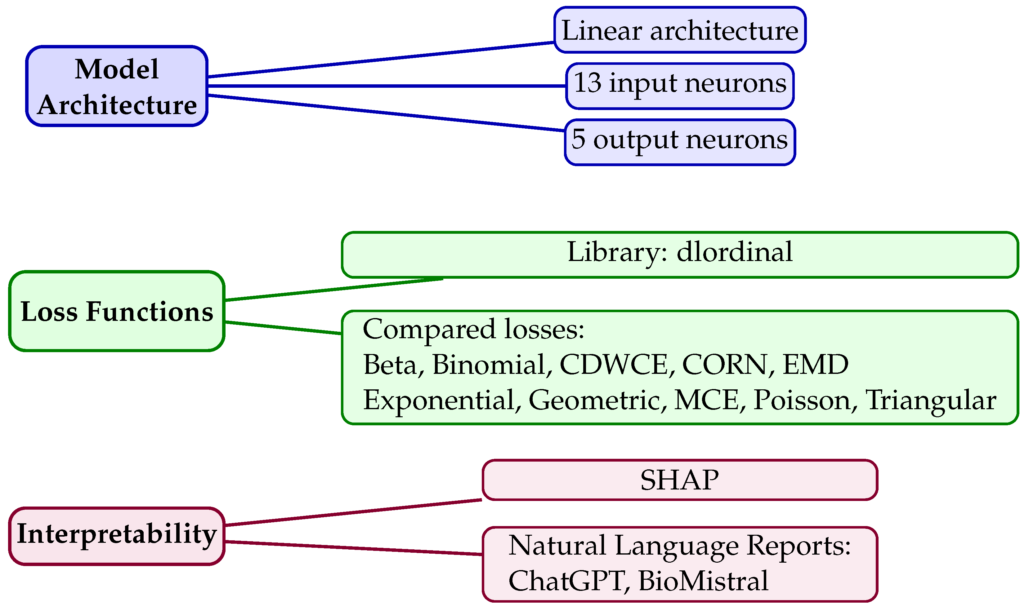
In this work, heart disease severity prediction is formulated as a five-class ordinal classification problem. The impact of different ordinal-aware loss functions is systematically evaluated using 10 loss functions [5,6,7,8,9,10,11,12,13], which are compared under a unified experimental framework using a linear model and repeated stratified cross-validation. By comparing standard accuracy, ordinal-aware metrics, extreme-class sensitivity measures, and interpretability outputs, this study provides evidence on how the choice of loss function affects not only overall predictive performance, but also the type of errors produced by the model. These findings can inform future healthcare model development by highlighting the need to select optimisation objectives according to the intended clinical use, particularly when errors involving distant or extreme severity classes are more clinically relevant. A diagram of the developed work is shown in Figure 1.

The results show that no single approach consistently outperformed all others across all metrics. Instead, different losses favoured different aspects of performance, including exact classification, ordinal proximity, extreme-class sensitivity, and probability-based error. This reinforces the importance of evaluating clinical severity prediction models using complementary metrics rather than relying on a single aggregate measure.

The main contributions of the present work include:

• A comprehensive evaluation of 10 loss functions for heart disease severity prediction using the Cleveland Heart Disease dataset.
• A unified experimental framework ensuring fair comparison across all losses, using the same linear model and cross-validation protocol.
• A performance analysis combining standard accuracy and ordinal evaluation metrics to assess both exact classification performance and ordinal consistency.
• An analysis of the trade-offs between global predictive performance, ordinal proximity, and sensitivity to extreme severity classes, with implications for clinical decision-support model development.
• Model interpretability with SHAP values and automatically generated reports.
• A discussion of how loss-function choice may influence future healthcare models, particularly in applications where clinically distant misclassifications should be penalized more strongly than near-miss errors.

The remainder of this paper is organized as follows. Section 2 reviews recent related work. Section 3 presents the dataset, the evaluated loss functions, and the evaluation methodology and metrics. Section 4 presents a correlation analysis between the features and the target variable, the results obtained with the different loss functions, an analysis of the error distribution, a SHAP-based interpretability analysis, and natural language reports generated by two different Large Language Models (LLMs). Finally, Section 5 concludes the paper by summarising the main findings, limitations, and directions for future work.

2. Related Work

Recent research on cardiovascular disease prediction has explored a broad range of machine learning approaches, including classical statistical models, hyperparameter tuned classifiers, federated learning, explainable AI, and emerging neural computing paradigms. A substantial part of this literature formulates heart disease prediction as a binary classification problem, typically distinguishing between the presence and absence of disease. Thakkar, Shukla and Patil [14] compared classical machine learning classifiers for robust heart disease prediction using the Cleveland dataset. Alsabhan and Alfadhly [15] performed a comparative study of several machine learning and deep learning models for heart disease diagnosis, with particular emphasis on preprocessing, feature scaling and binary disease detection. Wieckowska and Guzik [16] focused on the evaluation of binary classification models under balanced and imbalanced settings. These studies are relevant to the broader field of cardiovascular disease prediction. However, they mainly formulate the problem as binary diagnosis/classification.

Similarly, recent works on heart disease prediction using federated learning, hyperparameter tuning, and logistic regression generally approach the task as disease detection rather than severity estimation [17,18,19].

Other studies extend the methodological scope of medical classification by investigating model evaluation, scalability, few-shot learning, explainability, and alternative computational paradigms. Ghisoni et al. provided a large-scale comparison of quantum and classical neural networks in medical classification tasks [20], while Shysheya studied few-shot learning for both image classification and tabular data [21]. Explainability has also become increasingly prominent, as illustrated by the logic-based classification of biomedical data [22]. These works contribute to more transparent and robust medical AI systems but treat classification labels as either binary or nominal categories, without an inherent order.

Several recent works specifically address risk scoring, risk stratification, or clinical decision support. Chi and Birbil proposed an interpretable risk scoring system designed to maximise decision net benefit [23]. Alisoufi et al. presented a cost-aware and calibrated explainable AI framework for coronary artery disease risk stratification [24], while Kumar et al. developed and validated a clinical decision-support framework for heart disease prediction and risk reduction [25]. Karthikeya et al. also focused on deterministic and explainable preventive health risk stratification [26]. Although risk scores and risk strata naturally suggest ordered clinical states, these works are not necessarily framed as ordinal classification problems with explicit modelling of class order.

Another possible approach to severity prediction is regression, where the class labels are treated as numerical targets. This can be useful when the outcome represents a true continuous measurement or when equal spacing between target values is a reasonable assumption. However, in many clinical grading systems, severity levels are ordinal categories: they have a meaningful order, but the clinical distance between adjacent levels is not necessarily constant. Treating such labels as continuous values may therefore impose assumptions that are not fully supported by the data.

In contrast, ordinal classification explicitly assumes that the target labels follow a meaningful order, without necessarily imposing a continuous interpretation on the spacing between classes. XGBOrdinal extends XGBoost to ordinal data, showing that widely used machine learning models can be adapted to exploit class ordering [27].

Overall, the literature shows that cardiovascular disease prediction has been widely studied, but most works either formulate the task as binary classification or treat classes as nominal categories (

Table 1. Comparative summary of the analysed papers. Accuracy, AUC, sensitivity and F1 values are reported as percentages when applicable.

Paper	Problem Type	Results
Thakkar et al. (2020) [14]	Binary	AUC 93.00%
Alsabhan and Alfadhly (2025) [15]	Binary	Accuracy 90.20%
Więckowska et al. (2026) [16]	Binary	+16% AUC-PR improvement
Sorayaie et al. (2026) [17]	Binary	Accuracy 84.49%, Sensitivity 88.39%
Uddin et al. (2025) [18]	Binary	Accuracy 93.41%
Cahyono et al. (2026) [19]	Binary	Accuracy 82.20%
Ghisoni et al. (2026) [20]	Binary	Accuracy 87.46%
Shysheya (2025) [21]	Binary	AUC 91.00%
Nunkesser (2026) [22]	Nominal	F1 ≈ 30.00%
Chi et al. (2026) [23]	Binary	AUC 89.70%
Alisoufi et al. (2026) [24]	Binary	Accuracy 82.80%, Sensitivity 84.10%
Kumar et al. (2026) [25]	Binary	Accuracy 98.33%, Sensitivity 100%
Karthikeya et al. (2026) [26]	Nominal	Logical stability (no standard metrics)
Kahl et al. (2025) [27]	Ordinal	MAE 0.595, MSE 1.090

). Comparatively fewer studies explicitly preserve and exploit the ordered structure of disease severity labels. The present work addresses this gap by modelling heart disease severity prediction as a five-class ordinal classification problem and by comparing ten loss functions under a common experimental protocol.

3. Experimental Setup

3.1. Dataset

The Cleveland Heart Disease dataset [28] was used in this study. After removing missing values, the dataset contains 297 instances, 13 features and the target variable represents disease severity levels from 0 to 4 (

Table 2. Description of the Cleveland Heart Disease dataset features.

Feature	Description	Clinical Relevance
age	Age of the patient (years)	Increasing age is associated with higher cardiovascular risk.
sex	Sex (0 = female, 1 = male)	Males generally present higher risk of heart disease at earlier ages.
cp	Chest pain type (1: typical angina, 2: atypical angina, 3: non-anginal pain, 4: asymptomatic)	Types of chest pain are strongly related to the likelihood of coronary artery disease.
trestbps	Resting blood pressure (mmHg)	Elevated blood pressure (hypertension) is a major cardiovascular risk factor.
chol	Serum cholesterol (mg/dL)	High cholesterol levels are associated with increased risk of atherosclerosis.
fbs	Fasting blood sugar > 120 mg/dl (1 = true, 0 = false)	Elevated blood sugar may indicate diabetes, which increases cardiovascular risk.
restecg	Resting electrocardiographic results (0: normal, 1: ST-T abnormality, 2: left ventricular hypertrophy)	ECG abnormalities may indicate underlying cardiac dysfunction.
thalach	Maximum heart rate achieved	Lower maximum heart rate may indicate impaired cardiac function.
exang	Exercise-induced angina (1 = yes, 0 = no)	Presence of angina during exercise suggests myocardial ischemia.
oldpeak	ST depression induced by exercise relative to rest	Strong indicator of myocardial ischemia and disease severity.
slope	Slope of the peak exercise ST segment (1: upsloping, 2: flat, 3: downsloping)	Downsloping ST segment is associated with higher risk of heart disease.
ca	Number of major vessels (0–3) colored by fluoroscopy	Higher number of affected vessels indicates more severe disease.
thal	Thalassemia test result (3: normal, 6: fixed defect, 7: reversible defect)	Perfusion defects indicate abnormalities in blood flow to the heart muscle.
target	Heart disease severity level (0–4)	0 indicates absence of heart disease and higher values indicate increasing disease severity.

).

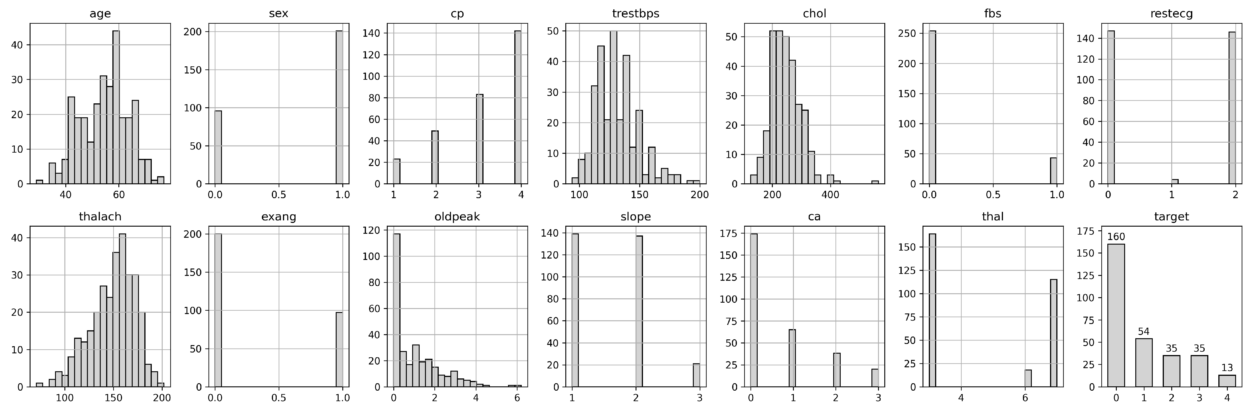
The 297 instances are distributed across the five ordinal severity levels as follows: class 0 with 160 samples, class 1 with 54 samples, class 2 with 35 samples, class 3 with 35 samples, and class 4 with 13 samples (Table 2). This confirms a class imbalance, with the absence-of-disease class being the most represented and the most severe class being under-represented (Figure 2). This imbalance must be considered when interpreting extreme-class sensitivity metrics since estimates for class 4 are based on a small number of observations.

Training features were normalized, in each iteration of the cross validation cycle, to have zero mean and one standard deviation. Test features of each iteration were also normalized, using the parameters derived in the train set.

3.2. Evaluated Ordinal Loss Functions

For the experiments, dlordinal [29] package was used. A linear model with 13 input neurons and 5 output neurons was used with different loss functions, listed in

Table 3. Loss functions.

Loss Function	Description	Formula	Reference
Beta	Beta-regularized cross-entropy	$-{\sum }_{k=1}^K{y}_{k,\mathrm{Beta}}^{*}log{\widehat{p}}_k$	[11]
Binomial	Binomial-smoothed cross-entropy	$-{\sum }_{k=1}^K{y}_{k,\mathrm{Bin}}^{*}log{\widehat{p}}_k$	[8]
CDWCE	Class-distance weighted cross-entropy	$-{\sum }_{k=1}^{K}w(y,k)log{\widehat{p}}_k$	[9]
CORN	Rank-consistent ordinal regression	$-{\sum }_{j=1}^{K-1}\left[z_{j}log{p}_j+(1-z_j)log(1-p_j)\right]$	[10]
EMD	Squared Earth Mover’s Distance	${\displaystyle \frac{1}{N}}{\sum }_{n=1}^N{\sum }_{k=1}^K{\left(F_{nk}-{\widehat{F}}_{nk}\right)}^2$	[7]
Exponential	Exponential-smoothed cross-entropy	$-{\sum }_{k=1}^K{y}_{k,\mathrm{Exp}}^{*}log{\widehat{p}}_k$	[12]
Geometric	Geometric label smoothing	$-{\sum }_{k=1}^K{y}_{k,\mathrm{Geo}}^{*}log{\widehat{p}}_k$	[6]
MCE	Mean Squared Error per class	${\displaystyle \frac{1}{NK}}{\sum }_{n=1}^N{\sum }_{k=1}^K{(y_{nk}-{\widehat{p}}_{nk})}^2$	[5]
Poisson	Poisson-smoothed cross-entropy	$-{\sum }_{k=1}^K{y}_{k,\mathrm{Pois}}^{*}log{\widehat{p}}_k$	[8]
Triangular	Triangular-smoothed cross-entropy	$-{\sum }_{k=1}^K{y}_{k,\mathrm{Tri}}^{*}log{\widehat{p}}_k$	[13]

N denotes the number of samples and K the number of classes. $y_{nk}$ and ${\widehat{p}}_{nk}$ represent the true and predicted probabilities for sample n and class k, respectively. For soft-label-based losses (Beta, Binomial, Exponential, Geometric, Poisson, and Triangular), the effective target distribution differs according to the smoothing distribution: $y_{k,d}^{*}=(1-\eta )y_k+\eta {\tilde{y}}_{k,d}$, where $y_k$ is the one-hot target label, ${\tilde{y}}_{k,d}$ is the soft-label distribution associated with distribution d, and $d\in \{\mathrm{Beta},\mathrm{Bin},\mathrm{Exp},\mathrm{Geo},\mathrm{Pois},\mathrm{Tri}\}$. In CDWCE, $w(y,k)={|y-k|}^{\alpha }$ denotes a distance-based weighting function that penalizes predictions proportionally to their ordinal distance from the true class. In CORN, $p_j$ is the conditional probability associated with binary ordinal sub-task j, and $z_j$ is the corresponding target. For EMD, $F_{nk}={\sum }_{i=1}^k{y}_{ni}$ and ${\widehat{F}}_{nk}={\sum }_{i=1}^k{\widehat{p}}_{ni}$ correspond to the cumulative true and predicted distributions, respectively. All loss-specific hyperparameters were set to their default values.

. All neural models were trained using the same optimisation protocol to ensure a controlled comparison across loss functions. The optimiser was Adam, with a learning rate of ${10}^{-3}$ and a maximum of 25 epochs. The batch size followed the default skorch NeuralNetClassifier setting. No internal validation split or early stopping was used. Training batches were shuffled during optimisation. The same training configuration was used for all loss functions and for all cross-validation folds. Loss-specific hyperparameters were kept at their default values in the dlordinal implementation.

3.3. Regression Baseline

To explicitly compare the ordinal classification formulation with a regression-based alternative, a regression baseline was also included. For this baseline, the heart disease severity label was treated as a numerical target and a linear regression model was trained using the same input features and the same validation protocol as the classification models.

Since the target variable represents five discrete severity levels, the continuous predictions produced by the regression model were converted back into valid class labels by rounding them to the nearest integer and clipping them to the interval $[0,4]$. The resulting predictions were then evaluated using the same metrics as the ordinal classification models.

This baseline was included to assess whether modelling the outcome as a continuous numerical variable provides competitive performance when compared with ordinal classification losses. However, unlike ordinal classification, this regression formulation implicitly assumes a metric interpretation of the target values, where the distances between consecutive severity levels are treated as approximately equal.

3.4. Sensitivity Analysis

The main comparison used a simple linear architecture in order to isolate the effect of the loss functions under a controlled setting. Using the same low-complexity model across all losses reduces the influence of architectural choices and allows the observed differences to be more directly associated with the optimisation objective.

To assess whether the observed trends were dependent on the linear architecture, an additional non-linear sensitivity analysis was performed using a multilayer perceptron (MLP). The MLP consisted of one hidden layer with 32 neurons and ReLU activation, followed by an output layer with five neurons corresponding to the severity classes. The same input features, preprocessing procedure, loss functions, optimiser, learning rate, batch size, number of epochs and validation protocol were used.

Because the dataset is imbalanced, particularly for the highest severity level, a balanced-training sensitivity analysis was performed (Appendix B). Random oversampling was applied only to the training data within each cross-validation fold, leaving the test folds unchanged. This avoids information leakage and allows the evaluation to reflect performance on the original data distribution. The aim of this analysis was to assess whether the relative behaviour of the loss functions remains stable when the minority severity classes are given greater influence during training.

3.5. Evaluation

Performance was evaluated using repeated stratified 5-fold cross-validation across 10 random seeds, resulting in 50 paired seed × fold evaluation blocks. For each seed, a stratified 5-fold split was generated, and all loss functions were evaluated using the same train–test partitions. Results are reported as mean and standard deviation across these repeated evaluation blocks. This protocol was used to reduce the influence of randomness due to fold assignment, data shuffling and model initialisation, which is particularly relevant given the limited sample size and class imbalance of the dataset.

Several metrics were used as summarized in

Table 4. Evaluation metrics.

Metric	Description	Goal	Formula	Reference
Accuracy	Standard accuracy	↑	${\displaystyle \frac{1}{N}}{\sum }_{i=1}^N\mathbf{1}({\widehat{y}}_i=y_i)$	Standard metric
Accuracy ± 1	Accuracy within one adjacent class	↑	${\displaystyle \frac{1}{N}}{\sum }_{i=1}^N\mathbf{1}\left(\right|{\widehat{y}}_i-y_i|\le 1)$	[30]
GMES	Geometric Mean Extreme-class Sensitivity	↑	$\sqrt{{\displaystyle \frac{T{P}_1}{T{P}_1+F{N}_1}}·{\displaystyle \frac{T{P}_K}{T{P}_K+F{N}_K}}}$	[30]
MES	Mean Extreme-class Sensitivity	↑	${\displaystyle \frac{1}{2}}\left({\displaystyle \frac{T{P}_1}{T{P}_1+F{N}_1}}+{\displaystyle \frac{T{P}_K}{T{P}_K+F{N}_K}}\right)$	[29]
Min Sensitivity	Minimum Sensitivity	↑	${min}_k{\displaystyle \frac{T{P}_k}{T{P}_k+F{N}_k}}$	[31]
AMAE	Average Mean Absolute Error	↓	${\displaystyle \frac{1}{K^{\prime }}}{\sum }_{k\in {\mathcal{K}}^{\prime }}{\displaystyle \frac{1}{N_k}}{\sum }_{i\in C_k}|{\widehat{y}}_i-y_i|$	[31]
MMAE	Maximum Mean Absolute Error	↓	${max}_{k\in {\mathcal{K}}^{\prime }}\left({\displaystyle \frac{1}{N_k}}{\sum }_{i\in C_k}|{\widehat{y}}_i-y_i|\right)$	[31]
RPS	Ranked Probability Score	↓	${\displaystyle \frac{1}{N}}{\sum }_{i=1}^N{\sum }_{k=1}^K{\left(F_{ik}-O_{ik}\right)}^2$	[32]

N denotes the total number of samples, K the number of classes, $N_k$ the number of samples in class k, and $C_k$ the set of samples belonging to class k. ${\widehat{y}}_i$ and $y_i$ denote the predicted and true class labels for sample i, respectively. ${\mathcal{K}}^{\prime }$ denotes the set of classes present in the test data since classes with no samples are removed when computing AMAE and MMAE. $T{P}_k$ and $F{N}_k$ denote the true positives and false negatives for class k. For RPS, $F_{ik}$ and $O_{ik}$ correspond to the cumulative predicted and true distributions for sample i and class k, respectively.

. Standard accuracy, accuracy within one adjacent class (Accuracy ± 1), Geometric Mean Extreme-class Sensitivity (GMES), Mean Extreme-class Sensitivity (MES), and Minimum Sensitivity (Min Sensitivity) are metrics whose values one wishes to maximize (↑). Average Mean Absolute Error (AMAE), Maximum Mean Absolute Error (MMAE), and Ranked Probability Score (RPS) are metrics whose values should be minimized (↓).

To statistically compare the evaluated loss functions, non-parametric paired tests were applied to the repeated cross-validation results. For each metric, the Friedman test was first used to assess whether significant global differences existed among the loss functions. When appropriate, post hoc pairwise comparisons were performed using the Wilcoxon signed-rank test with Holm correction for multiple comparisons. Since cross-validation folds are not fully independent, these statistical tests were interpreted as complementary evidence of robustness rather than as definitive proof of superiority.

4. Results

4.1. Correlation Analysis

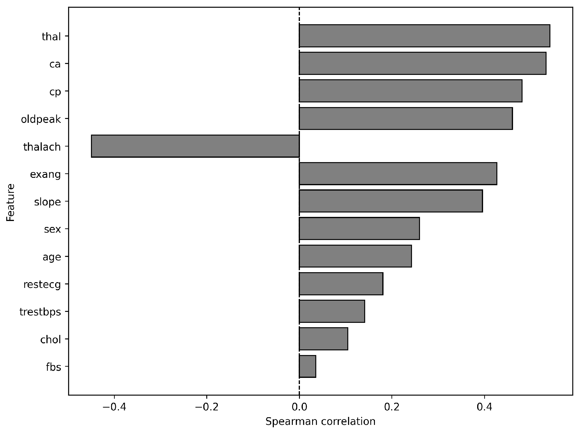
To assess the relationship between input features and disease severity, the Spearman correlation coefficient between each feature and the target variable is computed.

In Figure 3, it is visible that most features have positive correlations indicating that higher values of the feature are associated with more severe disease. The maximum heart rate achieved (feature thalach), as expected, shows a negative correlation, suggesting an inverse relationship.

The univariate monotonic associations between individual features and disease severity are generally modest. The strongest positive association is observed for thal, with a coefficient of approximately 0.54, while most remaining features show coefficients below 0.50. Therefore, these correlations should not be interpreted as evidence of strong individual predictors. Instead, they suggest that severity prediction is likely driven by the combined contribution of several clinical variables. This observation supports the use of multivariate machine learning models and motivates the subsequent SHAP-based analysis, which evaluates feature contributions in the context of the trained classifiers.

4.2. Loss Functions and Regression Baseline

Table 5. Results for metrics to maximize, reported as mean (standard deviation) across repeated stratified 5-fold cross-validation runs with multiple random seeds. Best numerical results are underlined.

Loss	Accuracy	Accuracy ± 1	GMES	MES	Min Sensitivity
Linear Regression	0.5159 (0.0612)	0.9199 (0.0249)	0.0000 (0.0000)	0.3262 (0.0517)	0.0000 (0.0000)
Beta	0.3188 (0.1334)	0.6253 (0.1364)	0.0484 (0.1664)	0.4817 (0.0569)	0.0264 (0.0683)
Binomial	0.3077 (0.1365)	0.6388 (0.1408)	0.0481 (0.1655)	0.4826 (0.0552)	0.0247 (0.0676)
CDWCE	0.3111 (0.1294)	0.6580 (0.1288)	0.0350 (0.1403)	0.4642 (0.0529)	0.0231 (0.0635)
CORN	0.1585 (0.0747)	0.4176 (0.1331)	0.0412 (0.1453)	0.4031 (0.0917)	0.0000 (0.0000)
EMD	0.2986 (0.1249)	0.6631 (0.1360)	0.0883 (0.2050)	0.4725 (0.0640)	0.0231 (0.0635)
Exponential	0.3141 (0.1364)	0.6364 (0.1416)	0.0484 (0.1664)	0.4839 (0.0556)	0.0313 (0.0771)
Geometric	0.3188 (0.1328)	0.6172 (0.1383)	0.0352 (0.1410)	0.4764 (0.0482)	0.0225 (0.0636)
MCE	0.2683 (0.1267)	0.5486 (0.1393)	0.0334 (0.1334)	0.4828 (0.0428)	0.0224 (0.0679)
Poisson	0.2168 (0.0874)	0.5352 (0.1286)	0.0220 (0.1088)	0.4782 (0.0377)	0.0144 (0.0401)
Triangular	0.3245 (0.1354)	0.6082 (0.1365)	0.0484 (0.1664)	0.4814 (0.0562)	0.0245 (0.0675)

and 

Table 6. Results for metrics to minimize, reported as mean (standard deviation) across repeated stratified 5-fold cross-validation runs with multiple random seeds. Best numerical results are underlined.

Loss	AMAE	MMAE	RPS
Linear Regression	0.8673 (0.1052)	1.8533 (0.4551)	0.5746 (0.0716)
Beta	1.3505 (0.3047)	2.0596 (0.5878)	9.8814 (3.5015)
Binomial	1.3457 (0.3212)	2.0089 (0.6304)	9.5041 (3.1866)
CDWCE	1.3267 (0.2834)	2.0721 (0.6037)	9.1325 (2.7738)
CORN	1.7996 (0.3021)	2.7485 (0.6079)	11.4992 (4.3468)
EMD	1.3244 (0.3078)	2.0745 (0.6710)	9.2292 (2.6675)
Exponential	1.3439 (0.3261)	1.9987 (0.6145)	9.5473 (3.2642)
Geometric	1.3725 (0.2987)	2.1265 (0.5975)	10.0024 (3.5926)
MCE	1.5031 (0.3259)	2.3381 (0.6731)	6.8375 (2.5543)
Poisson	1.5353 (0.2691)	2.3221 (0.5993)	9.1510 (2.8840)
Triangular	1.3745 (0.3010)	2.1437 (0.5854)	10.3813 (3.7691)

show the results for the metrics for which higher values are better and those for which lower values are better, respectively.

To complement the descriptive results, Friedman tests were applied to the paired seed × fold evaluation blocks. The corresponding results are reported in

Table 7. Friedman test results for the comparison of ordinal loss functions using the linear model. Tests were performed over paired seed × fold evaluation blocks. Kendall’s W is reported as an effect-size measure.

Metric	Blocks	Losses	${\mathit{\chi }}_{\mathit{F}}^2$	p-Value	Kendall’s W
Accuracy	50	10	255.6694	<0.001	0.5682
Accuracy ± 1	50	10	333.8615	<0.001	0.7419
GMES	50	10	10.4417	0.3159	0.0232
MES	50	10	173.9330	<0.001	0.3865
Min Sensitivity	50	10	21.2974	0.0114	0.0473
AMAE	50	10	226.5316	<0.001	0.5034
MMAE	50	10	170.1369	<0.001	0.3781
RPS	50	10	210.5760	<0.001	0.4679

. Post hoc Wilcoxon signed-rank comparisons with Holm correction were also performed when relevant. A filtered summary of the statistically significant pairwise comparisons is provided in Appendix C.

Results show:

• The linear regression baseline achieved the highest standard accuracy and accuracy ± 1, indicating the best overall exact agreement and the highest proportion of predictions within one adjacent severity level after rounding the continuous predictions to the nearest valid class.
• The linear regression baseline also achieved the lowest AMAE, MMAE and RPS. However, its GMES and Min Sensitivity were both zero, indicating poor identification of samples from the extreme severity classes.
• Among the ordinal classification losses, Triangular obtained the highest standard Accuracy, while EMD achieved the highest accuracy ± 1 and GMES.
• Exponential achieved the highest MES and Min Sensitivity among the ordinal classification losses, suggesting comparatively better behaviour for sensitivity-related metrics.
• For the metrics to minimize, EMD obtained the lowest AMAE among the ordinal losses, exponential obtained the lowest MMAE, and MCE obtained the lowest RPS.

These results highlight a trade-off between global predictive performance and sensitivity to clinically relevant extreme classes. The linear regression baseline performed best according to aggregate metrics such as standard accuracy, accuracy ± 1, AMAE, MMAE and RPS. This suggests that treating severity labels as numerical targets can produce predictions that are, on average, close to the true severity level. However, the same baseline obtained zero GMES and zero Min Sensitivity, showing that high aggregate performance does not necessarily imply adequate recognition of the most extreme severity classes.

The ordinal classification losses showed a different pattern. Although none of them surpassed the linear regression baseline in standard Accuracy or Accuracy ± 1, some ordinal losses achieved better sensitivity-related behaviour for the extreme classes. In particular, EMD obtained the highest GMES, while exponential achieved the highest MES and Min sensitivity among the ordinal classification losses. This suggests that ordinal-aware losses may provide complementary advantages in imbalanced clinical ordinal prediction tasks, especially when performance on less frequent severity levels is considered important.

The Friedman test results further support the interpretation that the choice of loss function affects model behaviour across most evaluation metrics. Statistically significant global differences were observed for Accuracy, Accuracy ± 1, MES, Min Sensitivity, AMAE, MMAE and RPS. In contrast, GMES did not show a statistically significant global difference, which is consistent with the high variability and frequent zero values observed for this metric. Therefore, the statistical results should be interpreted together with the descriptive performance values, rather than as evidence of universal superiority of any single loss function.

Several loss functions obtained zero or near-zero GMES or Min Sensitivity values, indicating difficulties in correctly identifying samples from extreme classes. This behaviour is likely related to the strong class imbalance present in the dataset, namely the severe under-representation of heart disease severity level 4. Therefore, the results should be interpreted not only in terms of overall accuracy, but also in terms of class-wise sensitivity and ordinal error behaviour.

When looking at the state-of-the-art results, comparison is only possible with [27] since it is the only one that frames the problem as ordinal classification. Although XGBOrdinal [27] reported lower MAE values than those obtained in the present study, direct comparison is not straightforward due to differences in the experimental protocols. Namely, [27] used a random train–test split, while the present work employs repeated stratified 5-fold cross-validation across multiple random seeds. Furthermore, the goal of the present study is to assess different loss functions and, therefore, only a simple linear model is used, whereas XGBOrdinal relies on gradient-boosted decision trees specifically designed for ordinal prediction.

Since no single ordinal loss function dominated all metrics, EMD, Exponential, MCE and Triangular were retained for the remaining error-distribution and interpretability analyses. These losses represent complementary behaviours among the evaluated ordinal classification approaches: Triangular obtained the highest standard accuracy, EMD achieved the highest accuracy ± 1 and GMES, Exponential obtained the highest MES and Min sensitivity, and MCE achieved the lowest RPS among the ordinal classification losses. This selection allows the subsequent analyses to compare losses with distinct optimisation behaviours rather than focusing on a single performance criterion.

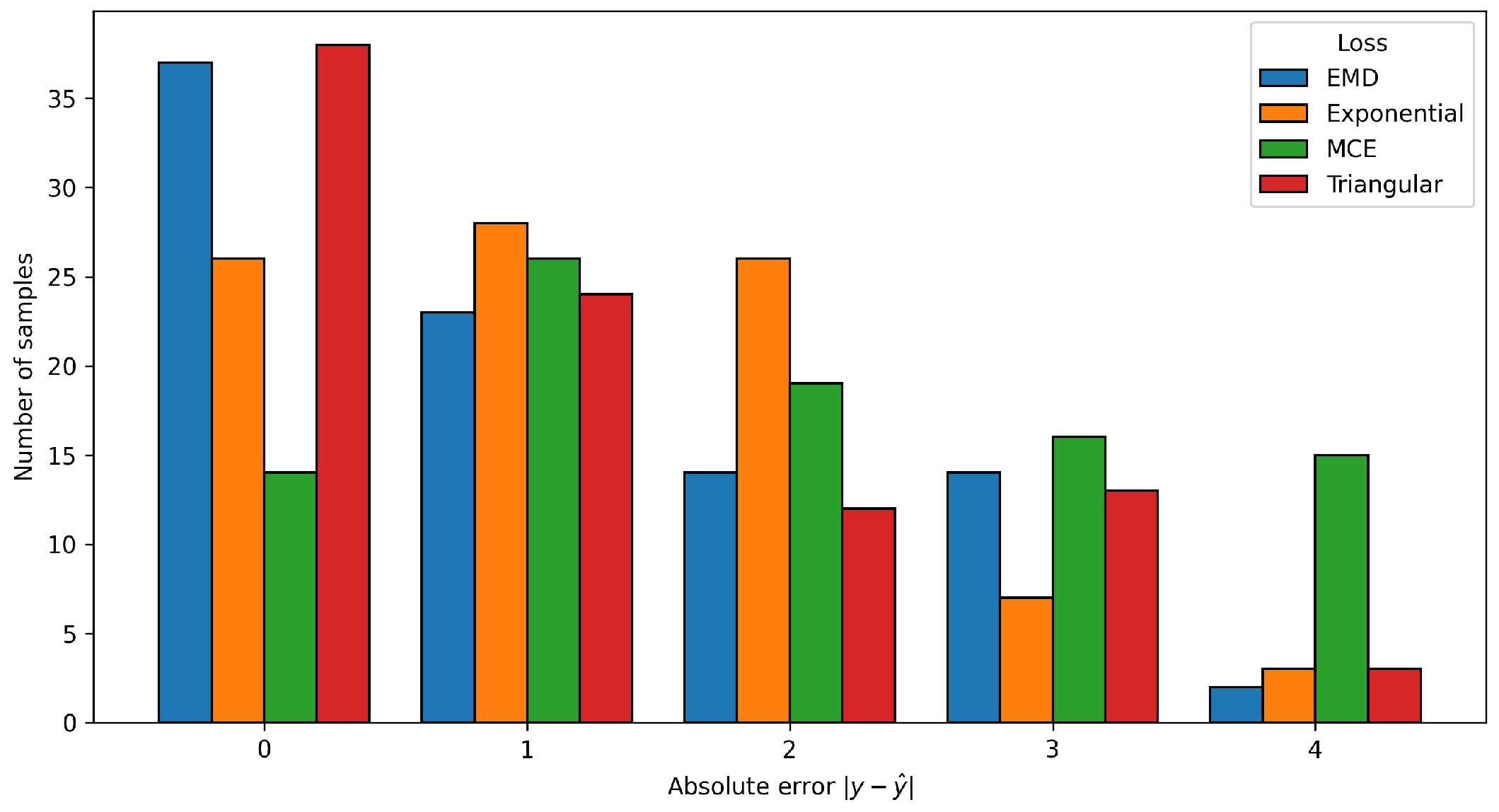
4.3. Error Distribution Analysis

Figure 4 presents the distribution of absolute prediction errors across the selected loss functions. The figure illustrates the role of ordinal losses in encouraging predictions that remain closer to the true class, particularly by reducing large ordinal deviations. This behaviour is reflected in the progressive decrease in the number of samples as the absolute error increases, indicating that predictions tend to remain within neighbouring severity levels rather than distant classes.

4.4. Feature Relevance

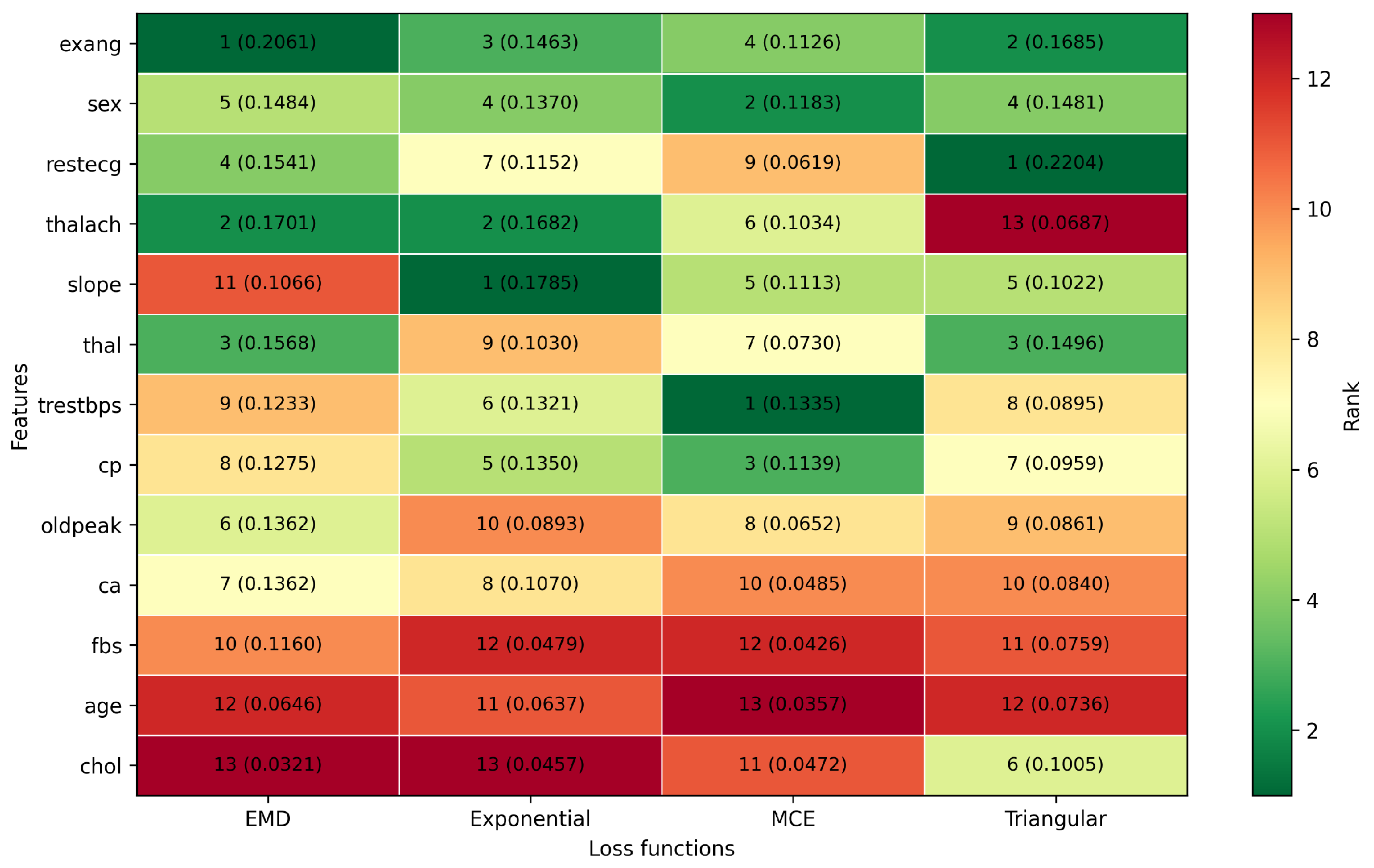
To assess whether the choice of loss function influences model-based feature relevance, SHapley Additive exPlanations (SHAP) [33] was used to compute the mean importance of each feature. Figure 5 presents the SHAP-based feature rankings across the selected ordinal loss functions, with the corresponding mean absolute SHAP importance values shown in parentheses. The complete numerical values are provided in Appendix A. Some differences in rank correspond to small differences in SHAP magnitude and should therefore be interpreted cautiously, particularly given the limited and imbalanced nature of the dataset.

Although the Spearman correlation analysis presented in Figure 3 highlights variables such as thal and ca as strongly associated with the target variable, the model-based feature importance analysis reveals a different ranking. Across the selected losses, features such as thalach, sex, cp, and exang show the highest mean absolute SHAP importance values. This suggests that feature relevance in the trained models is not determined solely by univariate association with the target but also by the multivariate contribution of each variable, the optimisation criterion induced by each loss function, and the way information is distributed across correlated predictors.

This distinction is particularly important in clinical datasets, where several variables may capture partially overlapping aspects of cardiovascular risk. For example, variables related to exercise response, chest pain, perfusion defects, and vessel involvement may not contribute independently to the model. In the presence of correlated or clinically related predictors, SHAP importance can be distributed across multiple features, meaning that a variable with a high univariate correlation may receive only moderate model-based importance if its information is partly captured by other predictors. This may help explain why ca, despite exhibiting a high Spearman correlation with the target, does not appear among the most important SHAP-ranked features.

The SHAP analysis should therefore be interpreted as an explanation of model behaviour rather than as direct evidence of clinical causality. The results indicate which variables were most influential for the trained models under each loss function, but they do not establish independent causal effects or quantify clinical interactions directly. A more detailed investigation of feature interactions, multicollinearity, and clinical validity would require additional analyses and expert clinical assessment. Nevertheless, the observed differences between correlation-based relevance and SHAP-based relevance reinforce the importance of combining univariate, multivariate, and interpretability analyses when evaluating clinical decision-support models.

4.5. Sensitivity Analysis

To evaluate whether the observed differences between loss functions were dependent on the use of a linear architecture, a non-linear sensitivity analysis was performed using a multilayer perceptron.

Table 8. Non-linear sensitivity analysis using a multilayer perceptron. Results are presented as mean (standard deviation) for metrics to maximize. Best results are underlined.

Loss	Accuracy	Accuracy ± 1	GMES	MES	Min Sensitivity
Beta	0.5755 (0.0335)	0.8087 (0.0360)	0.0000 (0.0000)	0.5000 (0.0000)	0.0000 (0.0000)
Binomial	0.5563 (0.0534)	0.8195 (0.0380)	0.0000 (0.0000)	0.5000 (0.0000)	0.0000 (0.0000)
CDWCE	0.5667 (0.0575)	0.8323 (0.0409)	0.0000 (0.0000)	0.4997 (0.0022)	0.0000 (0.0000)
CORN	0.1239 (0.0423)	0.5219 (0.1131)	0.0000 (0.0000)	0.4831 (0.0294)	0.0000 (0.0000)
EMD	0.5411 (0.0857)	0.7963 (0.0406)	0.0000 (0.0000)	0.4994 (0.0031)	0.0000 (0.0000)
Exponential	0.5704 (0.0452)	0.8269 (0.0376)	0.0000 (0.0000)	0.5000 (0.0000)	0.0000 (0.0000)
Geometric	0.5842 (0.0376)	0.8135 (0.0391)	0.0000 (0.0000)	0.5000 (0.0000)	0.0000 (0.0000)
MCE	0.5731 (0.0437)	0.8175 (0.0410)	0.0000 (0.0000)	0.5000 (0.0000)	0.0047 (0.0237)
Poisson	0.3399 (0.0521)	0.8115 (0.0410)	0.0000 (0.0000)	0.5000 (0.0000)	0.0275 (0.0694)
Triangular	0.5798 (0.0352)	0.8034 (0.0385)	0.0000 (0.0000)	0.5000 (0.0000)	0.0000 (0.0000)

and 

Table 9. Non-linear sensitivity analysis using a multilayer perceptron. Results are presented as mean (standard deviation) for metrics to minimize. Best results are underlined.

Loss	AMAE	MMAE	RPS
Beta	1.4168 (0.1848)	2.8217 (0.5698)	5.5643 (1.7693)
Binomial	1.3411 (0.1774)	2.6994 (0.5257)	4.0598 (1.2888)
CDWCE	1.2882 (0.1908)	2.6324 (0.5322)	4.5855 (1.6489)
CORN	1.9155 (0.2224)	3.4781 (0.4487)	8.2984 (2.5033)
EMD	1.4617 (0.2108)	2.8514 (0.6085)	5.0116 (1.6194)
Exponential	1.2861 (0.1828)	2.5541 (0.5819)	3.9756 (1.4177)
Geometric	1.3550 (0.1973)	2.6488 (0.6253)	5.8194 (1.9022)
MCE	1.2437 (0.1817)	2.3274 (0.6016)	0.8602 (0.1811)
Poisson	1.1638 (0.1862)	2.0690 (0.6133)	4.3930 (1.3937)
Triangular	1.4306 (0.2178)	2.7955 (0.6367)	7.0183 (2.3366)

report the corresponding results for the metrics to maximize and minimize, respectively.

The MLP sensitivity analysis showed that the relative behaviour of the losses changed when a non-linear architecture was used. Geometric achieved the highest standard accuracy, while CDWCE achieved the highest accuracy ± 1. For the metrics to minimize, Poisson obtained the lowest AMAE and MMAE, whereas MCE achieved the lowest RPS.

However, the MLP did not substantially improve the identification of extreme severity classes. All losses obtained zero GMES, and most losses also obtained zero Min Sensitivity. Only MCE and Poisson achieved non-zero Min Sensitivity values, although these remained low. This suggests that the difficulty in predicting the minority extreme classes is not only related to the linear architecture but is also strongly influenced by the limited and imbalanced nature of the dataset.

Overall, the sensitivity analysis confirms that the ranking of loss functions may depend on the model architecture. Nevertheless, the main conclusion remains unchanged: no single loss function consistently dominates all evaluation criteria, and the choice of loss should be guided by the clinical objective of interest, such as exact classification, ordinal proximity, probability-based error, or sensitivity to extreme severity classes.

As an additional sensitivity analysis, random oversampling was applied within the training folds to assess whether the relative behaviour of the loss functions remained stable when minority severity classes were given greater influence during training. The oversampling procedure was applied only to the training data in each cross-validation fold, while the corresponding test fold was left unchanged. This avoids information leakage and preserves the original class distribution during evaluation. The results of this analysis are reported in Appendix B.

4.6. Natural Language Explanations

SHAP values were used as structured input to large language models, together with the predicted severity class. This strategy aimed to translate feature-level contributions into concise natural language explanations while preserving the original classifier as the source of the prediction. The generic prompt is presented in Listing 1.

Two Large Language Models (LLMs) were considered: a general-purpose model, ChatGPT (OpenAI, GPT-5.5 Thinking, version used in June 2026), and a biomedical-domain model, BioMistral. BioMistral [34] is an open-source LLM tailored for biomedical applications, using Mistral as its foundation model and further pre-trained on PubMed Central. Representative examples of natural language explanations generated for the MCE loss are presented in

Table 10. Examples of natural language explanations generated from SHAP values for MCE predictions.

Classifications	Prompt	ChatGPT	BioMistral
True label 4, predicted as 4	You are a medical AI assistant helping to explain a machine learning prediction. The model predicted heart disease severity class 4. The following SHAP values indicate the contribution of each feature to the prediction: - ca: SHAP value = 0.1664 - oldpeak: SHAP value = 0.1539 - thal: SHAP value = 0.1296 - thalach: SHAP value = 0.1279 - cp: SHAP value = 0.1275 Write a short clinical explanation in natural language. Requirements: - Explain which features contributed most to the prediction. - Distinguish features increasing severity from features decreasing severity. - Do not recommend treatment. - Use cautious clinical language.	The prediction of heart disease severity class 4 appears to have been driven mainly by the features ca, oldpeak, thal, thalach, and cp. Among these, the strongest contributors were ca (number of major vessels visualized) and oldpeak (ST depression during exercise), both of which increased the likelihood of a more severe classification. Elevated contributions from these variables may reflect a greater burden of underlying cardiovascular abnormality. The variables thal and cp (chest pain type) also contributed positively to the prediction, suggesting that the observed patterns were more consistent with higher disease severity. In addition, thalach (maximum heart rate achieved) influenced the model substantially; depending on the underlying measured value, this feature may either support or reduce the probability of severe disease. In this prediction, its contribution was aligned with greater severity. Overall, the combination of these features led the model to associate the clinical profile with a higher-risk pattern consistent with severity class 4.	The patient’s age, peak creatine kinase level, thalassemia status, resting heart rate, and cholesterol level were the main features that contributed to the prediction of heart disease severity class 4. The patient’s age and peak creatine kinase level were found to increase the severity of heart disease, while the patient’s resting heart rate, thalassemia status, and cholesterol level were found to decrease the severity of heart disease.
True label 4, predicted as 0	You are a medical AI assistant helping to explain a machine learning prediction. The model predicted heart disease severity class 0. The following SHAP values indicate the contribution of each feature to the prediction: - ca: SHAP value = 0.2327 - exang: SHAP value = 0.1841 - thal: SHAP value = 0.1200 - restecg: SHAP value = 0.1198 - age: SHAP value = 0.1195 Write a short clinical explanation in natural language. Requirements: - Explain which features contributed most to the prediction. - Distinguish features increasing severity from features decreasing severity. - Do not recommend treatment. - Use cautious clinical language.	The prediction of heart disease severity class 0 appears to have been influenced most strongly by the variables ca and exang, which showed the largest SHAP contributions. In this context, these features likely contributed toward a lower predicted severity classification. The features thal, restecg, and age also contributed meaningfully to the model output, although to a lesser extent. Overall, the combination of these variables appears to have shifted the prediction toward class 0 rather than toward a higher severity category. Features with positive SHAP contributions supported the predicted class, whereas features with negative SHAP contributions (if present but not listed here) would have pushed the prediction toward greater disease severity. This interpretation reflects the model’s statistical reasoning and should be considered alongside the broader clinical context.	The model predicted heart disease severity class 0. The features that contributed most to the prediction were: (1) chest pain (SHAP value = 0.2327), (2) exang (SHAP value = 0.1841), (3) thal (SHAP value = 0.1200), (4) restecg (SHAP value = 0.1198), and (5) age (SHAP value = 0.1195).

.

Listing 1. Generic prompt used for generating natural language explanations.

You are a medical AI assistant helping to explain a machine learning prediction.   The model predicted heart disease severity class {predicted_class}.   The following SHAP values indicate the contribution of each feature to the prediction: {shap_values_text}   Write a short clinical explanation in natural language.   Requirements: - Explain which features contributed most to the prediction. - Distinguish features increasing severity from features decreasing severity. - Do not recommend treatment. - Use cautious clinical language.

The examples reported in this section should be interpreted as illustrative outputs rather than as clinically validated explanations. They show how SHAP values can be translated into natural language narratives, but they do not constitute an objective validation of explanation quality, reliability, or clinical usefulness. A systematic evaluation of generated explanations would require a dedicated assessment protocol, including review by clinical experts, factuality checks to verify whether the narrative accurately reflects the input SHAP values, consistency analysis across repeated generations, and human ratings of clarity, usefulness and potential clinical safety. Such an evaluation is necessary before these explanations can be considered reliable for clinical decision-support applications.

In the illustrative examples analysed, ChatGPT generated more coherent explanations than BioMistral. ChatGPT more explicitly linked the SHAP values to the predicted class and provided a clearer interpretation of feature contributions. In contrast, BioMistral sometimes produced superficial or inaccurate explanations, including confusion between feature meanings and repetition of the input SHAP values without a clear explanation of their contribution to the prediction. However, these observations are qualitative and based on selected examples. Therefore, they should not be interpreted as a systematic comparison between LLMs. Instead, they highlight the need for formal evaluation protocols before LLM-generated explanations are used in medical decision-support contexts.

5. Conclusions

This study compared several ordinal loss functions for heart disease severity prediction using the Cleveland Heart Disease dataset. The results show that different optimisation objectives favour different aspects of model performance, including exact classification, ordinal proximity, probability-based error, and sensitivity to extreme severity classes. The additional regression baseline and MLP sensitivity analysis further showed that the ranking of methods can change depending on the modelling formulation and architecture. Therefore, no single loss function or model formulation should be considered uniformly superior across all evaluation criteria. Accordingly, the present study should be interpreted as a controlled analysis of ordinal-loss behaviour on one clinical ordinal dataset, rather than as a definitive benchmark across all ordinal medical prediction tasks. The Friedman tests indicated statistically significant global differences for most metrics, but not for GMES, reinforcing the need to interpret numerical differences cautiously and in relation to the specific clinical objective being considered.

The main limitation of this study is the use of a relatively small and imbalanced dataset, which may particularly affect the estimation of sensitivity for extreme severity classes. Although a balanced-training analysis using random oversampling was performed, this represents only one simple strategy for addressing class imbalance. Other approaches, such as class-weighted optimisation, synthetic oversampling methods, cost-sensitive learning, or clinically informed sampling strategies, may lead to different behaviour and should be explored in future work.

Another limitation concerns the evaluation of the natural language explanations generated from SHAP values. In this study, these explanations were included as illustrative examples and were not systematically validated by clinical experts or through objective factuality, consistency, or human-rating metrics. Therefore, they should not be interpreted as clinically validated explanations.

The interpretation of the comparative results should also consider two methodological constraints. First, the statistical tests were conducted over repeated cross-validation blocks from a relatively small and imbalanced dataset. Although repeated seeds improve robustness, cross-validation folds are not fully independent, and the statistical results should therefore be interpreted as complementary evidence. Second, loss-specific hyperparameter tuning was not performed. All losses were trained under a common optimisation protocol to support a controlled comparison, but different losses may have different optimisation landscapes and may benefit from different learning rates, regularisation settings, or loss-specific hyperparameters. Future work should therefore investigate loss-specific tuning strategies and assess whether the relative ranking of losses remains stable under individually optimised configurations.

Possible avenues for future work include:

• Validation on larger and more balanced clinical datasets to obtain more reliable estimates of performance for rare extreme severity classes.
• Further evaluation of additional model architectures and larger ordinal clinical datasets, since the present study only included one non-linear sensitivity analysis.
• Further investigation of imbalance-aware learning strategies, including class-weighted optimisation, synthetic oversampling, cost-sensitive learning, and clinically informed sampling approaches [35,36].
• Extension to medical imaging data (e.g., MRI and CT [37,38]).
• Development of a systematic evaluation framework for generated clinical explanations, including clinical expert review, factuality assessment against the input SHAP values, consistency analysis across repeated generations, and human ratings of clarity, usefulness and potential clinical safety.

References

- Maurício, J.; Domingues, I.; Oliveira, H. Diagnosing Ulcerative Colitis Severity through Image Analysis Using Ordinal Classification. In Proceedings of the Portuguese Conference on Pattern Recognition (RecPad), Aveiro, Portugal, 31 October 2025. [Google Scholar]
- Amorim, J.P.; Domingues, I.; Abreu, P.H.; Santos, J. Interpreting Deep Learning Models for Ordinal Problems. In Proceedings of the European Symposium on Artificial Neural Networks, Computational Intelligence and Machine Learning, Bruges, Belgium, 25–27 April 2018. [Google Scholar]
- Domingues, I.; Cardoso, J.S. Max-Ordinal Learning. IEEE Trans. Neural Netw. Learn. Syst. 2013, 25, 1384–1389. [Google Scholar] [CrossRef] [Scilit]
- Cardoso, J.S.; Sousa, R.; Domingues, I. Ordinal Data Classification Using Kernel Discriminant Analysis: A Comparison of Three Approaches. In Proceedings of the 11th International Conference on Machine Learning and Applications, Boca Raton, FL, USA, 12–15 December 2012. [Google Scholar]
- Bishop, C.M. Pattern Recognition and Machine Learning; Information Science and Statistics; Springer: New York, NY, USA, 2006. [Google Scholar]
- Haas, S.; Hüllermeier, E. Rectifying Bias in Ordinal Observational Data Using Unimodal Label Smoothing. In Proceedings of the Machine Learning and Knowledge Discovery in Databases: Applied Data Science and Demo Track—European Conference, ECML PKDD 2023, Turin, Italy, September 18–22, 2023, Proceedings, Part VI; Morales, G.D.F., Perlich, C., Ruchansky, N., Kourtellis, N., Baralis, E., Bonchi, F., Eds.; Lecture Notes in Computer Science; Springer: Berlin/Heidelberg, Germany, 2023; Volume 14174, pp. 3–18. [Google Scholar] [CrossRef] [Scilit]
- Hou, L.; Yu, C.; Samaras, D. Squared Earth Mover’s Distance-based Loss for Training Deep Neural Networks. arXiv 2016, arXiv:1611.05916. [Google Scholar] [CrossRef] [Scilit]
- Liu, X.; Fan, F.; Kong, L.; Diao, Z.; Xie, W.; Lu, J.; You, J. Unimodal Regularized Neuron Stick-breaking for Ordinal Classification. Neurocomputing 2020, 388, 34–44. [Google Scholar] [CrossRef] [Scilit]
- Polat, G.; Ergenc, I.; Kani, H.T.; Alahdab, Y.O.; Atug, O.; Temizel, A. Class distance weighted cross-entropy loss for ulcerative colitis severity estimation. In Proceedings of the Annual Conference on Medical Image Understanding and Analysis; Springer: Berlin/Heidelberg, Germany, 2022; pp. 157–171. [Google Scholar] [CrossRef] [Scilit]
- Shi, X.; Cao, W.; Raschka, S. Deep neural networks for rank-consistent ordinal regression based on conditional probabilities. Pattern Anal. Appl. 2023, 26, 941–955. [Google Scholar] [CrossRef] [Scilit]
- Vargas, V.M.; Gutiérrez, P.A.; Hervás-Martínez, C. Unimodal regularisation based on beta distribution for deep ordinal regression. Pattern Recognit. 2022, 122, 108310. [Google Scholar] [CrossRef] [Scilit]
- Vargas, V.M.; Gutiérrez, P.A.; Rosati, R.; Romeo, L.; Frontoni, E.; Hervás-Martínez, C. Exponential loss regularisation for encouraging ordinal constraint to shotgun stocks quality assessment. Appl. Soft Comput. 2023, 138, 110191. [Google Scholar] [CrossRef] [Scilit]
- Vargas, V.M.; Gutiérrez, P.A.; Barbero-Gómez, J.; Hervás-Martínez, C. Soft labelling based on triangular distributions for ordinal classification. Inf. Fusion 2023, 93, 258–267. [Google Scholar] [CrossRef] [Scilit]
- Kumar Thakkar, H.; Shukla, H.; Patil, S. A Comparative Analysis of Machine Learning Classifiers for Robust Heart Disease Prediction. In Proceedings of the IEEE 17th India Council International Conference (INDICON); IEEE: New York, NY, USA, 2020; pp. 1–6. [Google Scholar] [CrossRef] [Scilit]
- Alsabhan, W.; Alfadhly, A. Effectiveness of Machine Learning Models in Diagnosis of Heart Disease: A Comparative Study. Sci. Rep. 2025, 15, 24568. [Google Scholar] [CrossRef] [Scilit] [PubMed]
- Więckowska, B.; Guzik, P. Usmile likelihood evaluation provides robust threshold free assessment of binary classification models for balanced and imbalanced datasets. Sci. Rep. 2026, 16, 10000. [Google Scholar] [CrossRef] [Scilit] [PubMed]
- Sorayaie Azar, A.; Gholami, F.; Sharifi, L.; Asl Asgharian Sardroud, A.; Bagherzadeh Mohasefi, J.; Wiil, U.K. FMLCA: Explainable and privacy-preserving federated machine learning classification algorithms for predicting heart disease in patients. Eur. J. Med. Res. 2026, 31, 423. [Google Scholar] [CrossRef] [Scilit]
- Uddin, N.; Hossain, M.S.; Mahmud, M.Z.; Ferdous, R.; Talukder, M.A. HPML-CVD: Hyperparameter tuned machine learning model to predict cardiovascular disease. Biomed. Mater. Devices 2026, 4, 861–875. [Google Scholar]
- Cahyono, A.; Ameriza, I.; Gunadi, G.; Syifa, E.D.A.; Alqudah, M.K. Calibration and Applied Statistical Modeling Using Logistic Regression on the UCI Heart Disease Dataset. J. Appl. Inform. Comput. 2026, 10, 327–335. [Google Scholar] [CrossRef] [Scilit]
- Ghisoni, F.; Borrotti, M.; Mariani, P. A large scale statistical analysis of quantum and classical neural networks in the medical domain. Sci. Rep. 2026, 16, 3719. [Google Scholar] [CrossRef] [Scilit] [PubMed]
- Shysheya, A. Advances in Few-Shot Learning for Image Classification and Tabular Data. Ph.D. Thesis, University of Cambridge, Cambridge, UK, 2025. [Google Scholar] [CrossRef]
- Nunkesser, R. A logicGP Trainer for Classification of Biomedical Data. In Proceedings of the 19th International Joint Conference on Biomedical Engineering Systems and Technologies—Volume 2: BIOINFORMATICS. INSTICC; SciTePress: Setúbal, Portugal, 2026; pp. 609–616. [Google Scholar] [CrossRef] [Scilit]
- Chi, W.; Birbil, Ş.İ. Learning An Interpretable Risk Scoring System for Maximizing Decision Net Benefit. arXiv 2026, arXiv:2604.04241. [Google Scholar]
- Alisoufi, M.; Dehvari, S.; Heidari, S.; Mohebbi, N.; Jafarpour Sadegh, A.; Eshragh Abad Shapori, P. A Cost-Aware and Calibrated Explainable AI Framework for Equitable Coronary Artery Disease Risk Stratification Using Minimal Clinical Data. Infosci. Trends 2026, 3, 80–104. [Google Scholar] [CrossRef] [Scilit]
- Kumar, R.; Yadav, P.; Kilambi, S.; Banavar, M. Development and validation of the Sriya Expert Index Plus (SXI++) framework for heart disease prediction and risk reduction through clinical decision support. J. Med. Artif. Intell. 2026, 9, 11. [Google Scholar] [CrossRef] [Scilit]
- Karthikeya, M.V.; Nagalakshmi, T.V.; Kishore, D.N.; Sagar, M. An Explainable Deterministic Framework for Preventive Health Risk Stratification with Multilingual Decision Support for Low-Resource Environments. Indian J. Comput. Sci. Technol. 2026, 5, 160–168. [Google Scholar] [CrossRef] [Scilit]
- Kahl, F.; Kahl, I.; Jonas, S.M. XGBOrdinal: An XGBoost Extension for Ordinal Data. In Intelligent Health Systems–From Technology to Data and Knowledge; IOS Press: Amsterdam, The Netherlands, 2025; pp. 462–466. [Google Scholar]
- Detrano, R.; Janosi, A.; Steinbrunn, W.; Pfisterer, M.; Schmid, J.-J.; Sandhu, S.; Guppy, K.H.; Lee, S.; Froelicher, V. International Application of a New Probability Algorithm for the Diagnosis of Coronary Artery Disease. Am. J. Cardiol. 1989, 64, 304–310. [Google Scholar] [CrossRef] [Scilit] [PubMed]
- Bérchez-Moreno, F.; Ayllón-Gavilán, R.; Vargas-Yun, V.M.; Guijo-Rubio, D.; Hervás-Martínez, C.; Fernández, J.C.; Gutiérrez, P.A. dlordinal: A Python package for deep ordinal classification. Neurocomputing 2025, 622, 129305. [Google Scholar] [CrossRef] [Scilit]
- Vargas, V.M.; Gutiérrez, P.A.; Barbero-Gómez, J.; Hervás-Martínez, C. Improving the classification of extreme classes by means of loss regularisation and generalised beta distributions. arXiv 2024, arXiv:2407.12417. [Google Scholar] [CrossRef] [Scilit]
- Cruz-Ramirez, M.; Hervas-Martinez, C.; Sanchez-Monedero, J.; Gutierrez, P.A. Metrics to guide a multi-objective evolutionary algorithm for ordinal classification. Neurocomputing 2014, 135, 21–31. [Google Scholar] [CrossRef] [Scilit]
- Janitza, S.; Tutz, G.; Boulesteix, A.L. Random forest for ordinal responses: Prediction and variable selection. Comput. Stat. Data Anal. 2016, 96, 57–73. [Google Scholar] [CrossRef] [Scilit]
- Lundberg, S.M.; Lee, S.I. A Unified Approach to Interpreting Model Predictions. In Proceedings of the Advances in Neural Information Processing Systems 30 (NeurIPS 2017); NeurIPS: Sydney, Australia, 2017; pp. 4765–4774. [Google Scholar]
- Labrak, Y.; Bazoge, A.; Morin, E.; Gourraud, P.A.; Rouvier, M.; Dufour, R. BioMistral: A Collection of Open-Source Pretrained Large Language Models for Medical Domains. arXiv 2024, arXiv:2402.10373. [Google Scholar] [CrossRef] [Scilit]
- Marques, F.; Duarte, H.; Santos, J.; Domingues, I.; Amorim, J.P.; Abreu, P.H. An Iterative Oversampling Approach for Ordinal Classification. In Proceedings of the 34th ACM/SIGAPP Symposium on Applied Computing; Association for Computing Machinery: New York, NY, USA, 2019. [Google Scholar]
- Domingues, I.; Amorim, J.P.; Abreu, P.H.; Duarte, H.; Santos, J. Evaluation of Oversampling Data Balancing Techniques in the Context of Ordinal Classification. In Proceedings of the International Joint Conference on Neural Networks (IJCNN); IEEE: New York, NY, USA, 2018. [Google Scholar]
- Niño, S.B.; Bernardino, J.; Domingues, I. Algorithms for Liver Segmentation in Computed Tomography Scans: A Historical Perspective. Sensors 2024, 24, 1752. [Google Scholar] [CrossRef] [Scilit] [PubMed]
- Mendes, B.; Domingues, I.; Silva, A.; Santos, J. Prostate Cancer Aggressiveness Prediction Using CT Images. Life 2021, 11, 1164. [Google Scholar] [CrossRef] [Scilit] [PubMed]
Figure 1.
Mind map of the proposed research methodology, including the model architecture, ordinal loss functions, and interpretability components.
Figure 2.
Distribution of the heart disease dataset.
Figure 3.
Spearman correlation between each feature and disease severity.
Figure 4.
Distribution of absolute prediction errors () for each loss function.
Figure 5.
SHAP-based feature rankings across the selected ordinal loss functions. Each cell shows the feature rank, with the corresponding mean absolute SHAP importance value in parentheses. Features are ordered according to their average SHAP importance across loss functions.