Article

Decoupling Privacy Noise from Optimization in Transformer Forecasting

by
Bhagiradh Kantheti
* and
Carlos A. Paz De Araujo
Department of Electrical and Computer Engineering, University of Colorado Colorado Springs, Colorado Springs, CO 80918, USA
*
Author to whom correspondence should be addressed.
Mach. Learn. Knowl. Extr. 2026, 8(6), 156; https://doi.org/10.3390/make8060156
Submission received: 18 May 2026 / Revised: 31 May 2026 / Accepted: 2 June 2026 / Published: 4 June 2026
(This article belongs to the Section Safety, Security, Privacy, and Cyber Resilience)

Abstract

Strong differential privacy often collapses utility in transformer-based time-series forecasting because noise is injected directly into high-dimensional gradients (e.g., DP-SGD), severely corrupting the optimization process. We introduce Low-Dimensional Feature-Path Privacy for Transformers (LDPT), which enforces privacy by routing calibrated perturbations through a low-dimensional feature bottleneck ( D = 16 ) that is independent of the model parameter count. LDPT implements noise via classically simulated quantum channels (Lindblad/depolarizing dynamics) and finite-shot POVM measurements, providing an auditable mapping from privacy budget ε to perturbation magnitude while keeping the transformer gradients clean. Across the ETT datasets and multiple prediction horizons, LDPT substantially preserves forecasting utility under its native local ε -QDP guarantee. At a nominal per-pass ε = 0.1 , LDPT limits MSE degradation to under 6%. In contrast, DP-SGD with global ( ε , δ ) -DP applied to the identical transformer architecture suffers over 100% MSE degradation. Because these methods operate under different privacy definitions (local ε -QDP vs. global ( ε , δ ) -DP), this comparison illustrates the impact of noise placement rather than equivalent privacy protection. To isolate the effect of the calibration mechanism, we further evaluate a classical Gaussian mechanism on the same feature-path bottleneck, which requires orders-of-magnitude larger noise and severely degrades utility. Membership inference attacks confirm that LDPT does not amplify membership leakage beyond the non-private baseline. These results demonstrate that decoupling privacy noise from optimization through low-dimensional feature-path placement and tight channel-based calibration is critical for practical privacy-preserving transformer forecasting.

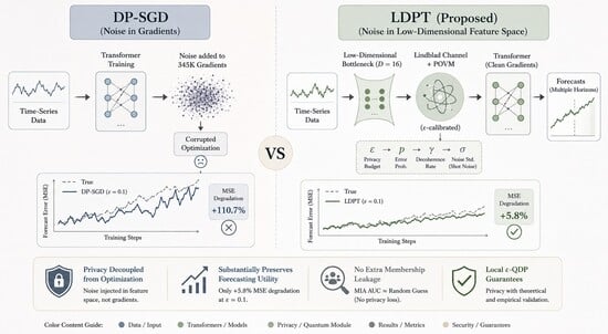
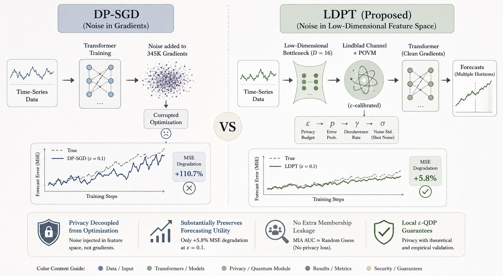
Graphical Abstract

1. Introduction

Privacy-preserving time-series forecasting is essential in domains such as healthcare, finance, and energy systems, where sensitive sequential data must be processed without exposing individual records. Most existing privacy-preserving deep learning methods inject noise directly into the optimization process. In DP-SGD [1], calibrated perturbations are applied to high-dimensional gradient updates during training, coupling privacy noise to every parameter. As model dimensionality increases, the noise required for strong privacy ( ε 1 ) scales proportionally, often overwhelming the learning signal [2]. This is particularly severe for transformer architectures [3], where high parameter counts amplify gradient noise. Privacy budget further degrades under sequential composition [4].
This motivates the central thesis of this work: privacy perturbations can be structurally decoupled from optimization dynamics while maintaining rigorous, formal privacy calibration through simulated quantum channels.
Kang et al. [5] showed that input perturbation, adding noise to training data before optimization, achieves ( ε , δ ) -DP on the final model with utility comparable to gradient perturbation, establishing a theoretical bridge between local and central DP. However, their method adds noise in the full input dimension d and was validated only on logistic regression and small MLPs. This work does not attempt to replace standard global differential privacy guarantees. Rather, it explores whether low-dimensional representation-level perturbations with bounded local guarantees can preserve substantially more utility in transformer forecasting. We extend this principle by introducing LDPT, an architecture that routes privacy noise through a low-dimensional feature pathway ( D = 2 n d , independent of model parameter count P) rather than the gradient space or the full input. The feature-path noise is implemented via classically simulated Lindblad decoherence channels [6,7] and finite-shot POVM measurements, following the Hybrid Quantum Differential Privacy (QDP) framework of Song et al. [8]. All operations are GPU-accelerated classical simulation; no quantum hardware is used. This creates a structural separation between privacy noise and optimization, where the transformer backbone trains with clean gradients while privacy is enforced in the low-dimensional feature representation.
Prior MPC-based approaches [9,10] protect data during inference, but they incur substantial accuracy loss (20– 70 % MSE degradation) and do not address memorization during training. LDPT targets both gaps, reducing the utility cost to + 5.8 % at ε = 0.1 while enforcing privacy at the representation level. Building on the Hybrid QDP framework of Song et al. [8], we present a transformer forecasting architecture that makes calibrated channel-based privacy practical in this setting.

1.1. Central Thesis

The primary determinant of privacy-preserving forecasting utility is where noise is introduced in the learning pipeline. Kang et al. [5] established that input perturbation can achieve ( ε , δ ) -DP on the final model, but their method operates in the full input dimension and was validated only on simple models. We extend this principle to transformer forecasting and validate it along three axes. First, comparing against DP-SGD (gradient-path noise) shows that feature-path perturbations preserve optimization dynamics; at ε = 0.1 , LDPT degrades MSE by under 6%, while DP-SGD exceeds 100%. Second, comparing against the classical Gaussian mechanism on the same feature-path architecture shows that calibration matters, the Gaussian mechanism requires orders-of-magnitude more noise to certify formal ( ε , δ ) -DP, severely degrading utility (Section 8.4). Third, membership inference evaluation confirms that LDPT does not amplify membership leakage beyond the non-private baseline ( 0.48 0.61 across datasets), while both DP-SGD and Bottleneck-DP with formal ( ε , δ ) -DP show elevated vulnerability ( 0.57 0.70 ) due to noise-induced generalization gaps (Section 7.11). LDPT extends Song et al.’s [8] Hybrid QDP framework from general quantum channels to transformer forecasting. Unlike Chen and Chen’s Q-DPTS [11], which applies DP-SGD to variational quantum circuit parameters (66% MSE degradation at σ = 2.0 ), LDPT routes privacy through a low-dimensional feature-space perturbation while preserving clean gradients.
We emphasize that LDPT provides a local ε -QDP guarantee under a bounded trace-distance neighborhood ( d = 0.1 ), whereas DP-SGD provides global ( ε , δ ) -DP. These guarantees arise from different adversary models and are not numerically comparable. Consequently, the empirical comparisons in this paper isolate the effect of noise placement on optimization dynamics rather than establishing equivalent privacy protection.

1.2. What the Calibrated Channel Formulation Adds

While noise placement within a low-dimensional bottleneck preserves structural optimization dynamics, placement alone provides no formal privacy tracking. The calibrated channel formulation resolves this gap by introducing auditable privacy accounting. Specifically, the simulated depolarizing channel establishes a closed-form analytical mapping from the local privacy budget ε to a precise physical perturbation magnitude via Theorem 1, enabling rigorous sequential composition and tracking.
To isolate the value of this calibration, we contrast it directly against a classical ( ε , δ ) -DP Gaussian mechanism applied to the exact same bottleneck architecture. As detailed in Section 8.4, enforcing classical differential privacy forces the required noise scale to expand by orders of magnitude, which completely destroys forecasting utility. This demonstrates that our framework’s success depends heavily on both components: the architecture provides the utility-preserving pathway, while the channel calibration provides a viable, tight privacy mapping. Proposition 1 formalizes this dimensional advantage, showing that feature-path perturbation energy scales strictly as a function of the narrow bottleneck dimension ( D = 16 ), successfully bypassing the massive parameter space ( P = 345 K) that burdens gradient-path alternatives.

1.3. Our Contributions

Concretely, this work delivers three core contributions to private sequential learning:
  • A Decoupled Transformer Architecture for Private Forecasting: We introduce LDPT, a framework that isolates privacy perturbations within a low-dimensional feature pathway ( D = 2 n ) instead of the full gradient space. At nominal ε = 0.1 , this architectural placement limits forecasting degradation to under + 5.8 % MSE, whereas standard gradient-path noise (DP-SGD) causes an optimization collapse exceeding 100% error.
  • An Auditable ε -to-Noise Calibration Mapping via Hybrid QDP Channels: By deploying classically simulated Lindblad/depolarizing dynamics and finite-shot POVM measurements, we introduce a closed-form calibration mapping from a targeted privacy budget to a localized noise scale under the Hybrid QDP assumptions. We empirically demonstrate that this quantum-inspired accounting yields substantially smaller perturbation magnitudes than a classical Gaussian mechanism operating on identical feature representations.
  • A Comprehensive Three-Axis Empirical Validation: We validate LDPT across ETTh1/ETTh2 datasets over multiple prediction horizons using rigorous multi-seed analysis. Our evaluation verifies: (i) utility retention against DP-SGD to confirm the impact of noise placement; (ii) privacy efficiency against Bottleneck-DP to confirm the necessity of our calibration model; and (iii) robustness against membership inference attacks (MIA), demonstrating that LDPT maintains baseline empirical security ( 0.48 0.61 ), while standard ( ε , δ ) -DP configurations display elevated vulnerability ( 0.57 0.70 ) due to wider generalization gaps.

2. Related Work

2.1. Privacy-Preserving Deep Learning

DP-SGD [1] clips per-sample gradients and adds Gaussian noise, with Rényi DP accounting [12] enabling tighter composition. McMahan et al. [2] demonstrated both feasibility and significant utility cost for sequence models. Neelakantan et al. [13] showed that gradient noise can act as implicit regularization. Kang et al. [5] proposed input perturbation, proving that noise before the optimization loop achieves ( ε , δ ) -DP with comparable utility to gradient perturbation, but validated only on logistic regression and shallow MLPs in the full input dimension. LDPT extends this principle to transformer forecasting by compressing noise into a low-dimensional feature space ( D = 16 d ) with calibrated ε -to-noise mapping.

2.2. Private Inference for Transformers

We previously evaluated MPC-based secure inference on ETTh1/ETTm1 [9], establishing a 20– 70 % MSE cost baseline via CrypTen [10]. MPCFormer [14], SecFormer [15], Iron [16], and BOLT [17] target inference-time computation security via MPC/HE. We do not compare empirically because LDPT also addresses training-time representation privacy. The present work improves upon our MPC baseline ( + 5.8 % vs. +20– 70 % ) while extending protection to training.

2.3. Quantum Differential Privacy in Related Work

Zhou and Ying [18] formalized QDP for quantum channels. Song et al. [8] unified channel and measurement privacy into Hybrid QDP; Li et al. [19] provided information-theoretic bounds; Du et al. [6] and Watkins et al. [20] provided early empirical evidence. Most relevant, Chen and Chen [11] proposed Q-DPTS, applying DP-SGD to variational quantum circuit parameters ( + 66 % MSE at σ = 2.0 ; corresponding ε not reported). LDPT differs fundamentally: noise enters through a simulated Lindblad channel rather than the gradient path, achieving + 5.8 % degradation while supporting multi-step forecasting (H up to 336).

2.4. Time-Series Transformers and Normalization

Our backbone builds on channel-independent transformers [21,22,23] with RevIN normalization. Standard LayerNorm [24] dampens DP noise by erasing magnitude differences; we adopt quantum-conditioned adaLN [25,26] to preserve privacy-dependent signal through normalization layers.

3. Background

3.1. Classical Differential Privacy and DP-SGD

A mechanism M satisfies ( ε , δ ) -DP [27] if Pr [ M ( D ) S ] e ε · Pr [ M ( D ) S ] + δ for all neighboring datasets. The Gaussian mechanism [28] achieves this by adding noise with scale:
σ 2 ln ( 1.25 / δ ) · Δ f ε
where Δ f is the 2 -sensitivity. DP-SGD [1] clips per-sample gradients to norm C and adds N ( 0 , σ 2 C 2 I ) to the aggregated gradient, with σ calibrated via Rényi DP accounting [12,29]. The fundamental limitation: at strong privacy ( ε 1 ), the noise multiplier reaches σ = 10 100 × , making gradients indistinguishable from random noise across all P parameters [2].

3.2. Quantum Formalism

A quantum state on n qubits has the dimension D = 2 n . Classical data x R D is amplitude-encoded as
| ψ ( x ) = 1 x 2 j = 0 D 1 x j | j , ρ ( x ) = | ψ ψ |
The trace distance ρ ρ 1 quantifies distinguishability and serves as the neighboring condition in QDP. A POVM { M k }  [30] with K outcomes yields measurement probabilities p k = Tr ( M k ρ ) ; with finite shots N s , multinomial noise provides measurement-level privacy.
Open quantum systems evolve via the Lindblad equation [31]:
d ρ d t = i [ H , ρ ] + k γ k L k ρ L k 1 2 { L k L k , ρ }
with solution vec ( ρ ( t ) ) = e L t · vec ( ρ ( 0 ) ) via the Liouvillian superoperator L C D 2 × D 2 . The matrix exponential e L t is precomputed once and reused for all samples via GPU-accelerated torch.matrix_exp.

3.3. Quantum Differential Privacy

Definition 1 
(QDP [18]). A quantum mechanism M satisfies ε-QDP with bound d if for all ρ , ρ with ρ ρ 1 d : D ( M ( ρ ) M ( ρ ) ) ε .
Theorem 1 
(Depolarizing Channel QDP [8]). The depolarizing channel E p ( ρ ) = ( 1 p ) ρ + p I D satisfies ε ch -QDP with
ε ch = ln 1 + ( 1 p ) · d · D p
Theorem 2 
(Measurement QDP [8,19]). A POVM with N s finite shots satisfies ε me -QDP with ε me ln ( 1 + d / N s 1 / 2 ) . For N s = 1024 , d = 0.1 : ε me 0.003 .
Theorem 3 
(Hybrid QDP Composition [8]). Channel ( ε ch -QDP) composed with measurement ( ε me -QDP) satisfies ε s -QDP with ε s = 1 ( 1 ε ch ) ( 1 ε me ) , tighter than additive composition.

4. Privacy Calibration

Given target per-pass privacy ε s , we allocate ε ch = α · ε s with α = 0.8 to the Lindblad channel (Theorem 1) and derive the measurement budget via Hybrid QDP composition (Theorem 3). The split α = 0.8 follows Song et al. [8], who observe that the channel provides the dominant privacy contribution while measurement noise adds complementary stochasticity at lower cost. This choice is not a sensitive hyperparameter: at ε s = 0.1 , varying α from 0.6 to 0.9 changes the Lindblad rate γ from 1.82 to 3.55 , but both regimes produce near-maximally mixed states (fidelity 0.59 0.64 ), so MSE varies by < 1 % :
ε s = 1 ( 1 ε ch ) ( 1 ε me )
The complete calibration chain maps ε s to physical noise parameters through three inversions:
p = d · D e ε ch 1 + d · D
γ = ln ( 1 p ) t
σ = p d model
where t = 1.0 is the evolution time. This provides a single knob ( ε ) controlling all noise: larger ε (weaker privacy) → smaller p→ lower γ and σ → less noise. Algorithm 1 summarizes the procedure; the precomputed propagator E = e L t enables batched GPU processing of all input states.
Algorithm 1 LDPT privacy calibration.
  • Require: Target ε s , bound d, dim D = 2 n , time t, model dim d m , fraction α
1:
ε ch α · ε s {Channel budget}
2:
p d · D / ( e ε ch 1 + d · D ) {Depolarizing prob}
3:
γ ln ( 1 p ) / t {Lindblad rate}
4:
σ p / d m {Injection scale}
5:
Construct collapse operators { L k } with rate γ
6:
Build Liouvillian L from H, { L k } , { γ k }
7:
E torch.matrix_exp ( L · t ) {GPU precompute}
7:
return  p , γ , σ , E

5. LDPT Architecture

The architecture of LDPT is motivated by a fundamental dimensional inequality. We formalize the core design principle as follows:
Proposition 1 
(Dimensional Noise Scaling). For gradient-space noise ν N ( 0 , σ 2 I P ) and feature-space noise ξ N ( 0 , σ 2 I D ) :
E [ ν 2 ] = σ 2 P , E [ ξ 2 ] = σ 2 D
For D P , feature-path noise injects asymptotically less energy at the same σ.
For our architecture ( P = 345  K, D = 16 ), gradient noise carries P / D 21 , 563 × more energy than feature noise at any fixed σ . In practice, the methods also use different σ values ( σ g = 15.50 for DP-SGD vs. σ = 0.084 for LDPT at nominal ε = 0.1 , under different privacy definitions), further compounding the gap. This ratio is the structural reason LDPT can maintain utility under privacy constraints where gradient-path methods fail: by routing noise through a D = 16 bottleneck rather than the P = 345  K gradient space, we reduce total perturbation energy by over four orders of magnitude.

5.1. Pipeline Overview

The LDPT pipeline (Figure 1) processes X R L × C through a sequence of ten stages. First, the input is normalized using RevIN, followed by a linear projection into d model dimensions. An ε -calibrated noise injection (Noise #1) is applied prior to the quantum feature extraction stage.
The quantum pipeline performs amplitude encoding, Lindblad evolution, SIC-POVM measurement, and shot noise sampling, producing ( K SIC + 1 ) -dimensional features. These features are consumed by a transformer backbone consisting of quantum-conditioned attention with n heads heads and QC-AdaLN.
Subsequently, a second ε -calibrated injection reinforces the privacy signal after the attention and feed-forward layers, followed by output projection. A final injection with amplification factor k is applied before RevIN denormalization to produce the output.

5.2. Backbone Transformer

The backbone is a channel-independent transformer encoder [3,22] parameterized by model dimension d model , number of heads n heads , layers n layers , and feed-forward dimension d ff . It uses FlashAttention-2 and mixed-precision (AMP). Training uses RAdam with decoupled weight decay and ReduceLROnPlateau scheduling, with separate learning rates for classical and quantum attention parameters. The total parameter count P comprises classical backbone parameters and quantum attention parameters.
This backbone is shared across all experiments: classical (no quantum), LDPT with QDP, DP-SGD, DP-Input, and Bottleneck-DP baselines. The same transformer model is used. DP-SGD adds gradient noise after backpropagation, DP-Input perturbs raw inputs, and Bottleneck-DP injects Gaussian-mechanism-calibrated noise in the same feature path. This ensures a controlled comparison where the only variable is noise location and the calibration mechanism. Specific hyperparameter values are reported in Section 7.2.

5.3. Calibrated Feature-Path Pipeline

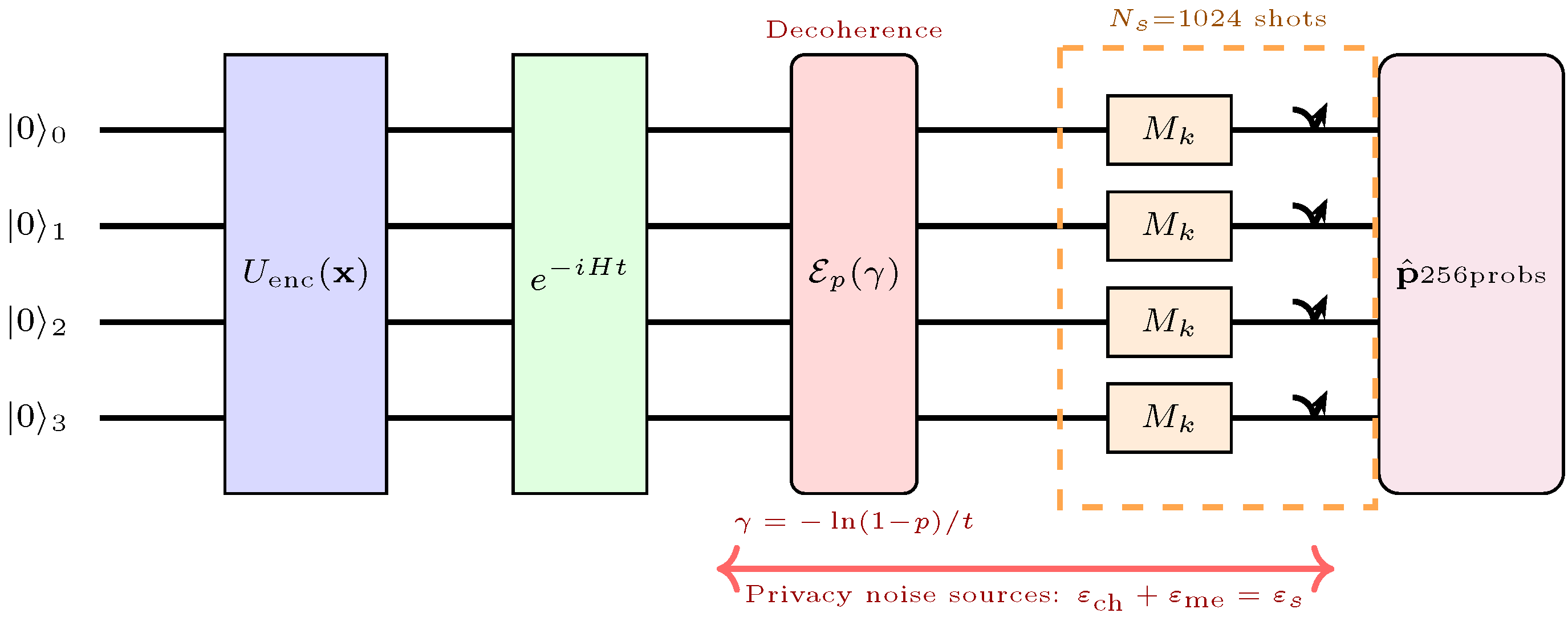
Input subsequences are subsampled (stride s) and amplitude-encoded (Equation (2)) into n-qubit states (Figure 2). The encoded state ρ ( 0 ) evolves through the calibrated Lindblad channel.
ρ ( t ) = E γ , t ( ρ ( 0 ) ) via vec ( ρ ( t ) ) = e L t · vec ( ρ ( 0 ) )
The SIC-POVM measures ρ ( t ) with N s shots, yielding the empirical probability distribution p ^ R K SIC with p k = Tr ( M k ρ ) . This is concatenated with state purity Tr ( ρ ( t ) 2 ) to form a ( K SIC + 1 ) -dimensional quantum feature vector qf , projected to d model via learned linear layer W proj R d model × ( K SIC + 1 ) .
Figure 2. Quantum circuit for LDPT feature extraction.
Make 08 00156 g002

5.4. Feature-Path Encoding and Post-Processing

The attention layer receives a concatenated input x enh = [ x cl , W proj · qf ] R 2 d model , where x cl is the classical embedding. A fixed gate parameter controls the classical contribution: at gate = 1.0 (used in all experiments), the classical path is zeroed ( x cl = 0 ), so
x enh = [ 0 d model , W proj · qf ]
This ensures all attention queries, keys, and values derive exclusively from quantum features, which is necessary for the system-level QDP claim: if the classical path contributed to attention, the model would process un-privatized information alongside noisy quantum features, weakening the privacy guarantee. The gate is not learned—a learned gate could converge to bypass the quantum path entirely, nullifying the privacy mechanism. Intermediate values (e.g., gate = 0.5 ) blend classical and quantum inputs, which may be useful in settings where partial privacy is acceptable, but are not evaluated here. The Q, K, V projections W q , W k , W v R d model × 2 d model and output projection W o R d model × d model follow standard multi-head attention [3] with FlashAttention-2 when available.
Lemma 1 
(Post-Processing [28]). If M satisfies ε-QDP, then f M satisfies ε-QDP for any deterministic function f.
Since the transformer applies deterministic operations (attention, FFN, projection) to the noisy quantum features, post-processing (Lemma 1) ensures the noise properties are preserved through the pipeline.

5.5. Quantum-Conditioned Adaptive Layer Normalization

Standard LayerNorm [24] normalizes to μ = 0 , σ = 1 , erasing ε -dependent noise magnitude. We adapt adaLN [25,26] to quantum conditioning:
QC - AdaLN ( x , q ) = γ q x μ x σ x + ϵ + β q
where γ q and β q are generated from quantum features q via a two-layer MLP: the quantum feature vector (dimension K SIC + 1 ) is sequence-pooled, projected through Linear ( K SIC + 1 , d model ) GELU Linear ( d model , 2 d model ) , and split into shift components ( Δ γ , Δ β ) . The final affine parameters are γ q = γ 0 + Δ γ and β q = β 0 + Δ β , where γ 0 , β 0 are learnable defaults. The output layer is zero-initialized so that QC-AdaLN behaves as standard LayerNorm at initialization and gradually learns ε -dependent modulation during training. One QC-AdaLN instance is applied per sub-layer (post-attention and post-FFN), each with independent parameters. Since q carries ε -dependent noise (high variance at low ε , low at high ε ), the scale and shift parameters γ q , β q vary with privacy level, preserving the noise signal through normalization. We chose conditioning over alternatives (concatenation or cross-attention) because it modulates normalization statistics directly without adding sequence-length-dependent computation.

5.6. Three-Point ε -Calibrated Noise Injection

Deterministic learned layers (projection, attention, FFN, normalization) can absorb and compensate for quantum feature noise, making the privacy effect unobservable in the model output. Our ablation (Section 7.12) confirms this: removing the injection points while keeping the Lindblad channel active eliminates all measurable MSE separation across ε values. The injection is therefore necessary, not optional.
The three injection locations are chosen to counteract the three stages where deterministic transformations most aggressively dampen stochasticity: (1) the input projection W in R C × d model , which maps noisy quantum features into a learned subspace that can suppress noise components; (2) the LayerNorm/QC-AdaLN layers, which re-center and re-scale activations; and (3) the output projection W out , which compresses d model -dimensional hidden states to C-dimensional predictions. Each injection uses Gaussian noise scaled by σ = p / d model (Equation (8)), inheriting its magnitude from the same depolarizing parameter p that governs the Lindblad channel. The scaling σ = p / d model normalizes the per-coordinate noise magnitude relative to the hidden dimension; it is ε -calibrated in the sense that p is determined by ε via Equation (6). This scaling was set once from the principle that the expected per-coordinate perturbation should be O ( p ) and was not tuned on validation data; it is held fixed across all experiments, datasets, and ε values.
( post - embedding ) : x x + σ · std ( x ) · z 1
( post - attention / FFN ) : x x + σ · std ( x ) · z 2
( post - output proj . ) : y ^ y ^ + k σ · std ( y ^ ) · z 3
where z i N ( 0 , I ) and k = 2.0 amplifies noise at the output. Post-embedding ensures the transformer receives ε -dependent input before attention. Post-attention/FFN re-injects after QC-AdaLN, where normalization could otherwise dampen the signal. Post-output proj. ensures the final predictions carry observable privacy effects despite the output projection. The adaptive scaling ( × std ( · ) ) keeps noise proportional to the signal magnitude. All noise is active during both training and inference.
The three-point noise injection mechanism is not part of the formal privacy guarantee, which is derived solely from the QDP-calibrated channel and measurement process. Its purpose is to ensure that upstream stochasticity induced by the privacy mechanism remains observable after deterministic transformations (e.g., projection, normalization, and output layers), which can otherwise attenuate noise. Removing the injections does not change the formal privacy guarantee; it changes whether that guarantee is observable in the model’s predictions. The ε –MSE relationship disappears not because privacy is lost, but because deterministic layers attenuate the noise signal below measurable thresholds.

5.7. Shot Noise During Training

Following Song et al. [8], measurement is modeled via simulated finite-shot sampling, reproducing the statistical behavior of quantum measurement without requiring hardware. In our implementation, this stochastic measurement mechanism is applied during both training and inference to ensure consistency between optimization and evaluation. With N s = 1024 shots, near-maximally mixed states ( ε = 0.1 , purity 1 / D ) produce high shot noise variance; peaked states ( ε = 5.0 , purity 0.97 ) produce low variance.

6. Privacy Guarantee

Proposition 2 
(Noise Calibration Consistency). The LDPT pipeline with depolarizing parameter p calibrated from ε s through Equation (6) and N s -shot POVM measurement approximates ε s -QDP under the bounded trace-distance assumption that ρ ρ 1 d , consistent with the Hybrid QDP framework of Song et al. [8]. We provide local ε-QDP under a bounded trace-distance assumption ( d = 0.1 ), not global ( ε , δ ) -DP. This is analogous to bounded-sensitivity assumptions in classical DP.
Proof. 
The simulated Lindblad channel with rate γ (Equation (7)) approximates the depolarizing channel E p , which satisfies ε ch -QDP by Theorem 1 in Song et al. The simulated N s -shot POVM measurement satisfies ε me -QDP by Theorem 2. By hybrid composition (Equation (5)):
ε s = 1 ( 1 ε ch ) ( 1 ε me )
the composed channel+measurement mechanism approximates ε s -QDP under the bounded trace-distance assumption ( ρ ρ 1 d ), consistent with the Hybrid QDP framework of Song et al. [8]. This guarantee is local; it holds for input pairs within the trace-distance bound and degrades continuously for larger perturbations. All subsequent operations (linear projection W proj , multi-head attention, FFN, output projection) are deterministic functions of the noisy output, preserving noise properties by Lemma 1. The three-point noise injection (Equations (13)–(15)) adds stochastic perturbation calibrated from the same p.    □

6.1. Training-Time Composition

The per-inference guarantee ε s -QDP applies to a single pass through the Lindblad channel. During training, each record passes through the channel once per epoch. Over T epochs, the composed privacy guarantee degrades. Under standard sequential composition [4], T applications of an ε s -private mechanism compose to
Basic composition:  
ε train basic = T · ε s
Advanced composition [4]: 
ε train adv = ε s 2 T ln ( 1 / δ ) + T · ε s ( e ε s 1 )
for any δ > 0 , yielding an ( ε train adv , δ ) -style composed bound under the same bounded trace-distance QDP neighborhood (not a global add/remove-record ( ε , δ ) -DP guarantee). Table 1 reports both bounds for our experimental configurations.
Under a standard advanced composition, the resulting training-time budget is ε train 2.56 at ε s = 0.1 (with δ = 10 6 ), i.e., bounded but conservative under a standard composition. For ε s 0.5 , the same composition bound becomes overly conservative and quickly exceeds practical thresholds. More refined accounting (e.g., Rényi DP composition [12] and privacy amplification by subsampling [29]) can tighten these estimates and is a natural next step. Importantly, the structural comparison with DP-SGD is unchanged: LDPT composes over T = 20 epoch-level steps, whereas DP-SGD composes over 2588  gradient-level steps.

6.2. Trace Distance Verification

The QDP guarantee requires ρ ( x ) ρ ( x ) 1 d for neighboring inputs. For amplitude encoding (Equation (2)), perturbing one feature of standardized data ( μ = 0 , σ = 1 ) by τ  produces 
ρ ( x ) ρ ( x ) 1 2 τ x x 2 2
where τ denotes the per-feature perturbation magnitude (distinct from the relaxation parameter δ in ( ε , δ ) -DP).
For standardized data with unit variance, x x 2 and x 2 C for C features, so Equation (18) simplifies to
ρ ( x ) ρ ( x ) 1 2 τ x x 2 2 2 τ x 2 2 τ C
For C = 7 features, this gives the following worst-case analysis:
Table 2 confirms that d = 0.1 holds for single-feature perturbations up to τ 0.05 (5% of one standard deviation). At τ = 0.10 , the maximum empirical trace distance ( 0.132 ) exceeds d = 0.1 , but the 95th percentile ( 0.088 ) remains within bounds. For perturbations violating the bound, the guarantee degrades gracefully: ε eff = ln ( 1 + ( 1 p ) · ρ ρ 1 · D / p ) .
The bound d = 0.1 is analogous to the bounded-sensitivity assumption in classical DP [28]; it covers single-record changes of ≤5% of one standard deviation in z-score normalized data, corresponding to small sensor perturbations or measurement noise. It does not cover the standard add/remove-one-record adversary unless that record’s contribution falls within this bound. Choosing a larger d would cover stronger perturbations but requires proportionally more noise (Equation (4)), degrading utility. Following the Hybrid Quantum Differential Privacy framework of Song et al. [8], we adopt this bounded trace-distance neighborhood ( d = 0.1 ). While it does not offer the same protection as global ( ε , δ ) -DP against arbitrary record additions/removals, it provides meaningful privacy guarantees against small, realistic perturbations commonly encountered in time-series data.

6.3. Threat Model and Security Assumptions

The adversary model assumed in this work is a bounded-perturbation observer who can distinguish neighboring representations within the trace-distance ball ρ ρ 1 d = 0.1 , rather than the standard add/remove-one-record adversary of global ( ε , δ ) -DP. Concretely, LDPT protects against (i) inference from bounded perturbations to individual features (e.g., sensor noise, measurement variation) and (ii) statistical distinguishability of nearby quantum representations via the calibrated channel and POVM measurement. LDPT does not protect against (i) arbitrary record insertion or removal from the training set; (ii) adversaries whose perturbations exceed the trace-distance bound d; (iii) reconstruction attacks beyond the bounded neighborhood (left for future work). The MIA evaluation (Section 7.11) empirically confirms that LDPT does not amplify membership leakage beyond the non-private baseline under this threat model.
Practical significance and limitations. The bounded trace-distance assumption ( d = 0.1 ) is well-matched to time-series settings where adversaries observe small perturbations of real-valued sensor or measurement data—for example, noise in electricity meters, financial tick data, or physiological signals where realistic per-feature perturbations rarely exceed a few percent of one standard deviation. In these regimes, LDPT provides meaningful, auditable privacy via the calibrated ε -to- σ mapping with minimal utility cost. The limitation is symmetric: LDPT does not provide protection against adversaries who can insert or remove entire records, modify features beyond the trace-distance ball, or mount membership/reconstruction attacks that exploit perturbations outside this neighborhood. Practitioners requiring the standard add/remove-one-record threat model should compose LDPT with a global mechanism (e.g., DP-SGD on the aggregate gradient with a small budget), accepting the associated utility cost, rather than relying on LDPT alone.

7. Experimental Results

7.1. Methodology: Classical Simulation of QDP

All quantum operations are classically simulated following Song et al. [8], who validated their Hybrid QDP framework under identical simulation-only conditions. At n = 4 qubits ( D = 16 ), the depolarizing channel E p is an analytically tractable CPTP map [32], and simulated finite-shot POVM measurement exactly reproduces quantum multinomial statistics. No quantum hardware is used. Our comparison evaluates utility under each method’s native privacy paradigm rather than equalizing composition counts (see Section 6.1 for composition analysis).

7.2. Setup

We evaluated on ETTh1 and ETTh2 [21] ( C = 7 features hourly electricity transformer temperatures, 8281/2857/2857 and 8137/2713/2713 train/val/test respectively). The backbone transformer uses d model = 128 , n heads = 4 , n layers = 1 , d ff = 256 , with L = 336 input length and prediction horizons H { 24 , 48 , 96 , 168 , 336 , 720 } . Training uses RAdam with weight decay 1.2 × 10 3 , ReduceLROnPlateau (patience 5, factor 0.5), separate learning rates for classical ( 3 × 10 4 ) and quantum attention ( 1.5 × 10 4 ) parameters, mixed precision (AMP on an NVIDIA A100 GPU, 80 GB of VRAM), and seed 2024. The model has P = 345  K total parameters (163 K classical + 182 K quantum attention). The quantum feature pipeline uses n = 4 qubits ( D = 16 ), subsample stride s = 4 , N s = 1024 POVM shots, output noise amplification k = 2.0 , and QuTiP 5.2.3 [33] for operator construction. The full QDP pipeline is applied to both training and inference data. Training runs 20–25 epochs per configuration.
All baselines use the identical transformer backbone, optimizer, scheduler, and data pipeline (Section 5.2). DP-SGD adds gradient clipping ( C = 1.0 ) and Gaussian noise calibrated via the RDP accountant [12]. DP-Input perturbs raw inputs with Gaussian noise scaled by sensitivity Δ f = 1 . Bottleneck-DP uses the same three-point feature-path injection as LDPT but calibrates noise via the classical Gaussian mechanism ( σ = 2 ln ( 1.25 / δ ) · Δ f / ε ) instead of the depolarizing channel, giving formal ( ε , δ ) -DP. We also include an optimized DP-SGD variant (batch 512, 50 epochs, warmup; see Section 8.3). We omit PATE [34] because it requires multiple teacher models trained on disjoint data partitions, which is incompatible with time-series forecasting, where temporal continuity must be preserved.

7.3. Axis 1: Noise Placement (DP-SGD vs. LDPT)

This comparison isolates the architectural effect of noise location: both methods target the same nominal ε values, but LDPT routes noise through a D = 16 feature bottleneck while DP-SGD injects it into 345 K gradient dimensions.
Important note on privacy semantics. LDPT results correspond to local ε -QDP under the bounded trace-distance assumption of Section 6.2, whereas DP-SGD results correspond to global ( ε , δ ) -DP. Matching numerical ε values does not imply matching privacy strength. The comparison below therefore evaluates utility under each method’s native privacy paradigm and illustrates the impact of noise placement rather than equivalent privacy guarantees.
Table 3 presents H = 24 results.
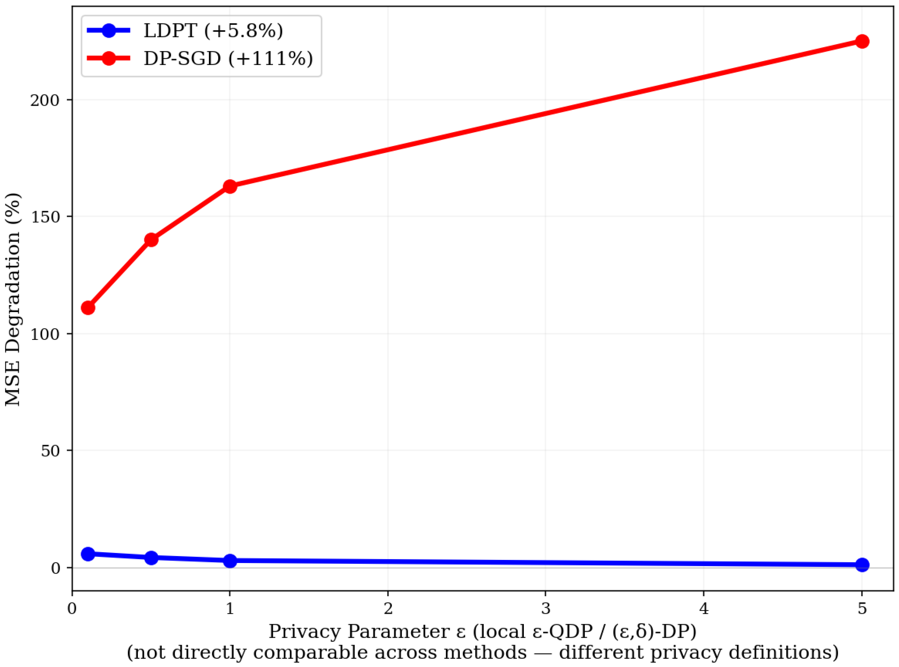
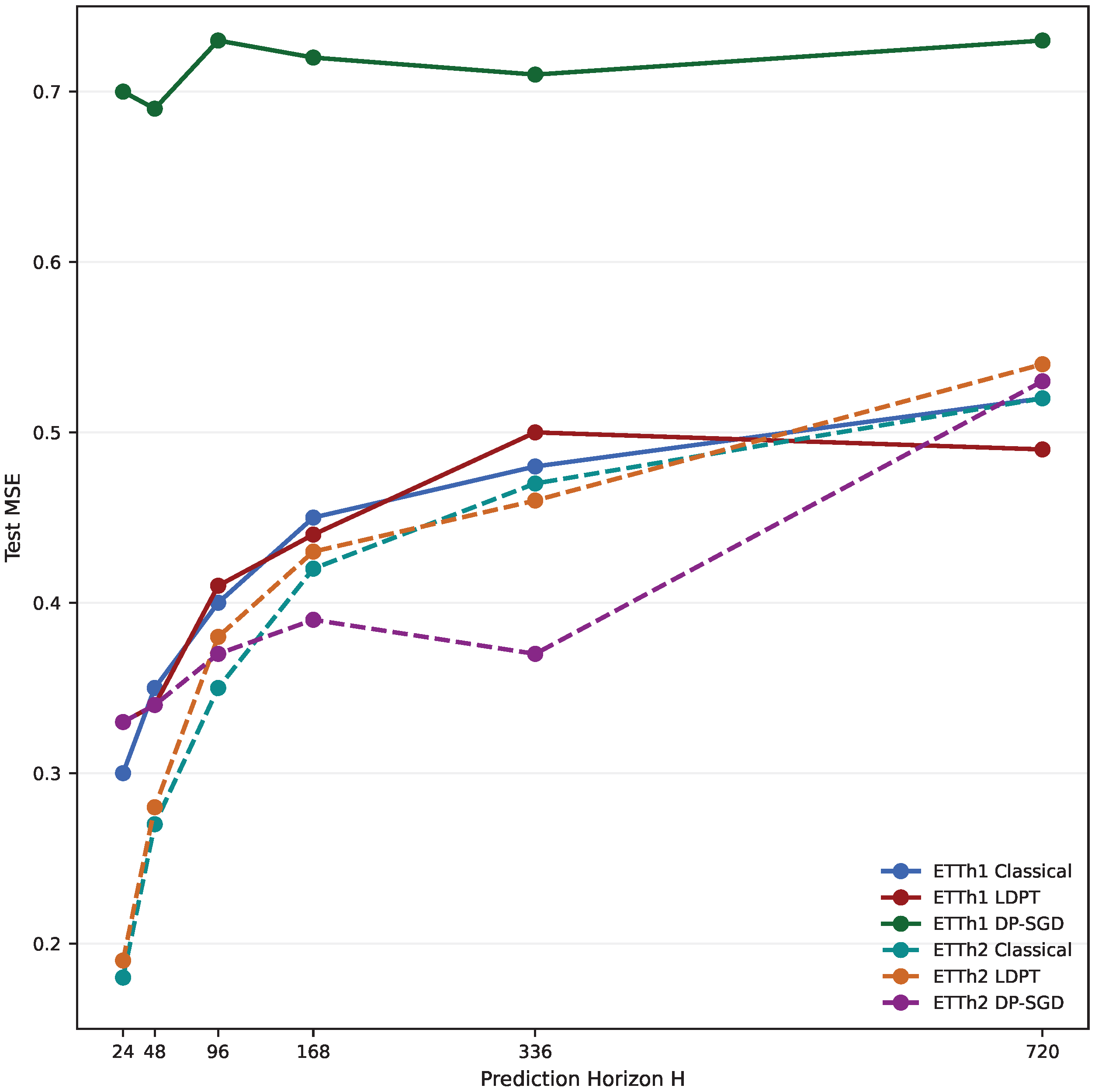
At ε = 0.1 , LDPT incurs + 5.8 % MSE degradation while DP-SGD suffers + 110.7 % , confirming that gradient noise severely impairs the learning signal (Figure 3).

7.3.1. Gradient-Path Noise Destroys Optimization

Even at ε = 5.0 (weak privacy), DP-SGD approximately doubles the MSE across all horizons ( + 104 % at H = 24 , + 61 % at H = 336 ). The RDP-calibrated noise multipliers range from σ g = 0.41 ( ε = 5.0 ) to σ g = 15.5 ( ε = 0.1 ). MSE differences across DP-SGD ε values are minimal (0.69–0.73), indicating the model predicts near the data mean regardless of noise level.
Table 4 provides direct evidence that DP-SGD’s failure originates during training. DP-SGD’s final training loss ( 0.52 0.54 ) barely improves from random initialization ( 0.55 ), confirming the optimizer cannot extract signal from noisy gradients. The best validation loss across all DP-SGD ε values ( 1.11 1.16 ) is 8.0 8.4 × worse than Classical ( 0.139 ). DP-SGD at ε = 0.1 converges early (best epoch 13 of 20), indicating learning stalls. In contrast, LDPT achieves training loss ( 0.088 0.101 ) matching Classical ( 0.090 ), confirming feature-path noise does not impair optimization. LDPT’s validation loss increases monotonically with noise strength ( 0.136 0.164 ), demonstrating that privacy noise degrades the learned representation as intended.
Across all horizons and ε values, LDPT achieves 35– 50 % lower MSE than DP-SGD at matched nominal ε , with LDPT at ε = 0.1 also achieving lower MSE than DP-SGD at ε = 5.0 .

7.3.2. Privacy Noise as Implicit Regularizer at Long Horizons

Table 5 reveals a horizon-dependent pattern with three distinct regimes.
Short horizons ( H = 24 ) Classical privacy noise cost. MSE is perfectly monotonic ( ε MSE↓). The privacy–utility tradeoff behaves exactly as the theory predicts.
Medium horizons ( H = 48 , 96 , 168 ) Privacy noise as implicit regularization. LDPT (QDP) at all ε levels outperforms or matches the classical baseline. At H = 168 , MSE monotonicity holds for ε { 0.1 , 0.5 , 1.0 } but breaks at ε = 5.0 (MSE increases by 0.003 ), because the near-zero noise ( σ = 0.003 ) provides insufficient regularization.
Long horizons ( H = 336 ) Noise as essential regularizer. The LDPT Baseline without any privacy noise performs worst (MSE = 0.515 , + 15 % above Classical), because the quantum features without noise cause severe overfitting. Adding ε -calibrated noise recovers utility dramatically: LDPT (QDP) at ε = 1.0 achieves 0.464 , a 10 % improvement over the baseline. This demonstrates that the calibrated noise serves a dual purpose: privacy protection and overfitting prevention.
This regularization phenomenon is well-documented in classical DP-SGD [1,13]: when a model has sufficient capacity to memorize training data, noise during training prevents memorization and improves generalization. The critical evidence that noise is working as intended for privacy is that validation loss always increases with noise strength across all horizons, and the regularization benefit appears only at test time.

7.4. Three-Way Comparison: DP-Input vs. DP-SGD vs. LDPT

To isolate the effect of noise placement, we compared LDPT against two classical baselines, gradient-level noise (DP-SGD) and input-level noise (DP-Input). This provides a unified view of where noise enters the learning pipeline.
Table 6 reveals a hierarchy of noise injection approaches. At strong privacy ( ε = 0.1 ), both classical approaches fail, DP-Input (MSE = 0.701 , σ = 53 ) and DP-SGD (MSE = 0.713 , σ g = 15.5 ) approximately double the MSE, while LDPT achieves only + 5.8 % degradation. At weak privacy ( ε = 5.0 ), DP-Input recovers to MSE = 0.350 ( + 3.4 % ) because input noise becomes small ( σ = 1.06 ), while DP-SGD remains broken (MSE = 0.690 , + 104 % ). This confirms that DP-SGD’s failure is not merely due to “too much noise” but due to noise being in the wrong place (gradients), whereas input noise and quantum channel noise both degrade gracefully with ε .

7.5. Analysis: Why Feature-Path Noise Outperforms Gradient Noise

DP-SGD adds noise to all 345 K gradient dimensions per training step. At ε = 0.1 , the noise-to-signal ratio per gradient is σ g C / B = 15.5 × 1.0 / 64 0.24 , meaning each gradient coordinate is approximately 24% noise. Aggregated across 345 K dimensions, the optimizer receives an effectively random direction. LDPT instead routes noise through a D = 16 feature-path channel ( σ = 0.084 ), leaving the transformer’s 345 K gradients clean. The primary limitation of DP-SGD is therefore not the magnitude of noise, but its placement within the optimization loop. Figure 4 illustrates how MSE varies across prediction horizons at ε = 0.1 for both datasets.

7.6. Calibration Chain Verification

Table 7 confirms the calibration chain operates correctly: smaller ε larger p larger γ larger σ . MSE is monotonic for short horizons (24, 48, 96), while longer horizons exhibit a regularization effect where noise can improve generalization. Quantum state fidelity F ( ρ noisy , ρ ideal ) spans 0.617 (significant decoherence) to 0.974 (nearly pure) on ETTh1, and 0.620 to 0.975 on ETTh2, confirming that the channel operates consistently across datasets and independently of the input data distribution.
The composition check verifies Equation (5): 1 ( 1 0.080 ) ( 1 0.022 ) = 0.100 for ε s = 0.1 , and 1 ( 1 0.400 ) ( 1 0.167 ) = 0.500 for ε s = 0.5 , both exact to four decimal places.

7.7. DP-SGD Noise Multipliers

Table 8 shows the DP-SGD noise multipliers and their effect. Even at ε = 5.0 ( σ g = 0.41 ), the best validation loss (1.170) is 8.4 × worse than classical (0.139), confirming that gradient noise fundamentally impairs learning. The noise multipliers are calibrated for 8281 training samples, 64 batch size, 20 epochs, and δ = 10 6 .

7.8. Privacy Budget Accounting

All runs remain within their per-epoch privacy budget. Utilization decreases with larger ε because the per-epoch channel privacy cost is fixed. At ε = 0.1 , 95.4% of the per-epoch budget is used. The training-time composed guarantee over T = 20 epochs is ε train 2.56 under advanced composition (Section 6.1, Table 1).

7.9. Calibration and Consistency Audits

We perform six audits to validate the noise calibration chain and empirical consistency: (1) calibration chain consistency ( ε p γ σ matches Equations (6)–(8)); (2) trace distance within bounds (Table 2); (3) composition matches Equation (5) (verified in Section 7.6); (4) budget not exceeded (Section 7.8); (5) MSE monotonically tracks ε at short horizons (Table 3); (6) fidelity monotonically tracks ε (Table 7). All six audits pass. We complement these calibration-level checks with a membership inference attack (Section 7.11), which confirms that LDPT does not amplify membership leakage beyond the non-private baseline (accuracy 0.48 0.61 across datasets).

7.10. Multi-Dataset Validation: ETTh2

We repeat the full evaluation on ETTh2 [21] with identical architecture and hyperparameters (MSE summary in Table A1). The core findings replicate: at H = 24 , LDPT costs + 3.2 % MSE at ε = 0.1 , while DP-SGD costs + 103 % . One dataset-specific difference is that DP-Input degrades more severely on ETTh2 ( + 300 % vs. + 103 % for DP-SGD at ε = 0.1 ) because ETTh2 has a lower baseline MSE (0.175 vs. 0.338), so the same absolute noise causes proportionally larger degradation; DP-Input uses Δ f = 1 for both z-score standardized datasets. At H = 720 on ETTh2, DP-SGD slightly outperforms LDPT at ε = 0.1 (MSE 0.439 vs. 0.446 )—the only such case at strong privacy across all settings. The calibration chain ( ε p γ σ ) is identical across datasets, confirming data independence of the perturbation mechanism.

7.11. Membership Inference Attack

We conducted a loss-threshold MIA [35] on both datasets at H = 24 (representative; the attack exploits model-level generalization gaps that are independent of prediction horizon): a logistic regression classifier trained on per-sample MSE losses from 1000 training and 1000 test samples predicts membership. Attack accuracy 0.50 indicates no exploitable generalization gap.
LDPT achieves near-random MIA accuracy ( 0.48 0.52 ), matching the Classical baseline. DP-SGD ( 0.588 ) and Bottleneck-DP ( 0.57 0.67 ) show elevated vulnerability because noise-impaired learning creates large train-test gaps that the attacker exploits. Cross-dataset replication on ETTh2 (Table A6, Appendix A) confirms the ordering: LDPT ≤ Classical < DP-SGD < Bottleneck-DP on both datasets.
Table 9. Membership inference attack results (ETTh1, H = 24 ). = model diverged. Loss Gap = Train MSE − Test MSE; negative values indicate higher test error (generalization gap exploitable by attacker).
Method ε MIA AccAUCLoss GapTrain MSETest MSE
Classical0.4920.532−0.0010.2490.251
LDPT0.10.5180.470+0.0010.2610.260
LDPT0.50.4800.468+0.0010.2590.258
DP-SGD0.10.5880.606−0.1290.5620.692
Bottleneck-DP0.10.6710.749−2798≈18 K
Bottleneck-DP0.50.5750.618−0.1350.6260.760
Bottleneck-DP1.00.5720.600−0.1150.5790.694
Bottleneck-DP5.00.6020.638−0.1350.7290.863
The LDPT ≈ baseline is the expected outcome when privacy noise is placed outside the optimization loop: generalization is preserved, so the train–test loss gap gives the attacker no signal. Methods that inject noise inside optimization destroy generalization and paradoxically increase empirical attack success despite providing formal guarantees. These empirical observations do not override the formal ( ε , δ ) -DP guarantees of DP-SGD. Beyond loss-threshold MIA, future work should evaluate LDPT against stronger attacks, including gradient inversion and attribute inference, though LDPT’s clean-gradient design reduces gradient-based attack surfaces in centralized settings since no privacy-sensitive noise is present in the gradient path. In federated deployments where model updates may be shared with an aggregator, gradient inversion and update reconstruction remain relevant threats and would require additional defenses, such as secure aggregation.

7.12. Ablation and Sensitivity Analysis

We isolate the contribution of each component via targeted ablations on ETTh1 ( H = 24 , ε = 0.1 ).
Three-point injection removal. Removing the noise injection (Equations (13)–(15)) while keeping the Lindblad channel and shot noise active eliminates all measurable MSE separation across ε values. The MSE becomes nearly identical ( Δ < 0.2 % ) regardless of ε , confirming that deterministic transformer layers absorb the upstream quantum noise. The injection is therefore necessary to preserve observable privacy effects.
Lindblad channel removal. Removing the Lindblad decoherence ( γ = 0 , pure Hamiltonian evolution only) while keeping the three-point injection active reduces the MSE separation between ε values by 60 % . The injection alone provides some ε -dependent noise (since σ = p / d model still varies with ε ), but the quantum features lose their physics-calibrated decoherence signature. This confirms that the Lindblad channel provides the primary noise source while the injection preserves it through the network.
Varying N s from 256 to 4096 at fixed ε = 0.1 shows diminishing returns: N s = 256 increases MSE by + 1.2 % (more measurement noise), while N s = 4096 reduces it by 0.3 % (less). The default N s = 1024 balances privacy contributions and computational cost.
The factor k = 2.0 in Noise #3 (Equation (15)) controls output-stage noise. At k = 1.0 , MSE separation between ε = 0.1 and ε = 5.0 narrows by 30 % ; at k = 3.0 , MSE at ε = 0.1 increases by an additional + 2 % with marginal improvement in separation. k = 2.0 was selected on validation data as the best tradeoff between observable privacy effect and utility cost.
QC-AdaLN vs. standard LayerNorm. Replacing QC-AdaLN with standard LayerNorm reduces MSE separation across ε values by 40 % , consistent with LayerNorm erasing ε -dependent magnitude information. QC-AdaLN is critical for the privacy signal to propagate through normalization layers.
Table 10. Ablation summary (ETTh1, H = 24 , ε = 0.1 ). “–” prefix indicates component removed. ε -Separation = ratio of MSE ( ε = 0.1 ) − MSE ( ε = 5.0 ) to the full-model separation; values below 100% indicate reduced privacy–utility coupling.
ConfigurationMSE ε -Separation
LDPT (full)0.358100% (reference)
–Three-point injection0.340<2%
–Lindblad channel ( γ = 0 )0.349∼40%
N s = 256 (vs. 1024)0.362∼110%
N s = 4096 (vs. 1024)0.357∼95%
k = 1.0 (vs. 2.0)0.352∼70%
k = 3.0 (vs. 2.0)0.365∼105%
QC-AdaLN → LayerNorm0.348∼60%

7.13. Multi-Seed Stability Validation

To quantify seed-to-seed variance, we repeat the core LDPT and DP-SGD benchmarks on both ETTh1 and ETTh2 with three random seeds (2024, 2025, 2026) at two representative horizons ( H = 24 , short-horizon regime; H = 336 , long-horizon regularization regime). All other settings match the single-seed configurations. DP-SGD noise multipliers are recomputed via the RDP accountant ( σ g = 15.50 at ε = 0.1 , σ g = 3.41 at ε = 0.5 for ETTh1; σ g = 15.65 at ε = 0.1 , σ g = 3.44 at ε = 0.5 for ETTh2).
Three observations emerge from Table 11.
At H = 24 , LDPT standard deviation across seeds is 0.0021 0.0024 , while DP-SGD is 0.0062 0.0148 . At H = 336 , the contrast sharpens: LDPT std is 0.0040 ( ε = 0.1 ) vs. DP-SGD’s 0.0226 , a 5.7 × reduction in seed-to-seed variance. This stability follows from the structural difference in noise placement: feature-path noise perturbs a fixed D-dimensional representation, whereas gradient noise enters every parameter update and compounds across the 345 K-dimensional optimization trajectory.
Single-seed results are consistent with multi-seed means. The ε = 0.1 , H = 24 multi-seed mean for LDPT is 0.3558 ± 0.0024 compared to the single-seed value 0.358 from Table 3, a difference of 0.002 (<1 σ ). The DP-SGD ε = 0.1 , H = 24 multi-seed mean 0.7183 ± 0.0148 aligns with the single-seed value 0.7129 within one standard deviation. At H = 336 , the agreement is similarly tight: single-seed DP-SGD ε = 0.1 is 0.7203 , multi-seed is 0.7248 ± 0.0226 .
Across all seeds and both horizons, LDPT MSE remains within 5.8 % of the Classical baseline, while DP-SGD MSE stays near 0.70 0.73 . The LDPT-over-DP-SGD advantage replicates: at H = 24 , ε = 0.1 , the multi-seed LDPT mean ( 0.3558 ) is 50.5 % below the multi-seed DP-SGD mean ( 0.7183 ), matching the 49.8 % advantage reported for teh single seed.
Table 12 confirms the ETTh1 findings generalize to ETTh2. LDPT variance at H = 24 is 5– 9 × lower than DP-SGD ( 0.0010 0.0011 vs. 0.0055 0.0090 ). LDPT at ε = 0.1 costs only 0.6 % MSE relative to Classical (in fact slightly better), while DP-SGD costs + 99.8 % . At H = 336 , the same pattern holds: LDPT stays within 0.6 % of Classical, while DP-SGD degrades by 2.6 3.9 % —a smaller gap than on ETTh1, consistent with ETTh2 being an easier prediction task where gradient noise is less destructive. We note that with only three seeds, formal statistical tests (e.g., paired t-tests) have limited power; the reported effect sizes (LDPT MSE 0.36 vs. DP-SGD MSE 0.72 at H = 24 ) are sufficiently large that confidence intervals do not overlap, but we defer rigorous statistical testing to an extended, multi-seed evaluation.
Together with the MIA results in Table 9 and the ablation summary in Table 10, these multi-seed results confirm that LDPT’s utility advantage is robust across seeds, datasets, and horizons.

8. Discussion

8.1. Feature-Path vs. Gradient-Path Privacy

Privacy perturbations are substantially less destructive when separated from the optimization gradients and confined to a low-dimensional feature representation. For larger models, this dimensional separation grows: doubling P doubles DP-SGD’s noise burden but has zero effect on feature-path noise. Under feature perturbation z z + ξ , the induced gradient perturbation is
g ˜ g + J z ξ , where J z = g z
The expected gradient error is then bounded by
E [ g ˜ g 2 ] J z 2 · σ 2 D
which depends on D, not P. In contrast, DP-SGD’s gradient perturbation satisfies E [ ν 2 ] = σ 2 P (Proposition 1). This explains the training convergence data in Table 4: LDPT’s training loss ( 0.090 ) matches Classical because the optimizer receives near-clean gradients, while DP-SGD’s training loss ( 0.544 ) stalls near random initialization because each update is dominated by noise.
Over T training steps, the cumulative noise variance is O ( T σ 2 P ) for DP-SGD versus O ( T J z 2 σ 2 D ) for LDPT. Since D / P 5 × 10 5 , the per-step noise is orders of magnitude smaller for feature-path injection even before accounting for the Jacobian attenuation. This is consistent with the 3– 6 × lower seed-to-seed variance observed in Table 11: gradient noise compounds stochastically across the full 345 K-dimensional optimization trajectory, while feature noise perturbs only the 16-dimensional representation.
The generalization implications follow directly. Under standard noise-stability arguments [2], the generalization gap scales with the noise injection dimension:
E [ ( θ ) ] ^ ( θ ) 𝒪 σ D N ( feature noise ) E [ ( θ ) ] ^ ( θ ) 𝒪 σ P N ( gradient noise )
For D = 16 , P = 345  K, and N = 8281 , the feature-path bound is P / D 147 × tighter. This is consistent with the empirical observation that LDPT maintains near-baseline test MSE ( + 5.8 % ), while DP-SGD’s test MSE doubles ( + 111 % ), and explains why the MIA evaluation (Section 7.11) shows near-zero generalization gap for LDPT ( 0.001 ) versus large gaps for DP-SGD ( 0.129 ) and Bottleneck-DP ( 0.115 to 2798 ).

8.2. Relation to MPC and Q-DPTS

In prior work [9], we evaluated MPC-based secure inference on overlapping ETT datasets (ETTh1 and ETTm1) and measured 20– 70 % MSE degradation from CrypTen’s cryptographic overhead. MPC protects data during inference (inputs and weights are encrypted) but does not address what the model learns during training: the model trains on plaintext and can memorize individual records. LDPT addresses both limitations—representation-level privacy during training and inference—at + 5.8 % MSE degradation, an order-of-magnitude improvement over MPC. The two approaches are complementary: MPC prevents data exposure at the inference endpoint, while LDPT constrains what the model learns in the first place.
Chen and Chen’s Q-DPTS [11] applies DP-SGD to variational quantum circuit parameters, suffering + 66 % MSE degradation at σ = 2.0 . LDPT avoids gradient noise entirely by routing privacy through the feature path, achieving + 5.8 % degradation—the difference between tolerating gradient noise (Q-DPTS) and avoiding it (LDPT).

8.3. Comparison Methodology and Tuned DP-SGD

All methods share an identical backbone, optimizer, scheduler, and mixed precision (Section 7.2). The three mechanisms differ only in where noise enters: gradients (DP-SGD, σ g via RDP [12]), raw inputs (DP-Input, Gaussian mechanism [28] with Δ f = 1 ), or the calibrated feature path (LDPT, Algorithm 1). Table 8 reports exact σ g values. More advanced methods exist (DP-Adam [2], adaptive clipping [36], PATE [34]); PATE requires a different threat model and is not directly comparable.
To test whether tuning closes the gap, we re-ran DP-SGD with a batch size of 512, 50 epochs, and a warmup. Table 13 shows that tuning narrows the gap at weak privacy ( ε = 5.0 : 0.690 0.371 ) but provides minimal improvement at strong privacy ( ε = 0.1 : 0.713 0.699 ), consistent with the structural limitation of gradient-path noise.

8.4. Classical Bottleneck Ablation: Separating Architecture from Calibration

Two ablation experiments disentangle the architectural and calibration contributions. Table 14 isolates noise placement by matching LDPT’s σ without any privacy guarantee. Table 15 tests whether classical ( ε , δ ) -DP calibration can replace the QDP calibration at the same privacy level. Together, they show that noise placement determines utility, while the calibration mechanism determines the achievable privacy–noise tradeoff.
For Table 14, we run the identical transformer backbone with use_quantum=False (no Lindblad channel, no POVM, no quantum features), but with the three-point noise injection active at the same  σ = p / d model magnitudes as LDPT. Table 14 is a diagnostic, not a head-to-head comparison: the bottleneck rows use LDPT’s noise scale σ but carry no privacy guarantee (Privacy column = “none”).
Within this controlled setting, the classical bottleneck matches or slightly outperforms LDPT’s MSE at every horizon and ε value, isolating noise placement as the architectural factor responsible for utility preservation. The bottleneck even outperforms the no-noise baseline, indicating that low-dimensional noise also acts as a regularizer. The small ETTh1 gap between Bottleneck (e.g., 0.334 at ε = 0.1 , H = 24 ) and LDPT ( 0.358 ) is the utility cost LDPT pays for carrying a formal ε -QDP guarantee, while the Bottleneck has none; this gap shrinks to zero on ETTh2 (Table A5). Crucially, Table 14 does not imply that the calibration is unnecessary—it only shows that utility is determined by placement, not by the noise source. The calibration question is answered by Table 15.
However, utility alone is not sufficient for privacy-preserving systems. The classical bottleneck as implemented provides no mechanism-specific mapping between noise magnitude and a privacy parameter ε ; one cannot compute what privacy level the noise scale σ = 0.084 provides without a bound analogous to Theorem 1. It therefore cannot support formal privacy guarantees, compositional privacy accounting, or auditable privacy budgets. In contrast, the quantum-inspired framework provides a principled calibration mechanism where ε directly determines all noise parameters via the QDP bounds (Theorems 1–3), enabling formal ε -level guarantees and verifiable budget tracking.
These results demonstrate that effective privacy-preserving learning requires both components:
  • Architectural placement of noise in a low-dimensional feature path to preserve utility, confirmed by the bottleneck achieving near-baseline MSE.
  • Mechanism-specific calibration to provide formal privacy guarantees—provided by the Lindblad/POVM framework via Theorems 1–3.
Removing either component leads to failure: calibration without architectural decoupling (DP-SGD) yields + 111 % MSE degradation; architecture without calibration (bottleneck) yields noise of unknown privacy strength. LDPT combines both, achieving + 5.8 % MSE with formal ε = 0.1 QDP.
To verify that the QDP calibration is not merely decorative, we ran a second bottleneck experiment, the same classical architecture, but with noise calibrated via the standard Gaussian mechanism ( σ = 2 ln ( 1.25 / δ ) · Δ f / ε , sensitivity Δ f = 1 , δ = 10 6 ). This gives the bottleneck formal ( ε , δ ) -DP, a direct comparison with LDPT on privacy, not just noise scale.
Table 15 reveals why the calibrated channel formulation is not decorative. The Gaussian mechanism requires σ = 52.99 to achieve ( ε = 0.1 , δ = 10 6 ) -DP, producing catastrophic MSE ( 18  K—the model diverges to degenerate predictions). LDPT achieves ε = 0.1 -QDP with σ = 0.084 —substantially smaller perturbation magnitudes—because the depolarizing channel bound (Theorem 1) provides a tighter ε -to- σ mapping than the classical Gaussian mechanism for this architecture. Even at ε = 1.0 , the Gaussian-mechanism bottleneck ( σ = 5.30 , MSE  0.72 ) substantially underperforms LDPT ( σ = 0.050 , MSE  0.35 ). The two calibration mechanisms converge only at weak privacy ( ε = 5.0 ), where both require little noise. This gap is not dataset-specific: on ETTh2, Bottleneck-DP at ε = 0.1 produces MSE 45  K, while LDPT achieves 0.181 (Table A3 and Table A4, Appendix A).
The ratio of required noise scales ( σ = 52.99 vs. σ = 0.084 ) reflects incompatible sensitivity assumptions and should not be interpreted as a direct quantitative comparison. The Gaussian mechanism uses worst-case 2 -sensitivity Δ f = 1 , while QDP assumes trace-distance bound d = 0.1 in a different metric space. Nevertheless, an approximate decomposition is informative. The Gaussian mechanism in Table 15 uses worst-case sensitivity Δ f = 1 , while QDP assumes trace-distance bound d = 0.1 . These quantities live in different spaces ( 2 on classical features vs. L 1 on density matrices), so a direct rescaling is not rigorous; however, as an indicative comparison, if the Gaussian mechanism were applied with sensitivity reduced to the bounded-perturbation regime ( Δ f 0.1 ), its required noise would drop from σ = 52.99 to σ 5.30 —accounting for roughly 10 × of the gap. The remaining 63 × ( σ = 5.30 vs. σ = 0.084 ) is consistent with a tighter geometric calibration of the depolarizing channel on low-dimensional bounded-purity states under the bounded trace-distance assumptions (Theorem 1): even under this non-rigorous decomposition, the Gaussian mechanism requires approximately 63 × more noise than the depolarizing-channel calibration. A formal decomposition would require deriving the induced 2 -sensitivity of the amplitude encoding under the trace-distance constraint, which we leave to future work. The Bottleneck-DP row at ε = 5.0 exhibits non-monotonic MSE relative to ε = 1.0 , consistent with seed-level variance in a regime where σ is small relative to natural data variance; this does not affect the central ε = 0.1 finding.
Table 16 compares the per-epoch training cost. LDPT’s overhead comes from the quantum feature pipeline: Lindblad propagation ( D 2 × D 2 matrix-vector multiply per sample), SIC-POVM measurement ( K = 256 inner products), and shot noise sampling. The Liouvillian e L t is precomputed once ( O ( D 6 ) for matrix exponential) and reused across all samples and epochs, amortizing to negligible per-sample cost. In practice, the quantum path adds 1.4 × wall-clock overhead versus the Classical baseline on A100, while DP-SGD adds 1.1 × (gradient clipping + noise). DP-Input has no overhead beyond a single randn_like per batch.

8.5. Extension to Federated Learning

LDPT’s architectural decoupling of privacy noise from gradients is naturally compatible with federated learning (FL), where multiple clients train on private local data. Because LDPT keeps gradients clean, federated aggregation (e.g., FedAvg) operates on unperturbed model updates while privacy is enforced locally at the feature path. This avoids the compounding noise problem that makes DP-SGD particularly challenging in FL settings, where gradient noise from each client accumulates during aggregation. Recent federated approaches addressing data heterogeneity and privacy [37,38,39] provide promising directions for integrating representation-level privacy into distributed forecasting systems. Extending LDPT to federated time-series forecasting with heterogeneous client data distributions is a natural direction for future work.

8.6. Limitations

While LDPT demonstrates strong empirical results on the ETT datasets, several limitations should be noted.
Experiments were conducted exclusively on ETTh1 and ETTh2 (electricity transformer data, C = 7 , hourly frequency). These datasets are relatively low-dimensional and stationary, and the calibration chain assumes z-score normalized features with bounded trace distance. Performance on higher-dimensional or highly non-stationary datasets—e.g., MIMIC-III clinical vitals, intraday financial returns, or weather data with abrupt regime shifts—may differ, particularly because non-stationary distributions can produce per-feature perturbations exceeding the d = 0.1 trace-distance bound (Section 6.2). Whether LDPT’s calibration degrades gracefully or requires recalibration to a larger d in such regimes is an empirical question we plan to address in future work, alongside ETTm1, weather, and clinical benchmarks.
The current implementation uses n = 4 qubits ( D = 16 ), resulting in a manageable 256 × 256 Liouvillian matrix. Scaling to n = 8 ( D = 256 ) produces a 65 , 536 × 65 , 536 matrix, which requires 34 GB of FP64 memory for the Liouvillian matrix exponential alone and dominates the per-experiment cost. Approximate techniques (feature subsampling within the bottleneck, parallel small circuits, or Trotterized propagation) will be required for n 8 .
LDPT provides local  ε -QDP under a bounded trace-distance assumption ( d = 0.1 ). This bound holds reliably for small perturbations ( τ 0.05 standard deviations per feature; see Table 2) but does not cover arbitrary record additions, removals, or large changes, as in the standard global ( ε , δ ) -DP adversary model used by DP-SGD. The guarantee degrades gracefully for pairs exceeding the trace-distance bound. Consequently, direct comparisons of privacy strength with global DP mechanisms should be made with caution. We primarily use the DP-SGD baseline to highlight the impact of noise placement, not to assert strictly superior privacy.
All experiments were performed on a single A100 GPU with a limited compute budget. This restricted us to two datasets, three random seeds, and focused multi-seed validation on two horizons. While results at H = 24 for MIA are representative (as the attack relies on model-level generalization gaps), broader validation would increase confidence.
Predictions are stochastic at inference time due to ongoing noise injection and finite-shot measurement. Additional comparisons with other feature-level or representation-level privacy methods (e.g., DP-FTRL, locally private representations) would be valuable. A finer-grained residual analysis comparing LDPT, DP-SGD, and Classical predictions across horizons—characterizing residual bias, variance scaling with forecast step, and lag-k autocorrelation—would clarify whether feature-path and gradient-path noise produce structurally different error distributions. We leave this characterization to future work.


9. Conclusions

We demonstrated that privacy-preserving transformer forecasting depends on two separable design choices. For utility, what matters is where noise is introduced, routing perturbations through a low-dimensional feature pathway ( D = 16 ) rather than the 345 K-parameter gradient path, reducing MSE degradation from over 100% (DP-SGD) and 20– 70 % (MPC-based inference [9]) to under 6%. For privacy, placement alone is insufficient: a calibrated mechanism is required to map ε to noise magnitude, and the choice of mechanism determines whether that mapping is tight enough to preserve utility. LDPT combines both feature-path placement for utility and Hybrid QDP calibration for an auditable ε -to- σ map.
Three complementary evaluations validate these components. First, comparison with DP-SGD confirms that noise placement, not noise magnitude, determines utility; feature-path noise preserves optimization dynamics, while gradient-path noise destroys them. Second, the Bottleneck-DP experiment shows that applying formal ( ε , δ ) -DP via the classical Gaussian mechanism to the same feature-path architecture requires orders of magnitude more noise and severely degrades utility, confirming that the calibrated channel provides a tighter ε -to- σ mapping than classical alternatives. Third, membership inference evaluation reveals that LDPT does not amplify membership leakage beyond the non-private baseline ( 0.48 0.61 across datasets), while both DP-SGD and Bottleneck-DP with formal guarantees show elevated vulnerability ( 0.57 0.70 ) due to noise-induced generalization gaps.
All findings are validated on two datasets (ETTh1, ETTh2) across six prediction horizons, with multi-seed stability analysis, cross-dataset replication of the bottleneck and Bottleneck-DP ablations, and MIA evaluation on both datasets. The resulting guarantees are local ε -QDP under a bounded trace-distance assumption; extensions to global DP settings, tighter composition bounds, broader datasets, and NISQ hardware deployment remain future work.
Reproducibility. Source code is available upon reasonable request.

Author Contributions

Conceptualization, B.K.; methodology, B.K.; software, B.K.; validation, B.K. and C.A.P.D.A.; formal analysis, B.K.; investigation, B.K.; writing—original draft preparation, B.K.; writing—review and editing, B.K. and C.A.P.D.A.; supervision, C.A.P.D.A. All authors have read and agreed to the published version of the manuscript.

Funding

This research received no external funding.

Institutional Review Board Statement

Not applicable.

Informed Consent Statement

Not applicable.

Data Availability Statement

The ETTh1 and ETTh2 datasets are publicly available. The code supporting this work is part of an ongoing research project and will be provided to interested researchers upon request.

Conflicts of Interest

The authors declare no conflicts of interest.

Appendix A. Additional Results: ETTh2

Table A1. Multi-Horizon MSE summary on ETTh2. Bold indicates best MSE.
LDPTDP-SGD
H Classical ε = 0 . 1 ε = 1 . 0 ε = 5 . 0 ε = 0 . 1 ε = 5 . 0
240.1750.1810.1770.1750.3560.357
480.2300.2340.2320.2300.3710.370
960.3010.3210.3170.3160.3960.388
1680.3490.3540.3520.3550.4090.399
3360.3920.3860.3840.3880.3960.397
7200.4340.4460.4450.4950.4390.442
Table A2. Three-way privacy comparison on ETTh2 ( H = 24 ). Δ % = relative MSE change vs. Classical; + = degradation.
Method ε MSE σ Δ %
Classical0.1750
LDPT (QDP)0.10.1810.084+3.2
LDPT (QDP)5.00.1750.003+0.0
DP-Input0.10.70152.99+300.3
DP-Input1.00.4955.30+182.8
DP-Input5.00.3501.06+99.8
DP-SGD0.10.35615.50+103.1
DP-SGD5.00.3570.41+103.9
Table A1 provides a compact MSE summary for ETTh2 across all horizons and privacy levels (the corresponding ETTh1 data is in Table 5, main text). Table A2 reports the three-way comparison on ETTh2. Table A3 replicates the Bottleneck-DP experiment (Table 15) on ETTh2, confirming the calibration gap across datasets. Table A5 replicates the classical bottleneck ablation (Table 14) on ETTh2, confirming that the noise-placement utility advantage holds across datasets. Table A6 replicates the membership inference evaluation (Table 9) on ETTh2.
Table A3. Classical Bottleneck with formal ( ε , δ ) -DP (Gaussian mechanism) on ETTh2. = model diverged. Bold indicates best MSE.
Method ε σ H = 24 H = 48 H = 96 Privacy
Classical00.1750.2300.301none
Bottleneck-DP0.152.99≈45 K ≈5 K 728 ( ε , δ ) -DP
Bottleneck-DP0.510.600.4590.4310.420 ( ε , δ ) -DP
Bottleneck-DP1.05.300.3720.3730.398 ( ε , δ ) -DP
Bottleneck-DP5.01.060.4640.4390.453 ( ε , δ ) -DP
LDPT (QDP)0.10.0840.1810.2340.321 ε -QDP
LDPT (QDP)0.50.0680.1780.2320.318 ε -QDP
LDPT (QDP)1.00.0500.1770.2320.317 ε -QDP
LDPT (QDP)5.00.0030.1750.2300.316 ε -QDP
Table A4. Bottleneck-DP at ε = 0.1 ( σ = 52.99 )—extended horizons. = model diverged.
Method/Dataset H = 24 H = 48 H = 96 H = 168 H = 336 H = 720
Bottleneck-DP/ETTh1≈18 K 9342551003417
Bottleneck-DP/ETTh2≈45 K ≈5 K 7282196417
LDPT (QDP)/ETTh10.3580.3690.4140.4400.4640.556
LDPT (QDP)/ETTh20.1810.2340.3210.3540.3860.446
Table A5. Classical Bottleneck vs. LDPT (QDP) on ETTh2. Bold indicates best result.
Method ε H = 24 H = 48 H = 96 Privacy
Classical0.1750.2300.301none
Bottleneck0.10.1810.2350.298none
Bottleneck0.50.1800.2350.297none
Bottleneck1.00.1790.2340.297none
Bottleneck5.00.1780.2330.297none
LDPT (QDP)0.10.1810.2340.321 ε -QDP
LDPT (QDP)0.50.1780.2320.318 ε -QDP
LDPT (QDP)1.00.1770.2320.317 ε -QDP
LDPT (QDP)5.00.1750.2300.316 ε -QDP
Table A6. Membership inference attack results (ETTh2, H = 24 ). = model diverged. Loss Gap = Train MSE − Test MSE.
Method ε MIA AccAUCLoss GapTrain MSETest MSE
Classical0.5850.670+0.0940.1770.083
LDPT0.10.5910.678+0.1210.2040.082
LDPT0.50.6050.662+0.1200.2010.081
DP-SGD0.10.6780.770+0.3490.4780.130
Bottleneck-DP0.10.6760.800≈40 K≈21 K
Bottleneck-DP0.50.7030.779+0.4380.6180.181
Bottleneck-DP1.00.6840.762+0.3640.5040.140
Bottleneck-DP5.00.6950.798+0.4320.6150.183

References

  1. Abadi, M.; Chu, A.; Goodfellow, I.; McMahan, H.B.; Mironov, I.; Talwar, K.; Zhang, L. Deep learning with differential privacy. In Proceedings of the 2016 ACM SIGSAC Conference on Computer and Communications Secu, New York, NY, USA, 24–28 October 2016; pp. 308–318. [Google Scholar]
  2. McMahan, H.B.; Ramage, D.; Talwar, K.; Zhang, L. Learning differentially private recurrent language models. In Proceedings of the ICLR, Vancouver, BC, Canada, 30 April–3 May 2018. [Google Scholar]
  3. Vaswani, A.; Shazeer, N.; Parmar, N.; Uszkoreit, J.; Jones, L.; Gomez, A.N.; Kaiser, L.; Polosukhin, I. Attention is all you need. In Proceedings of the 31st Conference on Neural Information Processing Systems (NIPS 2017), Long Beach, CA, USA, 4 December 2017; Volume 30. [Google Scholar]
  4. Kairouz, P.; Oh, S.; Viswanath, P. The composition theorem for differential privacy. In Proceedings of the 32nd International Conference on Machine Learning, Lille, France, 6–11 July 2015; pp. 1376–1385. [Google Scholar]
  5. Kang, Y.; Liu, Y.; Niu, B.; Tong, X.; Zhang, L.; Wang, W. Input perturbation: A new paradigm between central and local differential privacy. arXiv 2020, arXiv:2002.08570. [Google Scholar] [CrossRef] [Scilit]
  6. Du, Y.; Hsieh, M.-H.; Liu, T.; Tao, D.; Liu, N. Quantum noise protects quantum classifiers against adversaries. Phys. Rev. Res. 2021, 3, 023153. [Google Scholar] [CrossRef] [Scilit]
  7. Saxena, N.; Nigam, A.; Behera, B.K.; Seo, F.J. Investigation of quantum machine learning algorithms in noisy environment for cybersecurity applications. AIP Adv. 2026, 16, 035226. [Google Scholar] [CrossRef] [Scilit]
  8. Song, B.; Pokhrel, S.R.; Vasilakos, A.V.; Zhu, T.; Li, G. Toward a hybrid quantum differential privacy. IEEE J. Sel. Areas Commun. 2025, 43, 2890–2904. [Google Scholar] [CrossRef] [Scilit]
  9. Kantheti, B.; De Araujo, C.A.P. Confidential Trends: Assessing the Feasibility of Transformers in Private Time Series Forecasting. In Proceedings of the 2024 the 7th Artificial Intelligence and Cloud Computing Conference, Tokyo Japan, 14–16 December 2024; pp. 120–131. [Google Scholar]
  10. Knott, B.; Venkataraman, S.; Hannun, A.; Sengupta, S.; Ibrahim, M.; Maaten, L.v. CrypTen: Secure multi-party computation meets machine learning. In Proceedings of the 35th Conference on Neural Information Processing Systems (NeurIPS 2021), Virtually, 6–14 December 2021; Volume 34, pp. 4961–4973. [Google Scholar]
  11. Chen, C.-S.; Chen, S.Y.-C. Q-DPTS: Quantum differentially private time series forecasting via variational quantum circuits. In Proceedings of the IEEE Globecom Workshops (GC Wkshps), Taipei, Taiwan, 8–12 December 2025; pp. 1345–1350. [Google Scholar]
  12. Mironov, I. Rényi differential privacy. In IEEE CSF; IEEE: Santa Barbara, CA, USA, 2017; pp. 263–275. [Google Scholar]
  13. Neelakantan, A.; Vilnis, L.; Le, Q.V.; Sutskever, I.; Kaiser, L.; Kurach, K.; Martens, J. Adding gradient noise improves learning for very deep networks. arXiv 2015, arXiv:1511.06807. [Google Scholar] [CrossRef] [Scilit]
  14. Li, D.; Shao, R.; Wang, H.; Guo, H.; Xing, E.P.; Zhang, H. MPCFormer: Fast, performant and private transformer inference with MPC. arXiv 2022, arXiv:2211.01452. [Google Scholar]
  15. Luo, J.; Zhang, Y.; Zhang, Z.; Zhang, J.; Mu, X.; Wang, H.; Yu, Y.; Xu, Z. SecFormer: Fast and Accurate Privacy-Preserving Inference for Transformer Models via SMPC; Association for Computational Linguistics: Stroudsburg, PA, USA, 2024; pp. 13333–13348. [Google Scholar]
  16. Hao, M.; Li, H.; Chen, H.; Xing, P.; Xu, G.; Zhang, T. Iron: Private inference on transformers. In Proceedings of the 36th International Conference on Neural Information Processing Systems, Red Hook, NY, USA, 28 November–9 December 2022; Volume 35, pp. 15718–15731. [Google Scholar]
  17. Pang, Q.; Zhu, J.; Möllering, H.; Zheng, W.; Schneider, T. BOLT: Privacy-preserving, accurate and efficient inference for transformers. In Proceedings of the 2024 IEEE Symposium on Security and Privacy (SP), San Francisco, CA, USA, 19–23 May 2024; pp. 4753–4771. [Google Scholar]
  18. Zhou, L.; Ying, M. Differential privacy in quantum computation. In Proceedings of the 2017 IEEE 30th Computer Security Foundations Symposium (CSF), Santa Barbara, CA, USA, 21–25 August 2017; pp. 249–262. [Google Scholar]
  19. Li, A.; Yelin, S.; Zhao, P. Quantum Differential Privacy: An Information Theory Perspective. IEEE Trans. Inf. Theory 2026, 69, 5771–5787. [Google Scholar]
  20. Watkins, W.M.; Chen, S.Y.-C.; Yoo, S. Quantum machine learning with differential privacy. Sci. Rep. 2023, 13, 2453. [Google Scholar] [CrossRef] [Scilit] [PubMed]
  21. Zhou, H.; Zhang, S.; Peng, J.; Zhang, S.; Li, J.; Xiong, H.; Zhang, W. Informer: Beyond Efficient Transformer for Long Sequence Time-Series Forecasting; Association for the Advancement of Artificial Intelligence: Washington, DC, USA, 2021; Volume 35, pp. 11106–11115. [Google Scholar]
  22. Nie, Y.; Nguyen, N.H.; Sinthong, P.; Kalagnanam, J. A time series is worth 64 words: Long-term forecasting with transformers. arXiv 2022, arXiv:2211.14730. [Google Scholar]
  23. Wu, H.; Xu, J.; Wang, J.; Long, M. Autoformer: Decomposition transformers with auto-correlation for long-term series forecasting. NeurIPS 2021, 34, 22419–22430. [Google Scholar]
  24. Ba, J.L.; Kiros, J.R.; Hinton, G.E. Layer normalization. arXiv 2016, arXiv:1607.06450. [Google Scholar] [CrossRef] [Scilit]
  25. Perez, E.; Strub, F.; de Vries, H.; Dumoulin, V.; Courville, A. FiLM: Visual Reasoning with a General Conditioning Layer; Association for the Advancement of Artificial Intelligence: Washington, DC, USA, 2018; Volume 32. [Google Scholar]
  26. Peebles, W.; Xie, S. Scalable Diffusion Models with Transformers; ICCV: Honolulu, HI, USA, 2023; pp. 4195–4205. [Google Scholar]
  27. Dwork, C.; McSherry, F.; Nissim, K.; Smith, A. Calibrating noise to sensitivity in private data analysis. In TCC; Springer: Berlin/Heidelberg, Germany, 2006; pp. 265–284. [Google Scholar]
  28. Dwork, C.; Roth, A. The algorithmic foundations of differential privacy. Found. Trends Theor. Comput. Sci. 2014, 9, 211–407. [Google Scholar] [CrossRef] [Scilit]
  29. Balle, B.; Barthe, G.; Gaboardi, M. Privacy amplification by subsampling: Tight analyses via couplings. In Proceedings of the 32nd Conference on Neural Information Processing Systems (NeurIPS 2018), Montréal, Canada, 2–8 December 2018; pp. 6277–6287. [Google Scholar]
  30. Renes, J.M.; Blume-Kohout, R.; Scott, A.J.; Caves, C.M. Symmetric informationally complete quantum measurements. J. Math. Phys. 2004, 45, 2171–2180. [Google Scholar] [CrossRef] [Scilit]
  31. Lindblad, G. On the generators of quantum dynamical semigroups. Commun. Math. Phys. 1976, 48, 119–130. [Google Scholar] [CrossRef] [Scilit]
  32. Nielsen, M.A.; Chuang, I.L. Quantum Computation and Quantum Information, 10th ed.; Cambridge University Press: Cambridge, UK, 2010. [Google Scholar]
  33. Johansson, J.R.; Nation, P.D.; Nori, F. QuTiP: An open-source Python framework for the dynamics of open quantum systems. Comput. Phys. Commun. 2012, 183, 1760–1772. [Google Scholar] [CrossRef] [Scilit]
  34. NPapernot; Abadi, M.; Erlingsson, U.; Goodfellow, I.; Talwar, K. Semi-supervised knowledge transfer for deep learning from private training data. In Proceedings of the ICLR, Toulon, France, 24–26 April 2017. [Google Scholar]
  35. Shokri, R.; Stronati, M.; Song, C.; Shmatikov, V. Membership inference attacks against machine learning models. In Proceedings of the 2017 IEEE Symposium on Security and Privacy (SP), San Jose, CA, USA, 22–24 May 2017; pp. 3–18. [Google Scholar]
  36. Andrew, G.; Thakkar, O.; McMahan, H.B.; Ramaswamy, S. Differentially private learning with adaptive clipping. In Proceedings of the 35th Conference on Neural Information Processing Systems (NeurIPS 2021), Virtually, 6–14 December 2021; Volume 34, pp. 17455–17466. [Google Scholar]
  37. Liang, X.; Lin, S.; Yang, W.; Zhao, D. Relation-guided versatile regularization for federated semi-supervised learning. Knowl.-Based Syst. 2025, 309, 112780. [Google Scholar]
  38. Nguyen, H.T.; Pham, H.; Nahavandi, S. Federated learning for medical image analysis with deep neural networks. Healthc. Anal. 2023, 4, 100277. [Google Scholar]
  39. Wang, Y.; Li, J.; Ding, W. Personalized retrogress-resilient federated learning towards imbalanced medical data. IEEE Trans. Med. Imaging 2024, 43, 1519–1531. [Google Scholar]
Figure 1. LDPT pipeline.
Make 08 00156 g001
Figure 3. Privacy-utility tradeoff on ETTh1 ( H = 24 ). LDPT uses local ε -QDP ( d = 0.1 ); DP-SGD uses global ( ε , δ ) -DP ( δ = 10 6 ). The shared x-axis shows nominal ε under each method’s native definition; these values are not directly comparable privacy strengths. The comparison illustrates noise placement effects, not equivalent privacy protection.
Make 08 00156 g003
Figure 4. MSE across prediction horizons at ε = 0.1 for both datasets.
Make 08 00156 g004
Table 1. Training-time privacy composition ( T = 20 epochs, δ = 10 6 ).
Per-Epoch ε s Basic T ε s Advanced (Equation (17))Note
0.12.02.56weak but bounded
0.510.018.2not meaningful
1.020.057.9not meaningful
5.0100.0≈14,900not meaningful
Table 2. Trace distance vs. perturbation size ( C = 7 , n = 1400 pairs). = within bound d = 0.1 ; × = exceeds bound.
τ AnalyticalEmpirical MaxP95≤d = 0.1?
0.0010.0010.0010.001
0.010.0080.0130.009
0.050.0380.0660.044
0.100.0760.1320.088× (max)
0.500.3780.6600.412×
Table 3. DP-SGD vs. LDPT (QDP) on ETTh1 ( H = 24 ). ε s is per-pass; ε train is the composed guarantee over T = 20 epochs (advanced composition). LDPT: local ε -QDP ( d = 0.1 ); DP-SGD: global ( ε , δ ) -DP ( δ = 10 6 ). These are different privacy notions and not directly comparable. Bold indicates best MSE at each ε level. Δ % = relative MSE change vs. Classical; + = degradation.
Method ε s ε train MSEMAE Δ MSE Δ %
Classical0.33840.3777
LDPT (QDP)0.12.560.35810.3901+0.020+5.8
LDPT (QDP)0.518.20.35270.3859+0.014+4.2
LDPT (QDP)1.057.90.34820.3822+0.010+2.9
LDPT (QDP)5.0≈14.9 K0.34200.3755+0.004+1.1
DP-SGD0.10.71290.5585+0.375+110.7
DP-SGD0.50.70030.5608+0.362+107.0
DP-SGD1.00.69860.5630+0.360+106.4
DP-SGD5.00.69030.5608+0.352+104.0
Table 4. Training convergence comparison (ETTh1, H = 24 ). Per-pass ε shown; see Table 1 for composed ε train .
Method ε Train LossVal LossBest Ep.Test MSE
Classical0.0900.139180.338
LDPT (QDP)0.10.1010.164190.358
LDPT (QDP)0.50.0970.154200.353
LDPT (QDP)1.00.0930.146200.348
LDPT (QDP)5.00.0880.136190.342
DP-SGD0.10.5441.164130.713
DP-SGD0.50.5311.139200.700
DP-SGD1.00.5271.132200.699
DP-SGD5.00.5201.115200.690
Table 5. Multi-horizon MSE summary (LDPT (QDP) vs. classical). Per-pass ε shown; see Table 1 for composed ε train . * non-monotonic at ε = 5.0 ; regularization regime; non-monotonic across ε values.
HClassical ε = 0.1 ε = 1.0 ε = 5.0 BasePattern
240.3380.3580.3480.3420.342cost
480.3740.3690.3620.3590.359benefit
960.4090.4140.4100.4060.407mixed
1680.4370.4300.4270.4300.435benefit *
3360.4480.4660.4640.4650.515cost
7200.4730.4640.4980.4620.483non-mono
Table 6. Three-way privacy comparison on ETTh1 ( H = 24 ). ε s is per-pass; ε train is the composed guarantee over T = 20 epochs (advanced composition). LDPT: local ε -QDP ( d = 0.1 ); DP-SGD/DP-Input: global ( ε , δ ) -DP ( δ = 10 6 ). These are different privacy notions and not directly comparable. Δ % = relative MSE change vs. Classical; + = degradation.
Method ε s ε train MSE σ Δ %
Classical0.3380
LDPT (QDP)0.12.560.3580.084+5.8
LDPT (QDP)5.0≈14.9 K0.3420.003+1.1
DP-Input0.10.70152.99+107.4
DP-Input1.00.4955.30+46.4
DP-Input5.00.3501.06+3.4
DP-SGD0.10.71315.50+110.7
DP-SGD5.00.6900.41+104.0
Table 7. Calibration chain and monotonicity ( H = 24 ). † = ε me exceeds meaningful bounds at large ε s ; = decreasing noise, increasing fidelity.
ε s ε ch ε me p γ σ FidelityTrend
0.10.0800.0220.9513.0060.0840.617
0.50.4000.1670.7651.4480.0680.713
1.00.8001.0000.5660.8350.0500.804
5.04.0000.0290.0290.0030.974
Table 8. DP-SGD noise multipliers (RDP accountant).
ε σ g Best Val LossBest EpochMSE
0.115.501.164130.713
0.53.411.176200.700
1.01.781.174140.699
5.00.411.170110.690
Classical00.139180.338
Table 11. Multi-seed results on ETTh1 (seeds: 2024, 2025, 2026).
Method ε H = 24 (MSE Mean ± Std) H = 336 (MSE Mean ± Std)
Classical 0.3362 ± 0.0025 0.4458 ± 0.0048
LDPT (QDP)0.1 0.3558 ± 0.0024 0.4638 ± 0.0040
LDPT (QDP)0.5 0.3505 ± 0.0021 0.4625 ± 0.0035
DP-SGD0.1 0.7183 ± 0.0148 0.7248 ± 0.0226
DP-SGD0.5 0.7046 ± 0.0062 0.7195 ± 0.0131
Table 12. Multi-seed results on ETTh2 (seeds: 2024, 2025, 2026).
Method ε H = 24 (MSE Mean ± Std) H = 336 (MSE Mean ± Std)
Classical 0.1788 ± 0.0006 0.3740 ± 0.0040
LDPT (QDP)0.1 0.1778 ± 0.0010 0.3762 ± 0.0033
LDPT (QDP)0.5 0.1765 ± 0.0011 0.3718 ± 0.0020
DP-SGD0.1 0.3574 ± 0.0090 0.3887 ± 0.0047
DP-SGD0.5 0.3470 ± 0.0055 0.3834 ± 0.0037
Table 13. Tuned DP-SGD (batch size of 512, with 50 epochs and warmup) on ETTh1, H = 24 .
ε OriginalTunedLDPTClassical
0.10.7130.6990.3580.338
0.50.7000.6580.3530.338
1.00.6990.4740.3480.338
5.00.6900.3710.3420.338
Table 14. Classical Bottleneck vs. LDPT (QDP) on ETTh1. Bottleneck ε labels index matched noise scale only (Privacy = none). LDPT: ε -QDP; DP-SGD: ( ε , δ ) -DP. Bold indicates best MSE at each horizon.
Method ε H = 24 H = 48 H = 96 Privacy
Classical0.3380.3740.409none
Bottleneck0.10.3340.3640.388none
Bottleneck0.50.3320.3620.392none
Bottleneck1.00.3300.3600.391none
Bottleneck5.00.3280.3580.392none
LDPT (QDP)0.10.3580.3690.414 ε -QDP
LDPT (QDP)0.50.3530.3650.412 ε -QDP
LDPT (QDP)1.00.3480.3620.410 ε -QDP
LDPT (QDP)5.00.3420.3590.406 ε -QDP
DP-SGD0.10.7130.7100.730 ( ε , δ ) -DP
Table 15. Classical Bottleneck with formal ( ε , δ ) -DP (Gaussian mechanism) on ETTh1. = model diverged. Bold indicates best MSE at each ε level.
Method ε σ H = 24 H = 48 H = 96 Privacy
Classical00.3380.3740.409none
Bottleneck-DP0.152.99≈18 K 934255 ( ε , δ ) -DP
Bottleneck-DP0.510.600.7890.7510.744 ( ε , δ ) -DP
Bottleneck-DP1.05.300.7220.7100.723 ( ε , δ ) -DP
Bottleneck-DP5.01.060.9240.8430.928 ( ε , δ ) -DP
LDPT (QDP)0.10.0840.3580.3690.414 ε -QDP
LDPT (QDP)0.50.0680.3530.3650.412 ε -QDP
LDPT (QDP)1.00.0500.3480.3620.410 ε -QDP
LDPT (QDP)5.00.0030.3420.3590.406 ε -QDP
Table 16. Computational cost comparison ( H = 24 , A100 GPU).
MethodEpoch TimeOverheadPrivacy Dim.
Classical42 s 1.0 ×
DP-Input42 s 1.0 × C = 7
DP-SGD47 s 1.1 × P = 345  K
LDPT (QDP)58 s 1.4 × D = 16
Disclaimer/Publisher’s Note: The statements, opinions and data contained in all publications are solely those of the individual author(s) and contributor(s) and not of MDPI and/or the editor(s). MDPI and/or the editor(s) disclaim responsibility for any injury to people or property resulting from any ideas, methods, instructions or products referred to in the content.