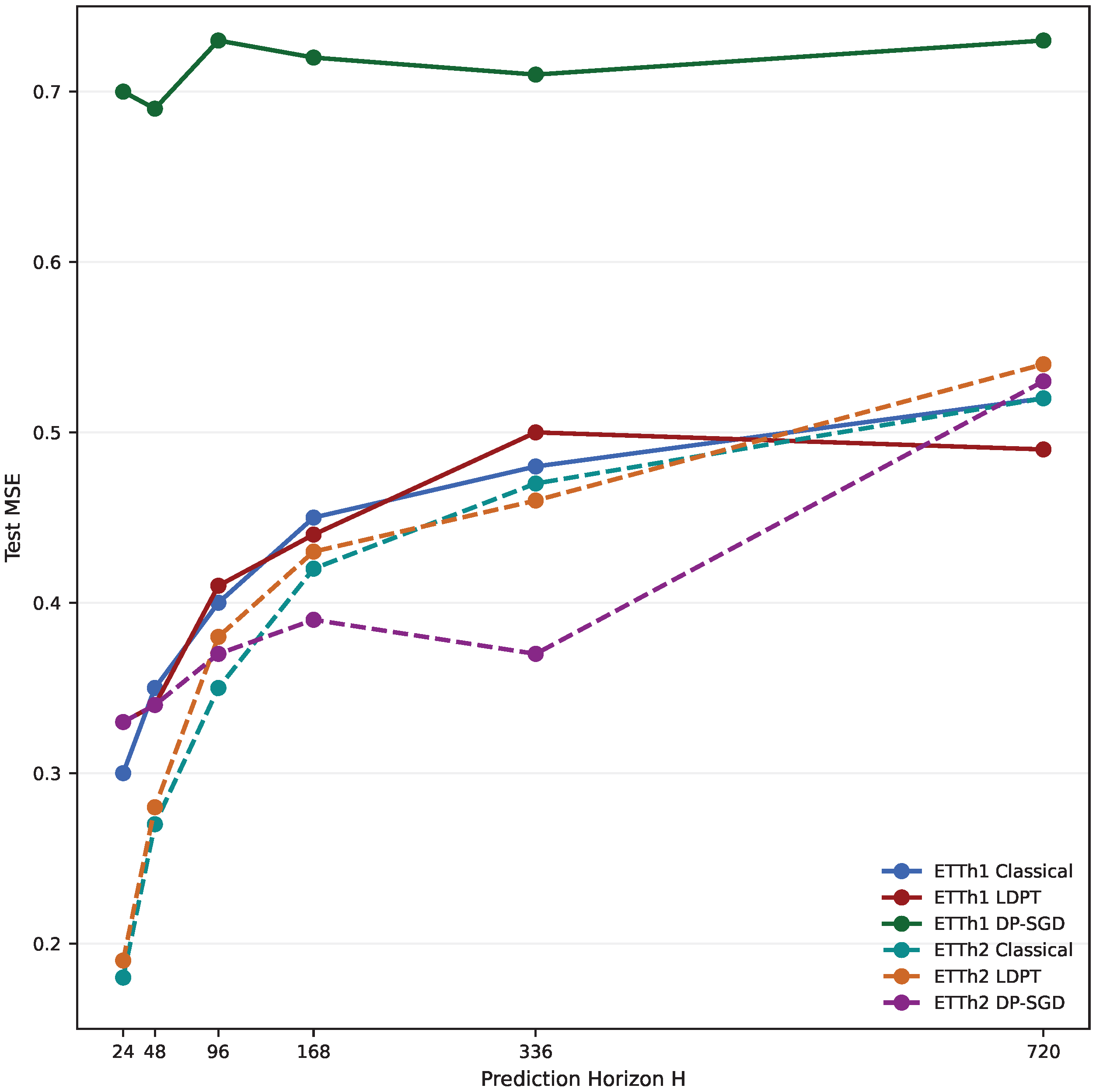
8.1. Feature-Path vs. Gradient-Path Privacy
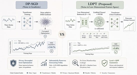
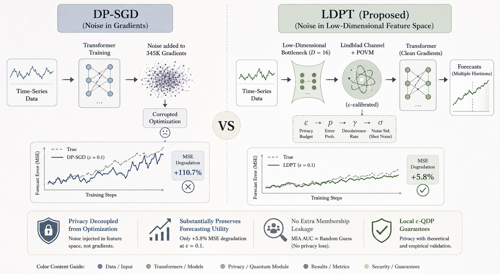
Privacy perturbations are substantially less destructive when separated from the optimization gradients and confined to a low-dimensional feature representation. For larger models, this dimensional separation grows: doubling
P doubles DP-SGD’s noise burden but has zero effect on feature-path noise. Under feature perturbation
, the induced gradient perturbation is
The expected gradient error is then bounded by
which depends on
D, not
P. In contrast, DP-SGD’s gradient perturbation satisfies
(Proposition 1). This explains the training convergence data in
Table 4: LDPT’s training loss (
) matches Classical because the optimizer receives near-clean gradients, while DP-SGD’s training loss (
) stalls near random initialization because each update is dominated by noise.
Over
T training steps, the cumulative noise variance is
for DP-SGD versus
for LDPT. Since
, the per-step noise is orders of magnitude smaller for feature-path injection even before accounting for the Jacobian attenuation. This is consistent with the 3–
lower seed-to-seed variance observed in
Table 11: gradient noise compounds stochastically across the full 345 K-dimensional optimization trajectory, while feature noise perturbs only the 16-dimensional representation.
The generalization implications follow directly. Under standard noise-stability arguments [
2], the generalization gap scales with the noise injection dimension:
For
,
K, and
, the feature-path bound is
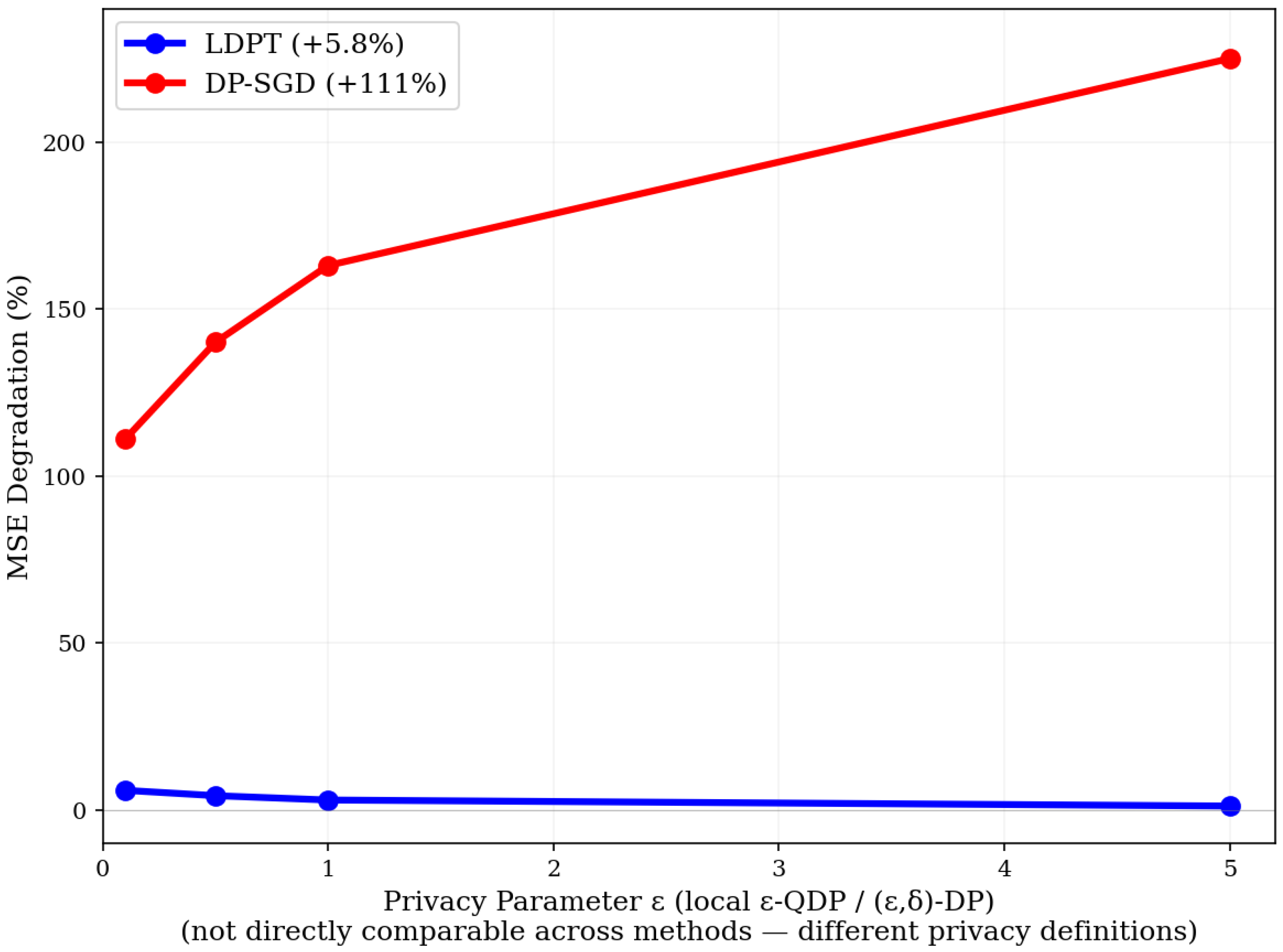
tighter. This is consistent with the empirical observation that LDPT maintains near-baseline test MSE (
), while DP-SGD’s test MSE doubles (
), and explains why the MIA evaluation (
Section 7.11) shows near-zero generalization gap for LDPT (
) versus large gaps for DP-SGD (
) and Bottleneck-DP (
to
).
8.4. Classical Bottleneck Ablation: Separating Architecture from Calibration
Two ablation experiments disentangle the architectural and calibration contributions.
Table 14 isolates noise placement by matching LDPT’s
without any privacy guarantee.
Table 15 tests whether classical
-DP calibration can replace the QDP calibration at the same privacy level. Together, they show that noise placement determines utility, while the calibration mechanism determines the achievable privacy–noise tradeoff.
For
Table 14, we run the identical transformer backbone with
use_quantum=False (no Lindblad channel, no POVM, no quantum features), but with the three-point noise injection active at the
same magnitudes as LDPT.
Table 14 is a diagnostic, not a head-to-head comparison: the bottleneck rows use LDPT’s noise scale
but carry no privacy guarantee (Privacy column = “none”).
Within this controlled setting, the classical bottleneck matches or slightly outperforms LDPT’s MSE at every horizon and
value, isolating noise placement as the architectural factor responsible for utility preservation. The bottleneck even outperforms the no-noise baseline, indicating that low-dimensional noise also acts as a regularizer. The small ETTh1 gap between Bottleneck (e.g.,
at
,
) and LDPT (
) is the utility cost LDPT pays for carrying a formal
-QDP guarantee, while the Bottleneck has none; this gap shrinks to zero on ETTh2 (
Table A5). Crucially,
Table 14 does not imply that the calibration is unnecessary—it only shows that utility is determined by placement, not by the noise source. The calibration question is answered by
Table 15.
However, utility alone is not sufficient for privacy-preserving systems. The classical bottleneck as implemented provides no mechanism-specific mapping between noise magnitude and a privacy parameter ; one cannot compute what privacy level the noise scale provides without a bound analogous to Theorem 1. It therefore cannot support formal privacy guarantees, compositional privacy accounting, or auditable privacy budgets. In contrast, the quantum-inspired framework provides a principled calibration mechanism where directly determines all noise parameters via the QDP bounds (Theorems 1–3), enabling formal -level guarantees and verifiable budget tracking.
These results demonstrate that effective privacy-preserving learning requires both components:
Architectural placement of noise in a low-dimensional feature path to preserve utility, confirmed by the bottleneck achieving near-baseline MSE.
Mechanism-specific calibration to provide formal privacy guarantees—provided by the Lindblad/POVM framework via Theorems 1–3.
Removing either component leads to failure: calibration without architectural decoupling (DP-SGD) yields MSE degradation; architecture without calibration (bottleneck) yields noise of unknown privacy strength. LDPT combines both, achieving MSE with formal QDP.
To verify that the QDP calibration is not merely decorative, we ran a second bottleneck experiment, the same classical architecture, but with noise calibrated via the standard Gaussian mechanism (, sensitivity , ). This gives the bottleneck formal -DP, a direct comparison with LDPT on privacy, not just noise scale.
Table 15 reveals why the calibrated channel formulation is not decorative. The Gaussian mechanism requires
to achieve
-DP, producing catastrophic MSE (
K—the model diverges to degenerate predictions). LDPT achieves
-QDP with
—substantially smaller perturbation magnitudes—because the depolarizing channel bound (Theorem 1) provides a tighter
-to-
mapping than the classical Gaussian mechanism for this architecture. Even at
, the Gaussian-mechanism bottleneck (
, MSE
) substantially underperforms LDPT (
, MSE
). The two calibration mechanisms converge only at weak privacy (
), where both require little noise. This gap is not dataset-specific: on ETTh2, Bottleneck-DP at
produces MSE
K, while LDPT achieves
(
Table A3 and
Table A4,
Appendix A).
The ratio of required noise scales (
vs.
) reflects incompatible sensitivity assumptions and should not be interpreted as a direct quantitative comparison. The Gaussian mechanism uses worst-case
-sensitivity
, while QDP assumes trace-distance bound
in a different metric space. Nevertheless, an approximate decomposition is informative. The Gaussian mechanism in
Table 15 uses worst-case sensitivity
, while QDP assumes trace-distance bound
. These quantities live in different spaces (
on classical features vs.
on density matrices), so a direct rescaling is not rigorous; however, as an indicative comparison, if the Gaussian mechanism were applied with sensitivity reduced to the bounded-perturbation regime (
), its required noise would drop from
to
—accounting for roughly
of the gap. The remaining
(
vs.
) is consistent with a tighter geometric calibration of the depolarizing channel on low-dimensional bounded-purity states under the bounded trace-distance assumptions (Theorem 1): even under this non-rigorous decomposition, the Gaussian mechanism requires approximately
more noise than the depolarizing-channel calibration. A formal decomposition would require deriving the induced
-sensitivity of the amplitude encoding under the trace-distance constraint, which we leave to future work. The Bottleneck-DP row at
exhibits non-monotonic MSE relative to
, consistent with seed-level variance in a regime where
is small relative to natural data variance; this does not affect the central
finding.
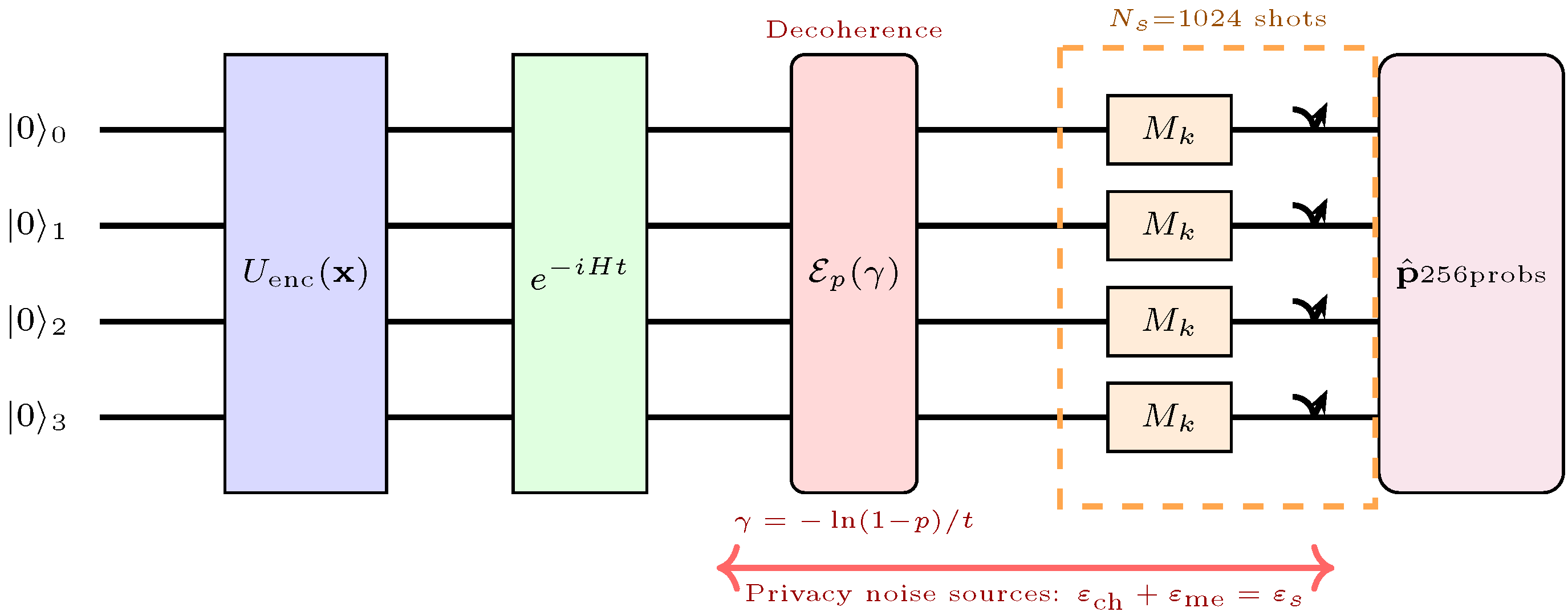
Table 16 compares the per-epoch training cost. LDPT’s overhead comes from the quantum feature pipeline: Lindblad propagation (
matrix-vector multiply per sample), SIC-POVM measurement (
inner products), and shot noise sampling. The Liouvillian
is precomputed once (
for matrix exponential) and reused across all samples and epochs, amortizing to negligible per-sample cost. In practice, the quantum path adds
wall-clock overhead versus the Classical baseline on A100, while DP-SGD adds
(gradient clipping + noise). DP-Input has no overhead beyond a single
randn_like per batch.
8.6. Limitations
While LDPT demonstrates strong empirical results on the ETT datasets, several limitations should be noted.
Experiments were conducted exclusively on ETTh1 and ETTh2 (electricity transformer data,
, hourly frequency). These datasets are relatively low-dimensional and stationary, and the calibration chain assumes z-score normalized features with bounded trace distance. Performance on higher-dimensional or highly non-stationary datasets—e.g., MIMIC-III clinical vitals, intraday financial returns, or weather data with abrupt regime shifts—may differ, particularly because non-stationary distributions can produce per-feature perturbations exceeding the
trace-distance bound (
Section 6.2). Whether LDPT’s calibration degrades gracefully or requires recalibration to a larger
d in such regimes is an empirical question we plan to address in future work, alongside ETTm1, weather, and clinical benchmarks.
The current implementation uses qubits (), resulting in a manageable Liouvillian matrix. Scaling to () produces a matrix, which requires GB of FP64 memory for the Liouvillian matrix exponential alone and dominates the per-experiment cost. Approximate techniques (feature subsampling within the bottleneck, parallel small circuits, or Trotterized propagation) will be required for .
LDPT provides
local -QDP under a bounded trace-distance assumption (
). This bound holds reliably for small perturbations (
standard deviations per feature; see
Table 2) but does not cover arbitrary record additions, removals, or large changes, as in the standard global
-DP adversary model used by DP-SGD. The guarantee degrades gracefully for pairs exceeding the trace-distance bound. Consequently, direct comparisons of privacy strength with global DP mechanisms should be made with caution. We primarily use the DP-SGD baseline to highlight the impact of noise
placement, not to assert strictly superior privacy.
All experiments were performed on a single A100 GPU with a limited compute budget. This restricted us to two datasets, three random seeds, and focused multi-seed validation on two horizons. While results at for MIA are representative (as the attack relies on model-level generalization gaps), broader validation would increase confidence.
Predictions are stochastic at inference time due to ongoing noise injection and finite-shot measurement. Additional comparisons with other feature-level or representation-level privacy methods (e.g., DP-FTRL, locally private representations) would be valuable. A finer-grained residual analysis comparing LDPT, DP-SGD, and Classical predictions across horizons—characterizing residual bias, variance scaling with forecast step, and lag-k autocorrelation—would clarify whether feature-path and gradient-path noise produce structurally different error distributions. We leave this characterization to future work.