Article

Desirability Rating-Based Counterfactual (DeRaC) Framework for Complex Multi-Output Classification Problems


Department of Computer Science and Engineering, University of Louisville, Louisville, KY 40292, USA
*
Author to whom correspondence should be addressed.
Mach. Learn. Knowl. Extr. 2026, 8(4), 109; https://doi.org/10.3390/make8040109
Submission received: 13 February 2026 / Revised: 16 April 2026 / Accepted: 17 April 2026 / Published: 19 April 2026
(This article belongs to the Section Learning)

Abstract

Counterfactual explanations are increasingly vital for understanding and trusting machine learning models. This paper presents Desirability Rating-based Counterfactual (DeRaC), which is a generalized framework for generating valid counterfactual explanations applicable to classification problems with complex output spaces, including single and multi-output classification with binary and multi-class outputs. By expanding the definition of counterfactual validity through a novel “desirability rating,” the approach addresses limitations in existing methods regarding complex output spaces. The framework introduces concepts such as partially valid counterfactuals and a quantitative measure of output desirability. It can be integrated with various objective functions to identify counterfactuals that satisfy properties such as similarity, proximity, and validity. Experiments demonstrate the feasibility of systematically generating counterfactuals using existing optimization techniques, achieving varying degrees of validity and similarity; specifically, Genetic Algorithm produces consistently higher counterfactual desirability albeit at the expense of longer computation times. We observed a higher average counterfactual desirability rating of 0.871 across all tested optimization methods with Powell’s method combined with DeRaC achieving the lowest average distance of 0.897 when using a mixed-objective function. The research emphasizes the context-dependent nature of counterfactuals and lays the foundation for more transparent and trustworthy machine learning systems.

1. Introduction

Machine learning and artificial intelligence models are increasingly being deployed in decision-making and decision-assisting systems across critical domains like finance (credit, insurance, e-commerce, etc.) [1], law enforcement (facial recognition) [2], and cybersecurity (threat detection) [3], among others. These models often utilize complex algorithms, sometimes operating as “black boxes” where their internal workings are opaque. Explaining these AI-ML systems is challenging yet crucial for building trust, identifying biases, and ensuring fairness. A prominent technique within eXplainable Artificial Intelligence (XAI) is post hoc explanation, which focuses on understanding model decisions rather than the models themselves; among these, counterfactual explanations [4] have emerged as a widely used method.
Rather than providing a global view of the model, counterfactuals offer a contrastive explanation by answering the question: “What is the smallest change required in the input to change the model’s output?” By identifying these minimal perturbations, counterfactuals effectively probe the model’s local decision boundary, revealing which features are most influential for a specific decision. This transforms the explanation from a static observation into an actionable roadmap, providing users with a clear understanding of the causal-like relationship between their input attributes and the resulting prediction.
Counterfactual instances are generated from a specific sample instance that has received a particular prediction from a model. They represent instances with minimal differences from the original instance, which are designed to yield a predetermined, or “desired,” output. In Figure 1, a classification model b1 predicts “electrical failure” based on features “predictor1” and “predictor2”. Given that the region inside the model b1 represents positive classifications, instance x receives a positive prediction. If the desired output is negative classification, x″ achieves this while x′ does not, rendering x″ a “valid” counterfactual and x′ an “invalid” one [5]. A typical counterfactual algorithm takes the original instance (x), the prediction model (b1), and the desired output as input, seeking a solution that balances proximity to the original instance with adherence to the desired prediction while considering factors like proximity, actionability and similarity.
While counterfactual explanations offer a powerful means of understanding AI/ML model decisions, their practical application is hampered by challenges in high-complexity output spaces. Many of the existing definitions often rely on very loose definitions of “validity”, requiring a counterfactual instance simply to “change” the original output [4,5]. For instance, implementations such as DiCE [6] focus on actionable recourse; however, they struggle with complex multi-output classification problems. The definition of a “different” outcome is particularly ambiguous in classification with complex output spaces, as multiple distinct outcomes may exist, and these outcomes are frequently not equal in desirability or utility. If the definition of a ‘valid’ outcome is imprecise, the resulting explanation may be misleading or irrelevant to the user’s actual needs, undermining the utility of the counterfactual as an explanatory tool. This ambiguity is discussed in further detail in Section 2. We propose a new framework to expand the definition and methodology of counterfactual generation to handle the nuances of complex multi-output classification. Our contributions, therefore, lie in the following:
1.
Formalizing the DeRaC framework for counterfactual generation in complex multi-output classification problems;
2.
Establishing and demonstrating the utility of partially valid counterfactuals;
3.
Optimizing counterfactual generation based on critical properties for classification problems with complex output spaces;
4.
Comparing DeRaC against existing counterfactual generation methods, specifically within the context of complex multi-output classification.

2. Ambiguity of Counterfactual in Complex Multi-Output Classification Problems

While counterfactual explanations are well established for single-output classification, applying them to high-complexity output spaces, encompassing multi-class, multi-output, and combined structures, introduces significant ambiguity. In traditional binary classification, finding a “different” prediction is sufficient to define a “valid” counterfactual. However, this approach becomes inadequate when dealing with multiple classes or outputs as the explanatory value of a counterfactual depends entirely on whether the alternative state reached is meaningful within the problem’s specific context.

2.1. Multi-Class Classification Problems

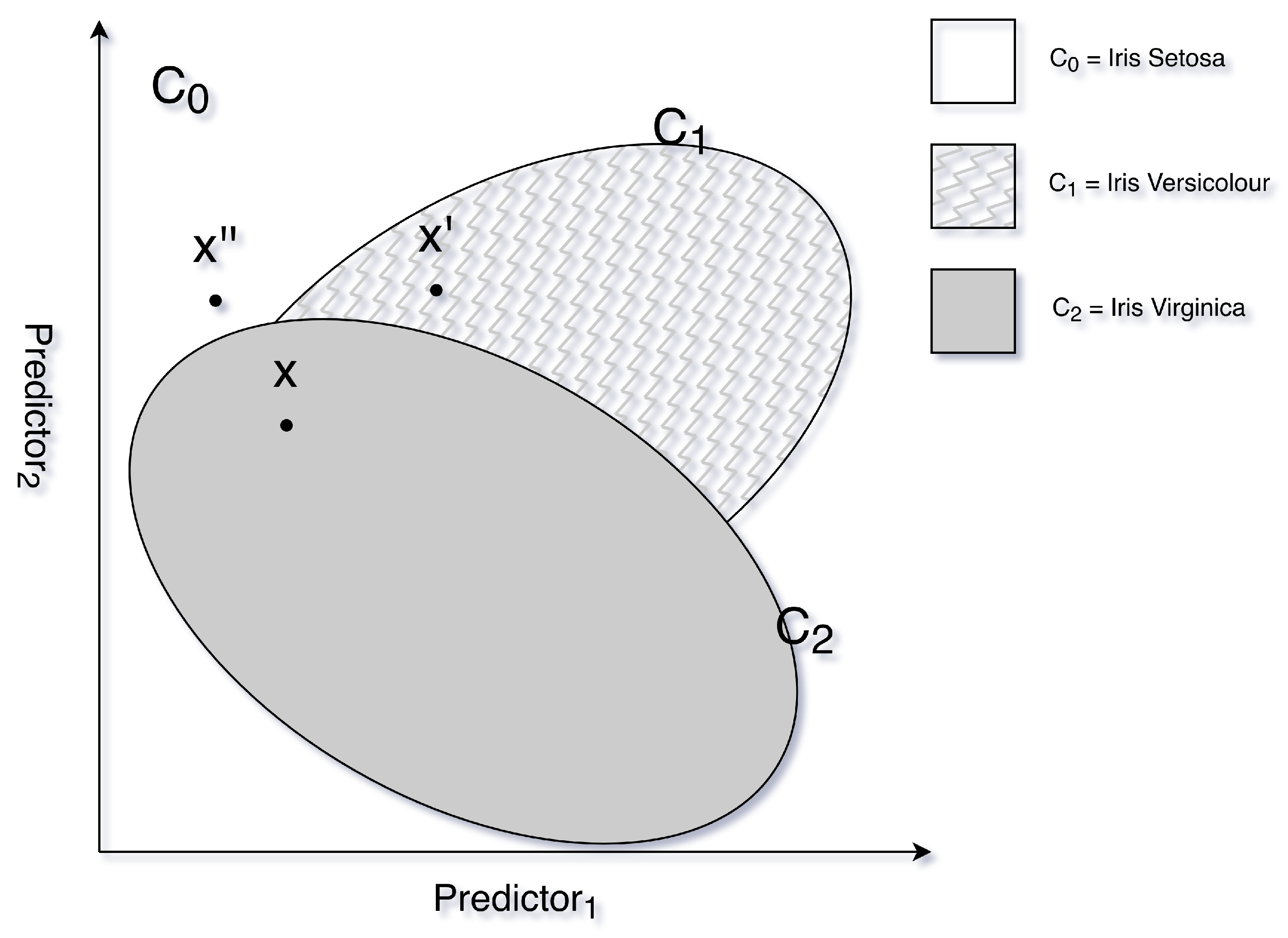
Consider a multi-class classification problem, such as the Iris dataset [7], where the target variable “class” consists of three categories “Iris Setosa”, “Iris Versicolour”, or “Iris Virginica”. As shown in Figure 2, an instance (x) with a predicted class of C2 has two possible “different” predictions. Treating all these as equally “valid” counterfactuals overlooks the nuance of their utility. The validity of a counterfactual hinges on achieving a “desirable” output, which is context-dependent and tied to the original instance and specific use case. Furthermore, multi-class problems involve categorical classes that are mutually exclusive; an instance can belong to only one class at a time.
Multi-class problems can be further categorized into nominal and ordinal classifications. In nominal problems, classes have no inherent order (like the example above with the Iris dataset [7]). However, in ordinal problems, classes have a defined order, impacting the assessment of desirability. For example, in the frequently used Wine Quality dataset [8], a prediction of 7 is more desirable than 4 if the goal is to achieve a higher value (such as 9).

2.2. Complex Multi-Output Classification Problems

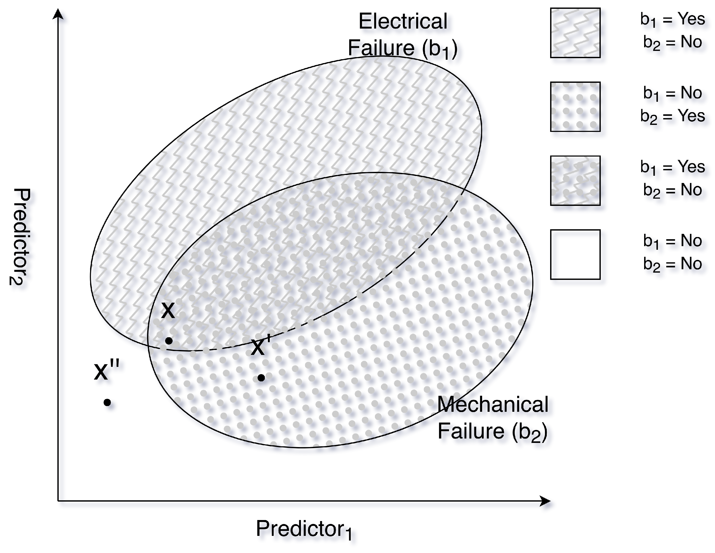
Beyond multi-class scenarios, we encounter multi-output classification, where multiple independent classifiers predict different outputs, as illustrated in Figure 3. Unlike multi-class problems, outputs in multi-output scenarios are not mutually exclusive. A combination of both multi-class and multi-output structures forms complex multi-output classification problems. The core challenge remains consistent: simply finding a “different” prediction is insufficient. The validity of a counterfactual depends on achieving a combination of desirable outcomes across all outputs, which requires defining and quantifying what constitutes a “desirable” state for each dimension and the overall problem. Therefore, a more robust framework for evaluating counterfactual validity is necessary for effective explanation in these complex scenarios.
This gap leaves fundamental concepts, such as “desired vs. undesired” outputs and “valid vs. invalid” counterfactuals ill defined within classification systems with complex output spaces. To address this, this paper formalizes counterfactual explanations for any combination of multi-class and multi-output problems, introducing the notion of partially valid counterfactuals and demonstrating their utility in model interpretability. We further present an optimization framework for generating these counterfactuals, incorporating key properties such as validity, proximity, and similarity.

3. Literature Review

A critical field of research that has emerged in recent years is eXplainable Artificial Intelligence (XAI), which is driven by the increasing deployment of complex AI systems across diverse applications [9]. The core challenge of XAI lies in bridging the ‘black box’ nature of many AI models, particularly deep learning, by providing humans with understandable explanations of how these systems arrive at their decisions. According to Ali et al. [10], this landscape can be divided into data explainability (focused on explaining the training data through training and AI models), model explainability (focused on creating AI models that are naturally more explainable), and post hoc explainability (focused on explaining AI model decisions after the fact). More recently, research has increasingly centered on counterfactual explanations—a post hoc explanation method—which offer a specific approach to addressing this challenge by identifying the minimal changes to an input that would alter a model’s prediction [5].

3.1. Problems with Complex Output Spaces in Machine Learning

Multi-class and multi-output problems are increasingly prevalent in various fields, driving significant research into machine learning solutions. These problems involve predicting multiple outputs simultaneously, moving beyond traditional single-target prediction. As highlighted in several studies, this approach is crucial for tasks like predicting chemical parameters of river water quality from biological data [11], forecasting blood-drug concentrations in time-series data [12], and estimating multiple biophysical parameters from remote sensing images [12]. The ability to model relationships between multiple dependent variables offers more comprehensive and accurate predictions than treating each output in isolation.
Machine learning techniques, particularly regression trees and their ensembles, are frequently employed to tackle these complex problems. Researchers have explored methods like multi-target regression trees, model trees with linear models in leaves, and adaptations of multi-class classification techniques for regression tasks [13]. These methods aim to capture the correlations between different outputs and improve predictive performance. Furthermore, problem transformation methods convert multi-target regression into multiple single-target problems, offering another avenue for solution [13]. The use of algorithms like support vector regression, ridge regression, and even simpler approaches like linear regression demonstrate the versatility of machine learning in this domain [13,14].
The effectiveness of these machine learning approaches in regression domain is validated through rigorous evaluation metrics such as correlation coefficients and root mean squared error (RMSE), which are often assessed using cross-validation techniques [13]. The small confidence intervals observed in some studies indicate the stability and reliability of these algorithms when applied to sufficiently large datasets. This demonstrates the growing importance of machine learning in addressing multi-output and multi-class challenges, enabling more informed decision making and deeper insights in diverse application areas.

3.2. XAI and Introduction of Counterfactual Explanation

Wachter et al. [15] introduced counterfactual explanations as a novel paradigm within the XAI field. The paper argues that the explanations of model decisions should focus on external factors that can be changed rather than focusing on internal workings of the algorithms. A counterfactual of an instance x classified by a model b as y = b(x) is an instance x′, where the model’s decision is different; i.e., b(x′) != y, and the difference between x and x′ is minimal [4,5]. A counterfactual explainer [5] is a function that takes a classifier b, known instances X, and an instance x and returns a set of ‘valid’ counterfactual examples C = { x 1 , …, x h } such that b( x i ) != b(x) for all x i in C.
These definitions are primarily centered around changing a single prediction outcome (b(x′) != b(x)) for a specific instance, as is typical in classification, where the output is a single class label. The Guidotti survey [5] explicitly states that its analysis and categorization focus on counterfactual explanation methods designed to explain black-box classification models because the large majority of the literature addresses this problem. Despite a number of surveys [4,16,17,18,19,20] that have explored benchmarking, identified deficits, and conducted analyses of existing counterfactual explanation research, a common thread emerges: almost all of these studies predominantly assess single-output binary classification problems. Guidotti [5] also defines the properties of desirable counterfactuals which are summarized in Table 1.

3.3. Current Techniques for Counterfactual Generation

While the foundational concepts of counterfactual explanations have been established [15], a diverse range of methods have been developed to generate these explanations in practice. Many approaches formulate the search for counterfactuals as an optimization problem, aiming to find the smallest perturbation to an input that flips the model’s prediction. Various approaches such as [21,22,23] focus on different methods of using generative adversarial networks to generate counterfactuals. Several studies have investigated different ways to efficiently solve the objective function and calculate counterfactuals such as using fuzzy decision trees [24], solving for multiple constraints [25], using ensemble methods [26], using program synthesis [27], or solving other problems of optimizing [28,29,30].
Various approaches have focused on developing tools to generate counterfactuals such as the decision explorer (DECE) by Cheng et al. [31], which is an interactive framework to allow users to explore model decisions and generate counterfactuals. There are also tools like DiCE developed by Mothilal et al. [6] that generate a diverse set of counterfactuals and are widely used for both classification [32] and regression [33]. The what-if tool (WIT) [34] and language interpretability tool (LIT) [35], both developed by research teams at Google Research, offer functionalities directly related to counterfactual explanations. WIT allows users to automatically identify counterfactual examples, aiding in understanding model decisions. Similarly, LIT provides first-class support for counterfactual generation, enabling users to add new data points and immediately visualize their effect on model predictions, and it also facilitates side-by-side comparisons. These tools acknowledge the importance of counterfactuals as a method for interpreting model behavior and offer practical ways to explore these explanations.
There are other tools that help to visualize and explain classifiers using counterfactuals such as Prospector [36], RuleMatrix [37], SystemD [38], ViCE [39], and WiXAI [40]. Significant research has also addressed non-tabular data, such as images, text, and time-series datasets. Works such as [41] focus on visual counterfactuals identifying how an image could be changed to alter a vision system’s prediction. Their method involves finding regions in a ‘query’ image and a ‘distractor’ image (predicted as the desired alternative class) and swapping them to shift the prediction. This is distinct from simply highlighting important features; it focuses on minimal edits to achieve a different outcome. Other research works include [42,43,44,45,46,47]. For text, research focuses on automated counterfactual generation, acknowledging the challenge of maintaining natural language while making minimal changes such as [48]. These tools and techniques collectively highlight the growing interest in leveraging counterfactual explanations for model debugging, fairness analysis, and increased transparency in machine learning systems.

3.4. Applications and Extensions of Counterfactual Explanations

Beyond the core definition and generation of counterfactuals, research in this area is diversifying into several key directions. Research has also focused on enhancing the quality of counterfactuals, emphasizing plausibility, actionability, and diversity. For instance, Arie et al. [49] propose optimizing counterfactual-based analysis through the use of databases, while Piccialli et al. [50] propose utilizing counterfactual explanations to detect important decision boundaries and training a more compact easily explainable model like decision tree that closely resembles the original black-box model. Artelt et al. [51] present a case study where counterfactuals are generated for groups rather than each individual to provide actionable recommendations for businesses while reducing the complexity of counterfactual generation. Gao et al. [52] present a self-training model that uses pseudolabels generated from a base classification model that uses those pseudolabels to retrain combined with factual data. Their method is iterative and uses counterfactual virtual adversarial training (CVAT) to ensure the models do not get stuck with incorrect guesses.
Furthermore, Temraz et al. [53] present an interesting approach to solving issues with imbalanced datasets by using counterfactual augmentation (CFA). The CFA method generates counterfactuals based on the factual dataset in the minority class, thus producing synthetic data points rather than oversampling. Another interesting approach by Sohns et al. [54] involves a method of visualizing a decision boundary for counterfactual reasoning using local linear maps of the decision space and combining it with other model inspection techniques. Our previous work [40] also created a tool, WiXAI, that allows users to explore the decision boundaries via an interactive and iterative visual perturbation of samples, which can help move them toward causal understanding of the relationship between features at a sample level.

3.5. Counterfactual Explanation for Causal Understanding

Since Wachter et al. [15] introduced counterfactual explanations, they have been increasingly recognized for their potential to enhance interpretability within the context of causal inference. These explanations, which detail how an input would need to change to achieve a different outcome, are not merely about prediction but also offer insights into the underlying causal mechanisms [55]. Researchers emphasize the importance of ensuring these counterfactuals are feasible, reflecting real-world constraints and causal relationships rather than simply statistical likelihood [55,56,57]. Generating feasible counterfactuals necessitates moving beyond statistical approaches and explicitly incorporating causal models [55], acknowledging that changes to input features must adhere to natural laws and feature interactions [56].
Recent work focuses on formulating feasibility as a causal concept, demanding that counterfactual perturbations respect the causal structure between input features [55]. Approaches like CEILS aim to bridge the gap between XAI counterfactuals and causal counterfactuals, generating explanations that are both interpretable and actionable by providing causally feasible actions [58]. Evaluating these explanations requires metrics like causal-constraint validity, which assesses the proportion of counterfactuals aligning with domain knowledge and causal frameworks [56], highlighting the shift toward more robust and reliable counterfactual generation for causal understanding.

3.6. Counterfactual for Complex Multi-Output Classification Problems

Despite the evident use of machine learning techniques in solving multi-class and multi-output problems, the application of counterfactual explanations remains relatively sparse in this domain. Most of the existing literature focuses primarily on single-output binary classification. Consequently, the standard definition of ‘changing the output’ is often considered sufficient for identifying counterfactuals in these contexts. Existing research papers that work with non-binary classification problems, such as the work by Carlevaro et al. [59] on multi-class classification problems, follow the same idea of “different output” to define valid counterfactuals. Any classification that is different than the original prediction is treated as a valid counterfactual. We will discuss in Section 2 why such a definition can be ambiguous. While methods like those presented in Caron et al. [60] extend to multi-task learning via deep kernels, the focus remains on estimating causal effects and learning policies and not necessarily on generating easily interpretable counterfactuals for each individual output.
Furthermore, the challenge is compounded when considering combinations of treatments, as highlighted by Parbhoo et al. [61]. Addressing the exponential growth of possible treatment combinations necessitates scalable modeling approaches, but it does not inherently solve the problem of generating understandable counterfactuals for each outcome within a multi-output setting. Current work often simplifies the problem by focusing on single-class or single-output scenarios, leaving a gap in understanding how to effectively generate actionable counterfactual explanations when multiple outputs or multiple labels are simultaneously considered.

4. Desirability Rating-Based Counterfactual Framework for Complex Multi-Output Classification Problems—Methodology

Counterfactual explanations offer a powerful approach to understanding model decisions by identifying minimal changes to an input that would lead to a different prediction. These changes are generated relative to an original instance, the decision model, and a specified desired output. Formally, a counterfactual x′ is a minimally perturbed instance of x such that b(x) ≠ b(x′), where b represents the model [5]. A “valid” counterfactual, in this context, is one that is sufficiently close to the original instance while successfully altering the model’s prediction. However, as discussed in Section 2, a more robust framework is needed for complex multi-output classification problems rather than seeking simply a “different” classification. This section details a framework for generating counterfactual explanations specifically designed for classification problems with complex output spaces, outlining how we define and evaluate the “desirability” of counterfactual instances and how we categorize them as “valid” or “partially valid.” It is important to note that this extended framework applies not only to multi-class and multi-output problems but also to existing binary and single-output classification problems.

4.1. Key Definitions and Scopes

Before detailing our DeRaC framework, we establish the fundamental concepts underpinning our approach. These definitions provide a consistent understanding of the problem space and how we approach generating and evaluating counterfactuals.
1. Type of Problem: This refers to the nature of the classification task. We consider a broad spectrum, including the following:
  • Binary Classification: a single output variable with two possible values.
  • Nominal Multi-Class Classification: multiple output classes without inherent order.
  • Ordinal Multi-Class Classification: multiple output classes with a defined order or ranking.
  • Multi-Class Classification: multiple output classes with or without inherent order (includes both nominal and ordinal multi-class classification).
  • Multi-Output Classification: multiple independent output variables, each with its own classification task.
2. Instances: These are the individual data points fed into the model. Formally, an instance x is a vector of features representing a single observation. The quality and relevance of these instances are crucial for generating meaningful counterfactuals. An instance can also be referred to as a sample or data point.
3. Desired Output: This is the target output we aim to achieve through the counterfactual explanation. It can be a single class label (in binary or multi-class classification), a set of labels (in multi-class classification), or a vector of values (in multi-output classification). The definition of the desired output directly influences the search space for counterfactuals and is context-dependent (varying according to the user and the specific use case).
4. Desirability Rating: This is a metric used to quantify how close an instance’s output is to the desired output. The calculation of this rating depends on the Type of Problem as detailed in Section 4.2. This serves as the foundation for our Desirability Rating-Based Counterfactual (DeRaC) framework.
5. Counterfactual Goal: The objective of finding a counterfactual is not merely to change the prediction but to do so with minimal changes to the original instance. Our goal is to identify the smallest perturbation to x that results in an output closer to the desired output, as measured by the desirability rating while adhering to the properties of effective counterfactual explanations as defined in [5].

4.2. Desirability Rating of Outputs and Instances

The goal of the “desirability rating” metric is to measure how desirable the output of an instance is given a predefined “desired” output. For single-output binary classification problems, the rating is binary (representing either ‘desired’ or ‘undesired’). Similarly, for nominal multi-class classification scenarios, since there is no inherent preference between the undesired outputs, the score is also binary, representing a ‘desired’ or ‘undesired’ output. We can see this function of desirability for binary or nominal multi-class classification in Equation (1). Here, a value of 1 represents the class for the ith output, yi, as “desired” and the value 0 represents the class as “undesired”. Si represents the set of classes for the ith output that are considered to be “desired”. For optimization, the binary value based on the output yi can be replaced by the probability function P i ( · ) based on the classification model of the ith output. This is shown in Equation (2), which provides a continuous output suitable for integration into the objective function for optimization. The differentiability of the function d(yi) depends on the classification model, thus affecting the feasibility of common optimization methods such as gradient descent, which depend on the derivative of the objective function.
d ( y i ) = 1 , if y i S i 0 , if y i S i
where S i is the set of desired output classes for the ith output.
d ( y i ) = s S i P i ( s )
where P i ( · ) is the probability function based on the ith classification model b i ( · ) .
In ordinal multi-class classification, the utility of a prediction depends on its proximity to the target class. To capture this, we define a desirability metric, d(·), as shown in Equation (3). This metric calculates the complement of the normalized ordinal distance between the predicted class yi and the set of desired classes Si. Specifically, the term inside the parentheses represents the ratio of the minimum absolute difference in ordinal rank between the predicted class and the nearest desired class to the total range of the ordinal scale. For finding the total ordinal range, we have the term Ci, which represents all possible classes for the ith output. The scaling factor p allows for non-linear adjustments of this distance, where p = 1 yields a linear scale. Unlike nominal or binary classification, where desirability is strictly binary {0,1}, this approach provides a continuous desirability score in the range [0, 1]. In this scale, 1 represents a perfect match, 0 represents the least desirable outcome, and intermediate values represent partial desirability. Optimization can be achieved by minimizing the normalized distance term as formulated in the objective function F(·) in Equation (4).
d ( y i ) = 1 m i n s S i ( | o r d e r ( s ) o r d e r ( y i ) | ) m a x c C i ( o r d e r ( c ) ) m i n c C i ( o r d e r ( c ) ) p
where S i is the set of desired output classes for the ith output and C i is the set of all possible classes for the ith output.
F i ( · ) = m i n m i n s S i ( | o r d e r ( s ) o r d e r ( y i ) | ) m a x c C i ( o r d e r ( c ) ) m i n c C i ( o r d e r ( c ) ) p
As we noted above, the complexity of measuring the desirability of an output depends on the type of output; it results in either a binary value or a ratio between 0 and 1. Similarly, for multi-output problems, we can combine the desirability of each individual output to obtain an overall desirability score for an instance. The most straightforward combination would be to assign equal weights to all the outputs and calculate the proportion of outputs that yield a desired output. It is also possible to assign varying weights to individual outputs depending on the problem. As such, the overall desirability rating of an instance can be measured as shown in Equation (5). In Equation (5), x represents the instance, while yi represents the ith output in an n-output classification space for the given x. Likewise, d(yi) represents the desirability score for the ith output, wi represents the weight assigned to the ith output, and D represents the overall desirability rating of an instance. Consistent with Equation (3), the value can be in the range of [0, 1] with 0 representing an undesired outcome, 1 representing a desired outcome, and intermediate values representing a partially desired outcome.
D ( x ) = i = 1 n ( w i × d ( y i ) ) i = 1 n w i
where y i = b i ( x ) represents the ith out of n outputs based on the classification model b i ( · ) , d ( y i ) represents the desirability of the ith output, and w i represents the weight assigned to the ith output.

4.3. Valid and Partially Valid Counterfactual

As mentioned previously, Wachter et al. [15] describe counterfactuals in terms of desired outcomes, showing which external facts could be altered to attain a desired outcome. A counterfactual is thus framed in terms of “desired” and “undesired” outputs. Counterfactuals are declared ‘valid’ if they reach the desired outcome; otherwise, they are treated as ‘invalid’. For our problem of multi-class and multi-output classification, we encounter not only desired and undesired outcomes but also a spectrum of partially desired outcomes. While in single-output binary classification problems, a counterfactual is considered “valid” if it reaches the desired outcome, in these complex scenarios, it is possible to reach a partially desired outcome. Consequently, we introduce the concept of a partially valid counterfactual. A partially valid counterfactual can be described as a counterfactual that has a desirability rating greater than the original instance but is not completely desired.
D ( x ) > D ( x ) and D ( x ) < 1
Mathematically, this is shown in Equation (6), where x′ represents the partially valid counterfactual, x represents the original instance, and D(·) represents the function to calculate the desirability rating of an instance from Equation (5). A counterfactual that has the same or a lower desirability rating than the original instance can be considered an invalid counterfactual, as it does not “progress” in terms of desirability. Alternatively, if an instance is already ‘desirable’, one can consider a different set of outputs as desired and recalculate desirability to find a valid or partially valid counterfactual for that particular use case.

4.4. Desirability Rating in the Counterfactual Search

The DeRaC framework outlined in Section 4 fundamentally alters the concept of counterfactual “validity” as traditionally defined by Guidotti et al. and others [5]. While existing definitions focus on a binary classification of counterfactuals as simply “valid” (prediction changes) or “invalid”, our approach introduces a spectrum of validity through the “desirability rating” and the categorization of “partially valid” counterfactuals. This moves beyond a simple yes/no assessment and allows for the comparison of counterfactuals (where some are demonstrably “more valid” than others, reflecting the degree to which they approach the desired output).
This added complexity is not merely academic; it unlocks new possibilities for counterfactual explanation generation. Instead of solely seeking any counterfactual that achieves the desired outcome, we can now formulate objective functions that explicitly optimize for higher desirability ratings. This allows us to prioritize counterfactuals that not only change the prediction but do so in a way that is “closer” to the desired output, offering more nuanced and potentially more actionable insights. These insights are especially more important when dealing with complex multi-output classification problems.
Specifically, the desirability rating can be incorporated directly into the objective function used by counterfactual search algorithms. For instance, in an optimization process, the objective could be to minimize a combination of the following:
  • Perturbation Distance: a measure of how much the counterfactual x′ differs from the original instance x (e.g., L2 distance, Manhattan distance). This ensures minimal changes, which is a key principle of effective counterfactuals.
  • Negative Desirability Rating: the negative of the desirability rating for the counterfactual. Maximizing the desirability rating is equivalent to minimizing its negative. This drives the search toward counterfactuals with higher validity.
  • Portion of Features Changed: the fraction of features in x that are different in x′. This encourages minimality: counterfactuals with fewer changes are generally more actionable and easier to understand.
The relative weighting of these terms within the objective function allows for control over the trade-off between minimal perturbation and high desirability. A higher weight on the negative desirability rating prioritizes finding counterfactuals that are as close as possible to the desired output even if it requires slightly larger perturbations.
Furthermore, incorporating the concept of “Partially Valid” counterfactuals opens the door to generating a variety of explanations. By systematically adjusting the acceptance threshold for the desirability rating, we can generate a diverse set of counterfactuals, ranging from those that fully achieve the desired outcome (Valid) to those that represent incremental steps toward it (Partially Valid). This variety is crucial for understanding the model’s behavior in complex scenarios and for providing users with a more comprehensive picture of potential changes.
It is crucial to note that other properties of effective counterfactuals, such as plausibility, similarity, proximity and actionability [5], remain essential considerations. Our DeRaC framework complements these properties by adding a more nuanced, quantifiable dimension of validity, enabling more sophisticated and targeted counterfactual generation strategies.

5. Finding Counterfactual with the DeRaC Framework—Experiments

This section details the experiments conducted to evaluate the feasibility and effectiveness of defining and generating valid counterfactual explanations for complex multi-output classification problems using the proposed DeRaC framework for desirability rating discussed in Section 4. We evaluated our approach on three diverse datasets, focusing on the characteristics of generated counterfactuals with respect to proximity (L2 distance), validity (desirability rating), and optimization success. We compared the performance across different strategies for choosing the desired output for counterfactual generation, thereby simulating various context-dependent desired output scenarios. To demonstrate versatility, the results for high-complexity multi-output classification problems are also contrasted with those from single-output binary classification tasks.

5.1. Datasets Used

To ensure a robust evaluation, experiments were conducted using the datasets outlined in Table 2. These datasets vary in size, dimensionality, and class distribution, providing a comprehensive testbed for the proposed approach.

5.2. Model Training and Complex Multi-Output Classification

To establish a robust standard model for counterfactual generation, we trained four distinct architectures: a Multi-Layer Perceptron (MLP), a Random Forest (RF), a Support Vector Machine (SVM), and a Gradient Boosting Machine (GBM). Each model was trained independently for each output dimension.
To ensure rigorous evaluation and prevent data leakage, we implemented a strict data partitioning protocol. The dataset was first partitioned into a training set (70%) and an independent, held-out test set (30%). The test set was reserved exclusively for the final evaluation of the selected models and was not utilized during the hyperparameter tuning phase. Within the training set, we employed a five-fold cross-validation scheme integrated with a grid search to optimize model performance. In this procedure, the training data were subdivided into five folds; in each iteration, four folds were used for model training, while the fifth fold served as a validation set to evaluate the hyperparameter combinations.
The hyperparameter search space for each architecture was defined as follows:
  • MLP: hidden layer architectures {(32,), (64,), (128,), (64,64,), (128,128,)}, activation functions {ReLU, Tanh}, maximum iterations {200, 499, 999}, and initial learning rates {0.01, 0.001}.
  • Random Forest: number of estimators {100, 200, 500}, maximum depth {5, 10, None}, and minimum samples for a split {2, 5}.
  • SVM: regularization parameter {0.1, 1, 10}, kernel types {RBF, Linear}, and gamma values {0.01, 0.001}.
  • GBM: learning rates {0.01, 0.1}, number of estimators {100, 500}, and maximum depth {3, 5, 10}.
For each output dimension, we selected the model configuration that maximized performance based on the specific task: Root Mean Square Error (RMSE) for ordinal multi-class outputs and a weighted F1-score for nominal classification outputs. All experiments were conducted with a fixed random seed (123) to ensure reproducibility. Following model selection, we created a unified multi-output prediction model by integrating the best-performing models for each output dimension. This ensemble approach allows us to predict all outputs simultaneously, providing a consistent and optimized basis for counterfactual generation. Furthermore, while these architectures provide a robust predictive foundation, the specific choice of model is secondary to the core methodology, as our counterfactual generation framework DeRaC is designed to be model agnostic and can be applied to any underlying classification architecture.

5.3. Different Counterfactual Generation Methods

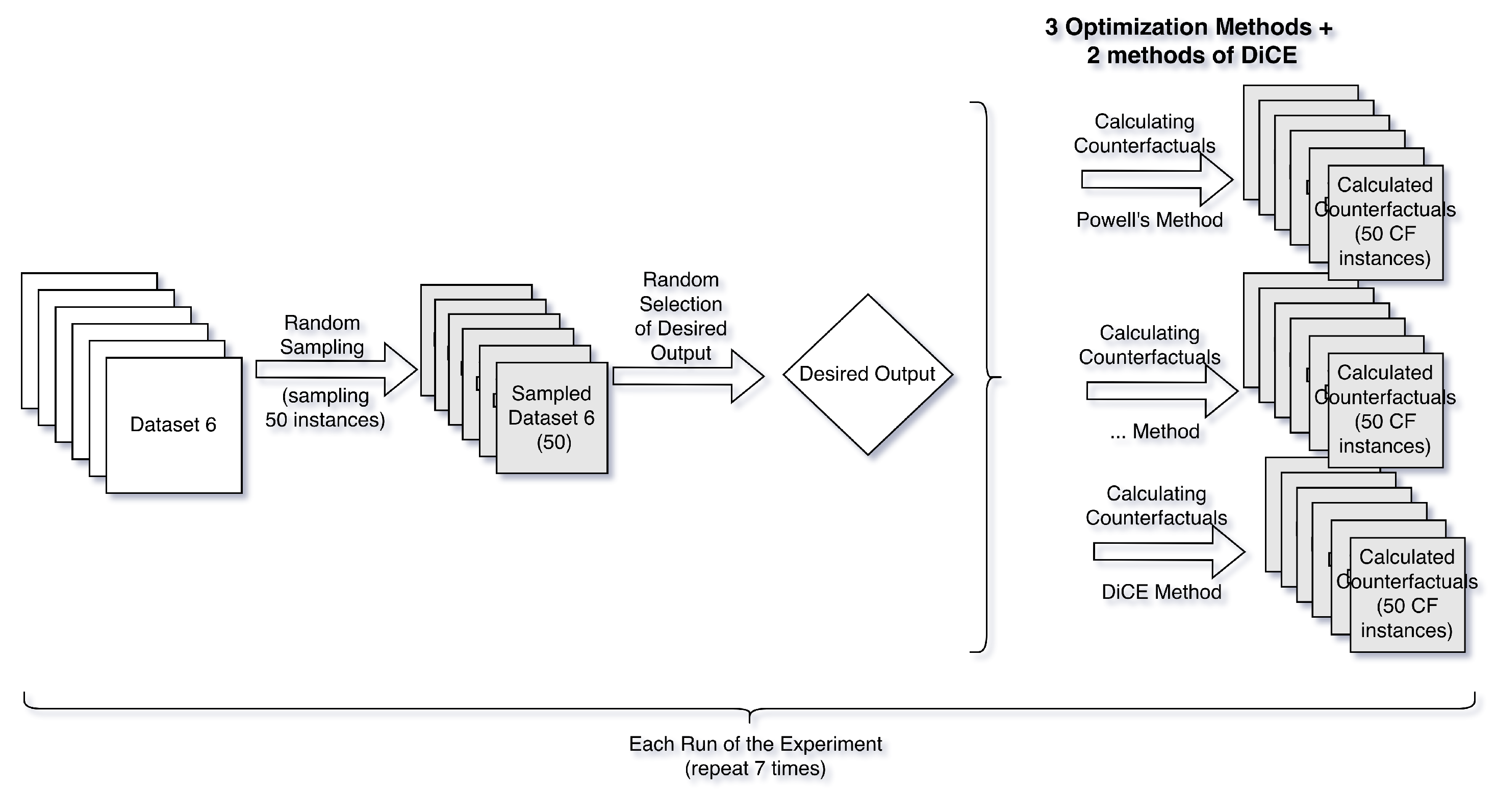
For each sample in the test set, we randomly generated a vector as desired output and applied the following optimization methods to find the corresponding counterfactual. Using the trained model and the selected desired output, we generated a counterfactual instance via the following methods. We used the desirability rating defined in Section 4 to measure the validity (either complete or partial) of the counterfactual instance. We verified the validity of each generated counterfactual by feeding it into the trained model and confirming that the model’s predicted output matched the claimed desirability rating. This process was repeated for 50 randomly selected samples over seven runs for each of the six datasets (as detailed in Table 2), allowing us to assess the robustness of our approach. The experimental schema is illustrated in Figure 4.
1.
Powell’s Method: We employed Powell’s method [65] (implemented via the scipy.optimize library) to find a counterfactual output vector by iteratively searching for a direction of steepest descent.
2.
Nelder–Mead Method: The counterfactual vector was obtained using the Nelder–Mead simplex algorithm [66] (implemented via the scipy.optimize library), which is a derivative-free optimization technique.
3.
Genetic Algorithm (Custom Implementation): We implemented a Genetic Algorithm from scratch to evolve a population of candidate input vectors toward a desired target output.
4.
Genetic Algorithm (DiCE Library): A Genetic Algorithm, leveraging the functionality provided by the DiCE library, was utilized to generate a desired solution through population-based optimization. For generating counterfactuals for multi-output problems, multiple separate counterfactuals are generated for each output, and the counterfactual with the highest desirability rating is selected.
5.
Random Selection (DiCE Library): A random solution was chosen using the random selection functionality within the DiCE library, effectively exploring the feature space without a directed search. Similar to the previous method, multiple separate counterfactuals are generated for each output, and the best counterfactual is selected for multi-output problems.

5.4. Evaluation Metrics

We used the following metrics to evaluate the performance of our counterfactual explanation approach:
Average Distance: 
the average distance between the original input and the generated counterfactual across all samples and experimental runs. Lower distances indicate higher similarity to the original input.
Validity: 
the score assigned by the desirability rating function to the generated counterfactual instances. Higher scores indicate that the counterfactuals more closely align with the desired outcome.
Optimization Success: 
the proportion of counterfactual search processes that resulted in a valid counterfactual. This measures the efficacy of the optimization algorithm in finding successful solutions.
Average Time to Solution: 
the average time (in milliseconds) required to generate a single valid counterfactual. Lower times indicate a more efficient generation process, capturing the computational cost associated with each optimization method.

5.5. Expected Results

We hypothesize that (1) it is possible to systematically define valid and partially valid counterfactuals for complex multi-output classification problems; (2) different optimization strategies will impact the results in terms of time, distance, and partial validity; and (3) existing counterfactual generation methods will struggle when applied to multi-output classification problems. We will combine these results with those obtained for single-output problems to demonstrate the feasibility of our approach in complex multi-output classification scenarios.

6. Results

While we utilized four datasets, two versions were available for both the Student Performance dataset [63] and Wine Quality dataset [8]. Consequently, our experiments included six datasets instead of four. Among the methods tested, Random Forest and Multi-layer Perceptron outperformed the others in these experiments. The scipy library [67] was used to perform the optimization using Powell’s method [65], the Nelder–Mead Method [66], Genetic Algorithm (custom implementation), Genetic Algorithm (DiCE library) [6] and Random Selection (DiCE library) [6]. On each random sample (instance), metrics such as distance, counterfactual validity, desirability rating and computation time were measured.
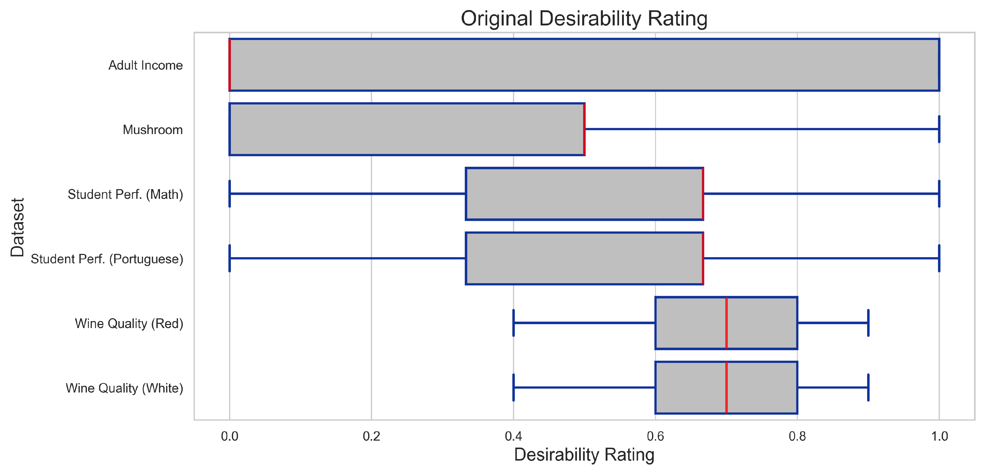
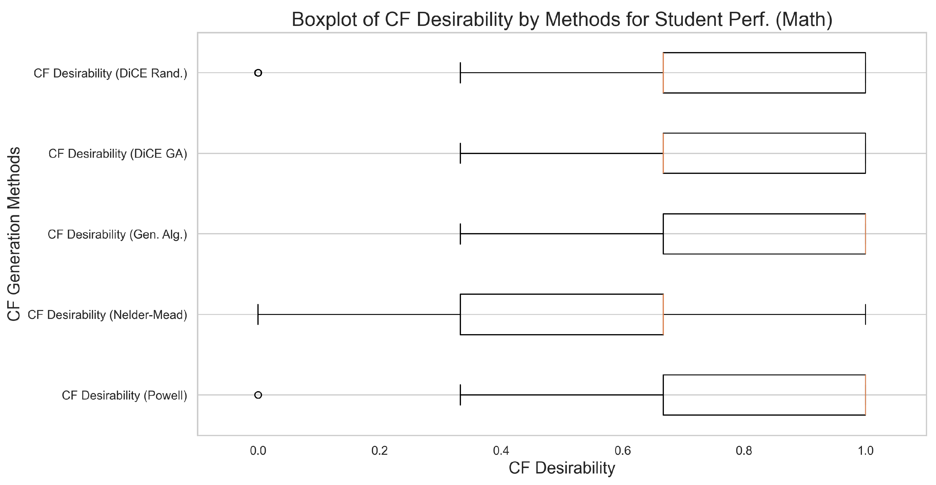
Figure 5 shows the boxplot for the desirability rating of the original samples (instances) randomly selected in our counterfactual generation experiments. The boxplot shows the desirability rating for all the datasets, while the red line marks the mean desirability rating for those samples. Figure 6 displays the boxplot for the desirability rating of counterfactual samples generated via the five different counterfactual generation methods for the Student Performance (Math) dataset. Here, the performance of all methods is comparable except for the Nelder–Mead method, which performs noticeably worse. This trend persists across other results. Among the other methods, our custom Genetic Algorithm achieves the highest mean counterfactual desirability rating of 1.0.
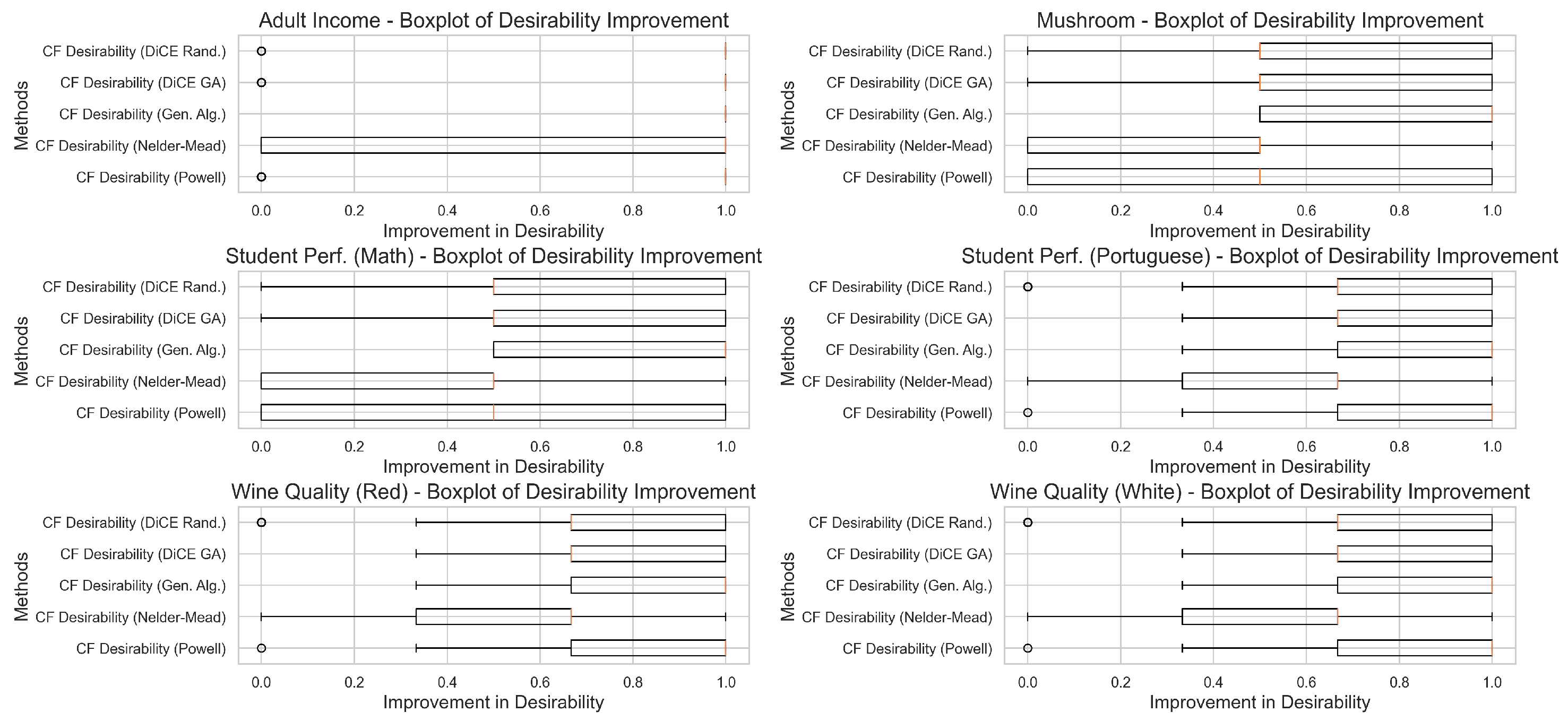
In Figure 7, the boxplots represent the difference between counterfactual desirability and original desirability (where any positive value represents at least partially valid counterfactual). Figure 7 shows that for the single-output binary classification problem (Adult Income [64]), most cases produced valid counterfactuals (our custom Genetic Algorithm failing in no instances). Among all other datasets, the genetic algorithm consistently produced the best average validity in the counterfactual results. This demonstrates that our DeRaC framework systematically generates valid or partially valid counterfactuals and integrates effectively with existing optimization methods. Our framework is also capable of generating valid counterfactuals for both binary classification and complex multi-output classification problems.
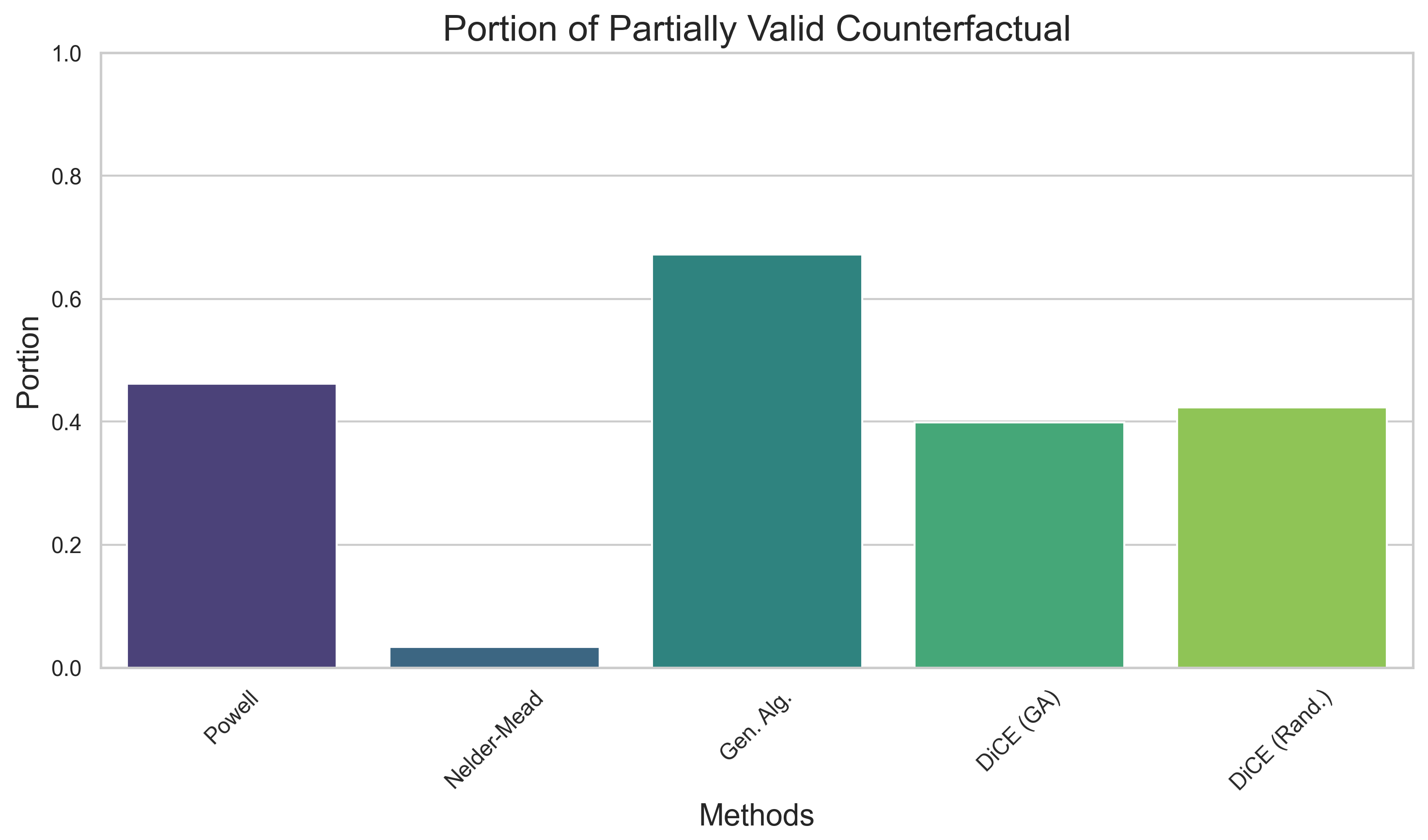
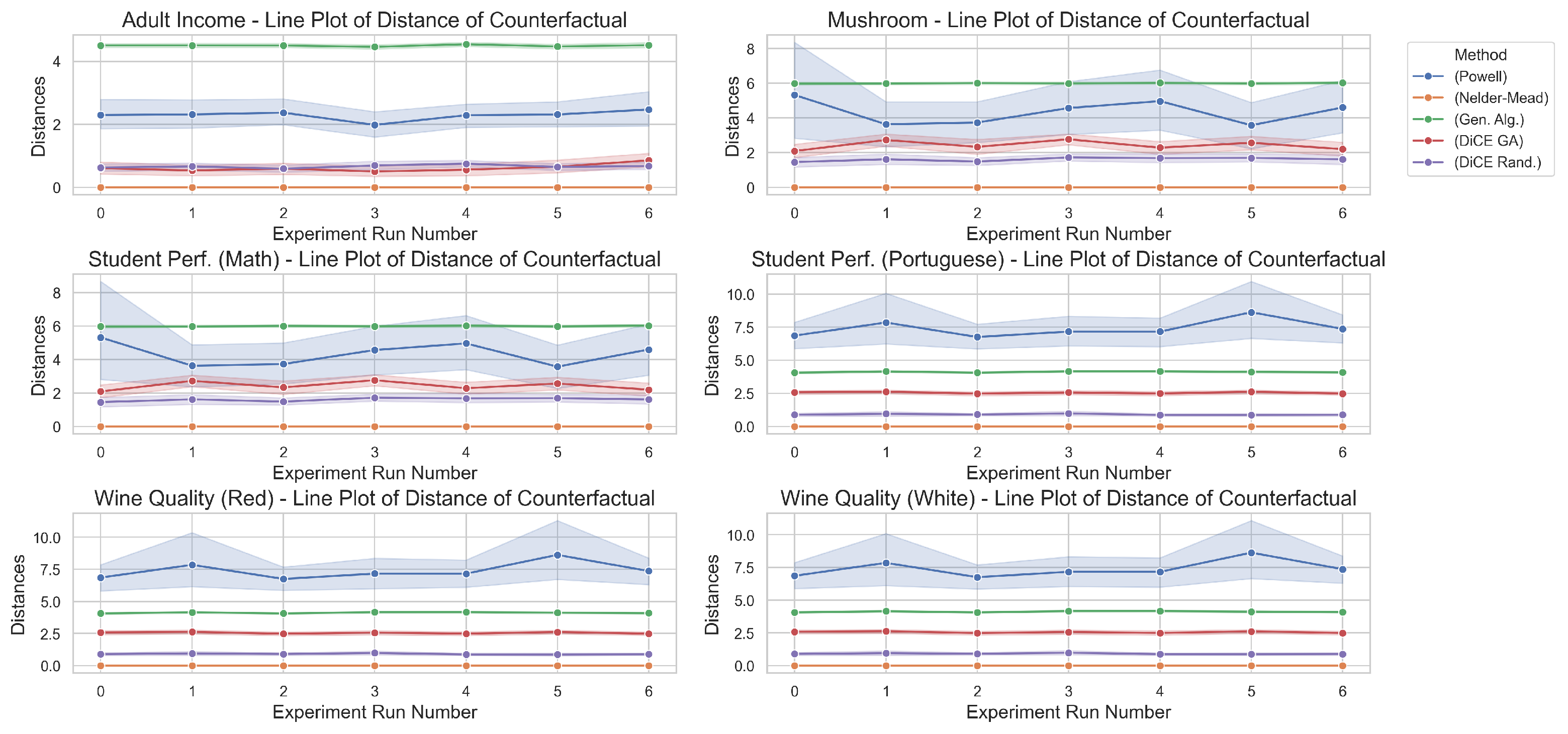
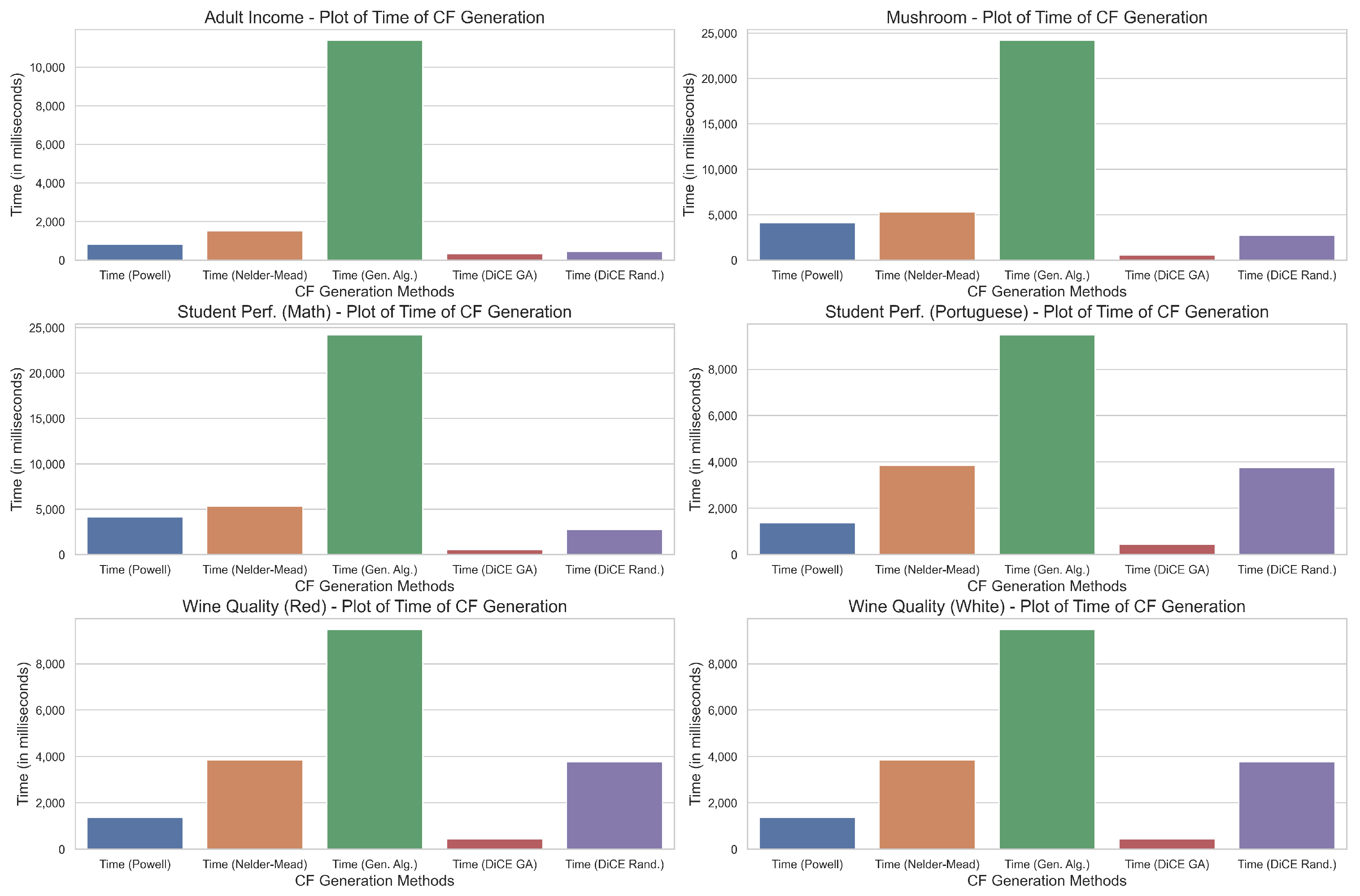
Figure 8 also shows the proportion of valid or partially valid counterfactuals across all datasets and all different runs for each method of optimization/counterfactual generation. The custom Genetic Algorithm performs best with almost 70% of cases resulting in at least partially valid counterfactuals. Powell’s method, DiCE’s Genetic Algorithm and DiCE’s Random Selection closely followed, while the Nelder–Mead method was the least successful. To contrast the success rate, we evaluate the distance of these counterfactuals and the computation time required (Figure 9 and Figure 10). Figure 9 indicates that our Genetic Algorithm consistently finds counterfactuals that are further from the original instances than those found by other methods. However, for the Wine Quality dataset [8], Powell’s method finds counterfactuals that are further away. Regarding computational complexity, our Genetic Algorithm consistently requires more time to find solutions, as shown in Figure 10. Figure 10 also shows the relationship between output dimensionality and the resulting computational complexity. The single-output binary classification problem (Adult Income dataset) has a significantly lower computational cost compared to multi-class and multi-output classification problems.
It is important to note that the desirability rating depends on the desired output, which is determined by the context (user or use case) rather than the dataset itself. When seeking goal achievement, the desired output depends on the user’s preferred outcome for each feature. When assessing prediction correctness, the desired output may be the true values for each feature; in specific contexts, such as medical problems, the desired output might be the optimal outcome. When analyzing model predictions, the desired output depends on the current prediction and the specific analysis goals. Robustness can be tested by finding counterfactuals and evaluating the distance from the original instance or the number of changed features. A greater distance to the counterfactual or a larger number of changed features indicates that a more significant change is required to alter the prediction, signifying greater robustness.
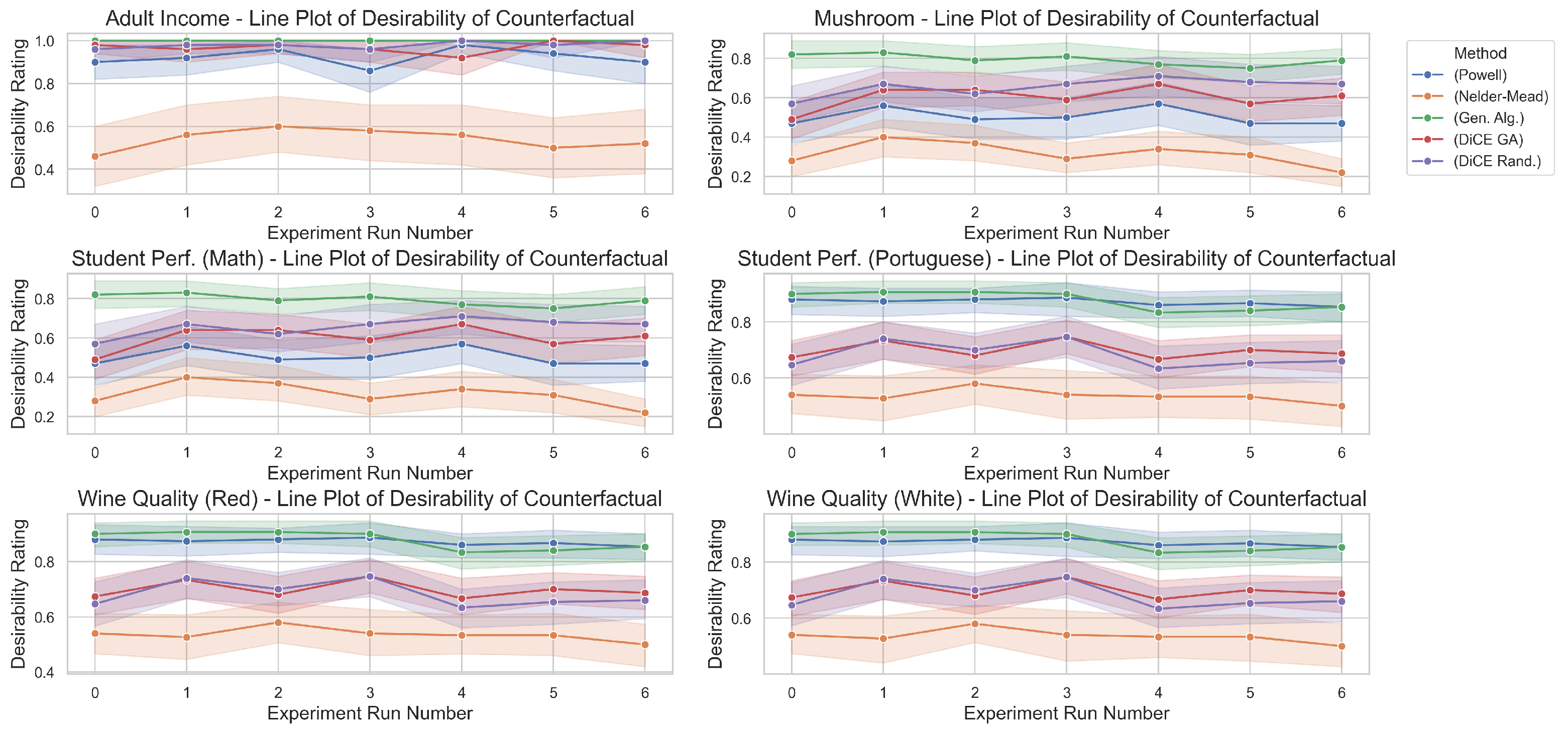
A key performance difference is shown in Figure 11, which displays the desirability ratings of the counterfactuals generated by the various methods. For the single-output binary classification problem (Adult Income dataset), all methods perform relatively well with a high rate of finding desired counterfactuals. However, this does not hold for datasets with higher output dimensions. In the case of the Wine Quality dataset (both red and white), the DiCE method performs below both our custom Genetic Algorithm and Powell’s method. A more significant issue arises with multi-output problems: DiCE lacks an inherent method for generating valid counterfactuals for multiple outputs simultaneously. To address this, we generated multiple counterfactuals for each output individually and selected the best overall counterfactual. As seen in the Student Performance and Mushroom datasets, the average desirability of the counterfactuals generated via DiCE remains between 0.4 and 0.6. In contrast, our custom Genetic Algorithm consistently produces highly desirable counterfactuals.
Table 3 presents a performance comparison of four different optimization methods employed to generate counterfactual explanations: Powell’s method, a custom Genetic Algorithm, a Genetic Algorithm implemented using the DiCE library, and Random Selection via DiCE. The table excludes the Nelder–Mead method, as it failed to generate desirable counterfactuals in most instances. The table summarizes the average distance between original and counterfactual inputs, the time required for optimization, and counterfactual desirability across three weighting schemes: equal weights, random weights, and a mixed objective function (which gives 95% weight to validity and 5% weight to distance). DiCE’s Genetic Algorithm demonstrated a reasonable balance between distance and time, whereas Powell’s method, while offering lower computation times than some methods, resulted in higher distances. Random selection consistently had the lowest average distances and times but lacked optimization toward counterfactual desirability. This performance deficit can be attributed to its inability to evaluate desirability for multiple outputs simultaneously. Optimization algorithms implementing the DeRaC framework consistently performed better in terms of overall counterfactual desirability, although an uncharacteristic underperformance was observed for the custom Genetic Algorithm during mixed-objective optimization. Overall, the results highlight trade-offs between solution accuracy, computational efficiency, and the ability to optimize for specific counterfactual characteristics.

Illustrative Case Study and Model Interpretation

To demonstrate the practical utility of the DeRaC framework for model analysis, we present a case study using the Student Performance (Portuguese) dataset. We consider a specific instance where the objective is to satisfy a complex, multi-output goal: achieving a target profile where the first two output dimensions are below average and the third is above average (targets [0,0,1] with randomly generated weights [8,10,3]).
The original instance is characterized by failures = 0, studytime = 2, famrel = 4, and absences = 0.
When applying the standard DiCE (Genetic Algorithm) method, the generated counterfactual attempts to reach the goal by perturbing a wide array of features, including studytime (from 2 to 1), famrel (from 4 to 2), goout (from 3 to 4.2), and Walc (from 1 to 4.2). Despite these multiple changes, the DiCE method only achieves a desirability rating of 0.381, failing to satisfy the multi-output target profile. From an interpretability standpoint, this provides a “noisy” explanation; the multitude of changes makes it difficult for a human user to discern which feature is actually driving the model’s decision.
In contrast, the DeRaC framework (utilizing Powell’s method) achieves a perfect desirability rating of 1.0. The counterfactual generated is far more surgical, primarily identifying that a change in failures (from 0 to 3) is the key driver to satisfy the complex multi-output target.
This comparison provides two critical insights for model analysis:
1.
Feature Sensitivity: DeRaC reveals that the model’s decision boundary for this specific multi-output goal is most sensitively tied to the failures feature.
2.
Explanation Clarity: Unlike the scattered perturbations in the DiCE method, DeRaC provides a clear, minimal set of changes. This allows a practitioner to conclude that according to the model, the target outcome is highly dependent on the student’s academic history (failures) rather than social factors like goout or Walc, thereby offering a much cleaner and more actionable interpretation of the model’s internal logic.

7. Discussion

This paper demonstrates the feasibility of systematically generating valid counterfactual explanations for classification problems with varying output space complexities, including single and multi-output classification tasks with both binary and multi-class outputs. The consistent ability to define and find counterfactuals across diverse datasets while maintaining model-agnosticism highlights the potential of this approach for eXplainable AI. The observed higher desirability ratings for counterfactual instances compared to original instances (Figure 9) demonstrate the ability to define and find valid counterfactuals using existing optimization methods. This is further supported by the percentage of partially or completely valid counterfactuals achieved, which varies across datasets and optimization methods (Figure 10). We also measured similarity, as defined by Guidotti [5], by assessing distance (Figure 11), which provides insight into how distinct the counterfactuals are from the original instances.
Our results emphasize the crucial role of defining the “desired output” in counterfactual generation, as this choice significantly impacts validity, proximity, and similarity. Different strategies for determining this desired output led to varying results in terms of desirability rating, distance, and the number of features changed even within the same dataset. This underlines the inherently case-dependent nature of counterfactual explanations, and it also highlights the ability to generate a diverse set of counterfactuals based on the sample and the desired output for that case. The lack of a universally “best” method for defining the desired output suggests that the optimal approach will be task-specific and potentially user-defined, especially in goal-achievement scenarios as discussed. In contrast, for model-analysis purposes, the desired output is typically instance-specific and less user-defined.
While we explicitly evaluated validity and similarity—as demonstrated by the feasibility of mixed objective functions in Table 3—other important properties of counterfactual explanations warrant further consideration. Properties such as plausibility, actionability and discriminative power need further analysis and empirical experiments. The observed differences in success rates across datasets between implementing DeRaC and existing counterfactual generation frameworks suggest that data distribution and model complexity significantly influence the effectiveness of counterfactual generation. Furthermore, the concept of diversity remains unaddressed; generating a single counterfactual may not fully capture the range of possible alternative outcomes, and future studies should explore the effects of different optimization methods on these different properties of a counterfactual.
This paper directly contributes to the growing field of eXplainable AI (XAI) by providing a robust and flexible framework, DeRaC, for generating instance-level explanations. By systematically perturbing input features to achieve a desired outcome, we can probe model sensitivities and identify crucial feature interactions [40]. For example, analyzing which features consistently change across counterfactuals for a particular class reveals potential biases or unexpected dependencies within the model. Furthermore, the metrics we employ, validity, similarity, and minimality, offer quantifiable insights into the quality of these explanations, allowing for a comparative analysis of different models or training procedures. This capability to assess explanation characteristics is essential for building trust and ensuring responsible AI development, enabling practitioners to not only understand what a model predicts, but also why it predicts it, and how easily that prediction could change [15].

Interpretability in Multi-Output Contexts

A critical aspect of explainability in complex tasks is understanding the interdependence of multiple outputs. As noted in our comparison with DiCE, standard methods often fail to maintain desirability across multiple dimensions simultaneously. Our results suggest that DeRaC provides a more holistic interpretation of multi-output models.
In datasets like Wine Quality (multi-class) or Student Performance (multi-output), a standard counterfactual might achieve a class change by perturbing a feature that negatively impacts a secondary desirable attribute. Because DeRaC optimizes for a context-dependent desirability rating, the generated explanations reveal the “trade-offs” the model makes between different output features. This allows users to see not just how to change a single prediction but also how various input features interact to drive multiple outputs toward a desired global state, providing a deeper layer of model transparency than single-output methods.

8. Conclusions

The aim of this paper is to formalize valid counterfactuals for all classification problems, including binary and multi-class classification, for both single and multi-output problems. Rather than changing existing definitions, the goal is to expand and codify them for problems that are not extensively discussed in the existing literature. Other works, such as [59], mention multi-class problems; however, they use the existing notion of any different classification as valid counterfactuals. As we discussed regarding the problems associated with this approach in Section 2, in case of multi-class and multi-output classification problems, simply a “different” classification is not always useful.
This problem was addressed by introducing the concept of a desirability rating, which depends on predefined context-dependent desired outputs. These desired outputs are not dependent on the dataset or the model but rather on the instance or the current use case (a concept that already exists in the counterfactual explanation literature [5]). We introduce the Desirability Rating-based Counterfactual (DeRaC) framework, demonstrating that it is possible to mathematically measure how desirable the original and the counterfactual instances are as well as the differences between them. A valid counterfactual is defined as a counterfactual instance with a desirability rating of 1, whereas any improvement from the original instance in desirability makes it at least partially valid. It can be thought of as being “on its way” to the desired output or “between” the original instance and the desired instance.
By expanding the definition of valid counterfactuals, we are still able to use concepts from earlier works, such as the properties of proximity, validity, similarity, and actionability [4,5]. In our experiments, we utilize existing optimization algorithms, including Powell’s method [65], the Nelder–Mead method [66], and Genetic Algorithm, as well as an implementation of the existing counterfactual generation library DiCE [6], to optimize for desirability rating (an expansion of existing validity property). We are able to generate counterfactuals based on different desired outputs for all datasets. These were tested on single-output binary classification, multi-class, and multi-output classification problems. The experiment was conducted by sampling the separate testing dataset with multiple runs for each method of selecting the desired output. These results demonstrate the reproducibility as well as the compatibility with various different desired outputs. This is particularly important given that complex multi-output classification problems have more than one possible desired output unlike single-output binary classification problems.
However, several avenues for future research remain. Testing on more datasets with combinations of multiple outputs and classes should give more weight to the proposed formalization. In future iterations, we can also test existing counterfactual generation methods, such as [31,34,39], that account for properties such as proximity, validity, similarity, and actionability on multi-class and multi-output problems. In the future, it is important to expand this formalization to regression problems and study their efficiency and computational cost. Finally, user studies are needed to assess the human interpretability and trustworthiness of these counterfactual explanations, ultimately determining their value in real-world applications like decision support, model debugging, and fairness auditing. This research lays the groundwork for building more transparent, understandable, and trustworthy machine learning systems.

Author Contributions

Conceptualization, N.K. and M.K.; methodology, N.K.; validation, N.K.; writing—original draft preparation, N.K.; writing—review and editing, N.K. and M.K.; supervision, M.K. All authors have read and agreed to the published version of the manuscript.

Funding

This research received no external funding.

Data Availability Statement

The datasets used in this study are publicly available and can be accessed from the repositories cited in the manuscript: The Mushroom dataset; The Student Performance dataset; The Wine dataset; The Adult Income dataset. No new primary data were collected in this study.

Conflicts of Interest

The authors declare no conflicts of interest.

References

  1. Cao, L. AI in finance: Challenges, techniques, and opportunities. ACM Comput. Surv. (CSUR) 2022, 55, 1–38. [Google Scholar]
  2. Goswami, G.; Bhardwaj, R.; Singh, R.; Vatsa, M. MDLFace: Memorability augmented deep learning for video face recognition. In IEEE International Joint Conference on Biometrics; IEEE: Piscataway, NJ, USA, 2014; pp. 1–7. [Google Scholar]
  3. Sarker, I.H.; Furhad, M.H.; Nowrozy, R. AI-driven cybersecurity: An overview, security intelligence modeling and research directions. SN Comput. Sci. 2021, 2, 173. [Google Scholar] [CrossRef]
  4. Verma, S.; Boonsanong, V.; Hoang, M.; Hines, K.E.; Dickerson, J.P.; Shah, C. Counterfactual Explanations and Algorithmic Recourses for Machine Learning: A Review. arXiv 2022, arXiv:2010.10596. [Google Scholar] [CrossRef]
  5. Guidotti, R. Counterfactual explanations and how to find them: Literature review and benchmarking. Data Min. Knowl. Discov. 2024, 38, 2770–2824. [Google Scholar] [CrossRef]
  6. Mothilal, R.K.; Sharma, A.; Tan, C. Explaining machine learning classifiers through diverse counterfactual explanations. In Proceedings of the 2020 Conference on Fairness, Accountability, and Transparency, Barcelona, Spain, 27–30 January 2020; pp. 607–617. [Google Scholar] [CrossRef]
  7. Fisher, R.A. Iris. UCI Machine Learning Repository. 1936. Available online: https://archive.ics.uci.edu/dataset/53/iris (accessed on 26 May 2025).
  8. Cortez, P.; Cerdeira, A.; Almeida, F.; Matos, T.; Reis, J. Wine Quality. UCI Machine Learning Repository. 2009. Available online: https://archive.ics.uci.edu/dataset/186/wine+quality (accessed on 26 May 2025).
  9. Marcinkevičs, R.; Vogt, J.E. Interpretable and explainable machine learning: A methods-centric overview with concrete examples. Wiley Interdiscip. Rev. Data Min. Knowl. Discov. 2023, 13, e1493. [Google Scholar] [CrossRef]
  10. Ali, S.; Abuhmed, T.; El-Sappagh, S.; Muhammad, K.; Alonso-Moral, J.M.; Confalonieri, R.; Guidotti, R.; Del Ser, J.; Díaz-Rodríguez, N.; Herrera, F. Explainable Artificial Intelligence (XAI): What we know and what is left to attain Trustworthy Artificial Intelligence. Inf. Fusion 2023, 99, 101805. [Google Scholar] [CrossRef]
  11. Džeroski, S.; Demšar, D.; Grbović, J. Predicting Chemical Parameters of River Water Quality from Bioindicator Data. Appl. Intell. 2000, 13, 7–17. [Google Scholar] [CrossRef]
  12. Li, H.; Zhang, W.; Chen, Y.; Guo, Y.; Li, G.Z.; Zhu, X. A novel multi-target regression framework for time-series prediction of drug efficacy. Sci. Rep. 2017, 7, 40652. [Google Scholar] [CrossRef] [PubMed]
  13. Borchani, H.; Varando, G.; Bielza, C.; Larrañaga, P. A survey on multi-output regression. WIREs Data Min. Knowl. Discov. 2015, 5, 216–233. [Google Scholar] [CrossRef]
  14. Xu, D.; Shi, Y.; Tsang, I.W.; Ong, Y.S.; Gong, C.; Shen, X. Survey on Multi-Output Learning. IEEE Trans. Neural Netw. Learn. Syst. 2020, 31, 2409–2429. [Google Scholar] [CrossRef]
  15. Wachter, S.; Mittelstadt, B.; Russell, C. Counterfactual Explanations without Opening the Black Box: Automated Decisions and the GDPR. Harv. J. Law Technol. (Harv. JOLT) 2017, 31, 841–888. [Google Scholar] [CrossRef]
  16. Bodria, F.; Giannotti, F.; Guidotti, R.; Naretto, F.; Pedreschi, D.; Rinzivillo, S. Benchmarking and survey of explanation methods for black box models. Data Min. Knowl. Discov. 2023, 37, 1719–1778. [Google Scholar] [CrossRef]
  17. Stepin, I.; Alonso, J.M.; Catala, A.; Pereira-Fariña, M. A survey of contrastive and counterfactual explanation generation methods for explainable artificial intelligence. IEEE Access 2021, 9, 11974–12001. [Google Scholar] [CrossRef]
  18. Keane, M.T.; Kenny, E.M.; Delaney, E.; Smyth, B. If Only We Had Better Counterfactual Explanations: Five Key Deficits to Rectify in the Evaluation of Counterfactual XAI Techniques. In Proceedings of the Thirtieth International Joint Conference on Artificial Intelligence, Montreal, QC, Canada, 16–22 August 2021; pp. 4466–4474. [Google Scholar] [CrossRef]
  19. Laugel, T.; Jeyasothy, A.; Lesot, M.J.; Marsala, C.; Detyniecki, M. Achieving diversity in counterfactual explanations: A review and discussion. In Proceedings of the 2023 ACM Conference on Fairness, Accountability, and Transparency, Chicago, IL, USA, 12–15 June 2023; pp. 1859–1869. [Google Scholar]
  20. Jiang, J.; Leofante, F.; Rago, A.; Toni, F. Robust counterfactual explanations in machine learning: A survey. arXiv 2024, arXiv:2402.01928. [Google Scholar] [CrossRef]
  21. Mertes, S.; Huber, T.; Weitz, K.; Heimerl, A.; André, E. Ganterfactual—Counterfactual explanations for medical non-experts using generative adversarial learning. Front. Artif. Intell. 2022, 5, 825565. [Google Scholar] [CrossRef]
  22. Del Ser, J.; Barredo-Arrieta, A.; Díaz-Rodríguez, N.; Herrera, F.; Saranti, A.; Holzinger, A. On generating trustworthy counterfactual explanations. Inf. Sci. 2024, 655, 119898. [Google Scholar] [CrossRef]
  23. Pawelczyk, M.; Agarwal, C.; Joshi, S.; Upadhyay, S.; Lakkaraju, H. Exploring counterfactual explanations through the lens of adversarial examples: A theoretical and empirical analysis. In Proceedings of the International Conference on Artificial Intelligence and Statistics, PMLR, Virtual, 28–30 March 2022; pp. 4574–4594. [Google Scholar]
  24. Maaroof, N.; Moreno, A.; Valls, A.; Jabreel, M.; Romero-Aroca, P. Multi-Class Fuzzy-LORE: A Method for Extracting Local and Counterfactual Explanations Using Fuzzy Decision Trees. Electronics 2023, 12, 2215. [Google Scholar] [CrossRef]
  25. Dastile, X.; Celik, T. Counterfactual explanations with multiple properties in credit scoring. IEEE Access 2024, 12, 110713–110728. [Google Scholar] [CrossRef]
  26. Prado-Romero, M.A.; Prenkaj, B.; Stilo, G.; Celi, A.; Estevanell-Valladares, E.L.; Pérez, D.A.V. Ensemble Approaches for Graph Counterfactual Explanations. In CEUR Workshop Proceedings; RWTH Aachen University: Aachen, Germany, 2022; pp. 88–97. [Google Scholar]
  27. De Toni, G.; Lepri, B.; Passerini, A. Synthesizing explainable counterfactual policies for algorithmic recourse with program synthesis. Mach. Learn. 2023, 112, 1389–1409. [Google Scholar] [CrossRef]
  28. Kanamori, K.; Takagi, T.; Kobayashi, K.; Ike, Y.; Uemura, K.; Arimura, H. Ordered counterfactual explanation by mixed-integer linear optimization. In Proceedings of the AAAI Conference on Artificial Intelligence, Virtual, 2–9 February 2021; Volume 35, pp. 11564–11574. [Google Scholar]
  29. Maiti, A.; Plecko, D.; Bareinboim, E. Counterfactual Identification Under Monotonicity Constraints. In Proceedings of the AAAI Conference on Artificial Intelligence, Philadelphia, PA, USA, 25 February–4 March 2025; Volume 39, pp. 26841–26850. [Google Scholar]
  30. Zhou, G.; Yao, L.; Xu, X.; Wang, C.; Zhu, L. Learning to infer counterfactuals: Meta-learning for estimating multiple imbalanced treatment effects. arXiv 2022, arXiv:2208.06748. [Google Scholar] [CrossRef]
  31. Cheng, F.; Ming, Y.; Qu, H. DECE: Decision Explorer with Counterfactual Explanations for Machine Learning Models. IEEE Trans. Vis. Comput. Graph. 2021, 27, 1438–1447. [Google Scholar] [CrossRef] [PubMed]
  32. Oprea, S.V.; Bâra, A. Customer-centric decision-making with XAI and counterfactual explanations for churn mitigation. J. Theor. Appl. Electron. Commer. Res. 2025, 20, 129. [Google Scholar] [CrossRef]
  33. Oprea, S.V.; Bâra, A. Diverse counterfactual explanations (DiCE) role in improving sales and e-commerce strategies. J. Theor. Appl. Electron. Commer. Res. 2025, 20, 96. [Google Scholar] [CrossRef]
  34. Wexler, J.; Pushkarna, M.; Bolukbasi, T.; Wattenberg, M.; Viegas, F.; Wilson, J. The What-If Tool: Interactive Probing of Machine Learning Models. IEEE Trans. Vis. Comput. Graph. 2019, 26, 26–65. [Google Scholar] [CrossRef]
  35. Tenney, I.; Wexler, J.; Bastings, J.; Bolukbasi, T.; Coenen, A.; Gehrmann, S.; Jiang, E.; Pushkarna, M.; Radebaugh, C.; Reif, E.; et al. The language interpretability tool: Extensible, interactive visualizations and analysis for NLP models. arXiv 2020, arXiv:2008.05122. [Google Scholar] [CrossRef]
  36. Krause, J.; Perer, A.; Ng, K. Interacting with Predictions: Visual Inspection of Black-box Machine Learning Models. In Proceedings of the 2016 CHI Conference on Human Factors in Computing Systems, San Jose, CA, USA, 7–12 May 2016; pp. 5686–5697. [Google Scholar] [CrossRef]
  37. Ming, Y.; Qu, H.; Bertini, E. RuleMatrix: Visualizing and Understanding Classifiers with Rules. IEEE Trans. Vis. Comput. Graph. 2019, 25, 342–352. [Google Scholar] [CrossRef]
  38. Gathani, S.; Hulsebos, M.; Gale, J.; Haas, P.J.; Demiralp, Ç. Augmenting decision making via interactive what-if analysis. arXiv 2021, arXiv:2109.06160. [Google Scholar]
  39. Gomez, O.; Holter, S.; Yuan, J.; Bertini, E. ViCE: Visual counterfactual explanations for machine learning models. In Proceedings of the 25th International Conference on Intelligent User Interfaces, Cagliari, Italy, 17–20 March 2020; pp. 531–535. [Google Scholar] [CrossRef]
  40. Kshetry, N.; Kantardzic, M. What-if XAI framework (WiXAI): From counterfactuals towards causal understanding. J. Comput. Commun. 2024, 12, 169–198. [Google Scholar] [CrossRef]
  41. Goyal, Y.; Wu, Z.; Ernst, J.; Batra, D.; Parikh, D.; Lee, S. Counterfactual visual explanations. In Proceedings of the International Conference on Machine Learning, PMLR, Long Beach, CA, USA, 9–15 June 2019; pp. 2376–2384. [Google Scholar]
  42. Kenny, E.M.; Delaney, E.D.; Greene, D.; Keane, M.T. Post-hoc explanation options for xai in deep learning: The insight centre for data analytics perspective. In International Conference on Pattern Recognition; Springer: Cham, Switzerland, 2021; pp. 20–34. [Google Scholar]
  43. Akula, A.R.; Wang, K.; Liu, C.; Saba-Sadiya, S.; Lu, H.; Todorovic, S.; Chai, J.; Zhu, S.C. CX-ToM: Counterfactual explanations with theory-of-mind for enhancing human trust in image recognition models. iScience 2022, 25, 103581. [Google Scholar] [CrossRef] [PubMed]
  44. Kenny, E.M.; Keane, M.T. On generating plausible counterfactual and semi-factual explanations for deep learning. In Proceedings of the AAAI Conference on Artificial Intelligence, Virtual, 2–9 February 2021; Volume 35, pp. 11575–11585. [Google Scholar]
  45. Thiagarajan, J.J.; Thopalli, K.; Rajan, D.; Turaga, P. Training calibration-based counterfactual explainers for deep learning models in medical image analysis. Sci. Rep. 2022, 12, 597. [Google Scholar] [CrossRef]
  46. Alipour, K.; Lahiri, A.; Adeli, E.; Salimi, B.; Pazzani, M. Explaining image classifiers using contrastive counterfactuals in generative latent spaces. arXiv 2022, arXiv:2206.05257. [Google Scholar] [CrossRef]
  47. Zhao, W.; Oyama, S.; Kurihara, M. Generating natural counterfactual visual explanations. In Proceedings of the Twenty-Ninth International Conference on International Joint Conferences on Artificial Intelligence, Yokohama, Japan, 7–15 January 2021; pp. 5204–5205. [Google Scholar]
  48. Robeer, M.; Bex, F.; Feelders, A. Generating realistic natural language counterfactuals. In Findings of the Association for Computational Linguistics: EMNLP 2021; Association for Computational Linguistics: Stroudsburg, PA, USA, 2021; pp. 3611–3625. [Google Scholar]
  49. Arie, A.B.; Deutch, D.; Frost, N.; Horesh, Y.; Meyuhas, I. Optimizing Counterfactual-based Analysis of Machine Learning Models Through Databases. In Proceedings of the 27th International Conference on Extending Database Technology, EDBT 2024, Paestum, Italy, 25–28 March 2024; pp. 597–609. [Google Scholar]
  50. Piccialli, V.; Morales, D.R.; Salvatore, C. Supervised feature compression based on counterfactual analysis. Eur. J. Oper. Res. 2024, 317, 273–285. [Google Scholar] [CrossRef]
  51. Artelt, A.; Gregoriades, A. “How to make them stay?”—Diverse Counterfactual Explanations of Employee Attrition. arXiv 2023, arXiv:2303.04579. [Google Scholar]
  52. Gao, R.; Biggs, M.; Sun, W.; Han, L. Enhancing counterfactual classification via self-training. arXiv 2021, arXiv:2112.04461. [Google Scholar] [CrossRef]
  53. Temraz, M.; Keane, M.T. Solving the class imbalance problem using a counterfactual method for data augmentation. Mach. Learn. Appl. 2022, 9, 100375. [Google Scholar] [CrossRef]
  54. Sohns, J.T.; Garth, C.; Leitte, H. Decision boundary visualization for counterfactual reasoning. In Computer Graphics Forum; Wiley Online Library: Hoboken, NJ, USA, 2023; Volume 42, pp. 7–20. [Google Scholar]
  55. Mahajan, D.; Tan, C.; Sharma, A. Preserving causal constraints in counterfactual explanations for machine learning classifiers. arXiv 2019, arXiv:1912.03277. [Google Scholar]
  56. Duong, T.D.; Li, Q.; Xu, G. Causality-based counterfactual explanation for classification models. Knowl.-Based Syst. 2024, 300, 112200. [Google Scholar] [CrossRef]
  57. Xia, K.; Pan, Y.; Bareinboim, E. Neural causal models for counterfactual identification and estimation. arXiv 2022, arXiv:2210.00035. [Google Scholar] [CrossRef]
  58. Crupi, R.; González, B.S.M.; Castelnovo, A.; Regoli, D. Leveraging Causal Relations to Provide Counterfactual Explanations and Feasible Recommendations to End Users. In Proceedings of the 14th International Conference on Agents and Artificial Intelligenc ICAART (2); SCITEPRESS—Science and Technology Publications: Setúbal, Portugal, 2022; pp. 24–32. [Google Scholar]
  59. Carlevaro, A.; Lenatti, M.; Paglialonga, A.; Mongelli, M. MultiClass Counterfactual Explanations using Support Vector Data Description. IEEE Trans. Artif. Intell. 2023, 5, 3046–3056. [Google Scholar] [CrossRef]
  60. Caron, A.; Baio, G.; Manolopoulou, I. Counterfactual Learning with Multioutput Deep Kernels. arXiv 2022, arXiv:2211.11119. [Google Scholar] [CrossRef]
  61. Parbhoo, S.; Bauer, S.; Schwab, P. Ncore: Neural counterfactual representation learning for combinations of treatments. arXiv 2021, arXiv:2103.11175. [Google Scholar] [CrossRef]
  62. Mushroom. UCI Machine Learning Repository. 1981. Available online: https://archive.ics.uci.edu/dataset/73/mushroom (accessed on 26 May 2025).
  63. Cortez, P. Student Performance. UCI Machine Learning Repository. 2008. Available online: https://archive.ics.uci.edu/dataset/320/student+performance (accessed on 26 May 2025).
  64. Becker, B.; Kohavi, R. Adult. UCI Machine Learning Repository. 1996. Available online: https://archive.ics.uci.edu/dataset/2/adult (accessed on 26 May 2025).
  65. Powell, M.J.D. An efficient method for finding the minimum of a function of several variables without calculating derivatives. Comput. J. 1964, 7, 155–162. [Google Scholar] [CrossRef]
  66. Gao, F.; Han, L. Implementing the Nelder-Mead simplex algorithm with adaptive parameters. Comput. Optim. Appl. 2012, 51, 259–277. [Google Scholar] [CrossRef]
  67. Virtanen, P.; Gommers, R.; Oliphant, T.E.; Haberland, M.; Reddy, T.; Cournapeau, D.; Burovski, E.; Peterson, P.; Weckesser, W.; Bright, J.; et al. SciPy 1.0: Fundamental Algorithms for Scientific Computing in Python. Nat. Methods 2020, 17, 261–272. [Google Scholar] [CrossRef] [PubMed]
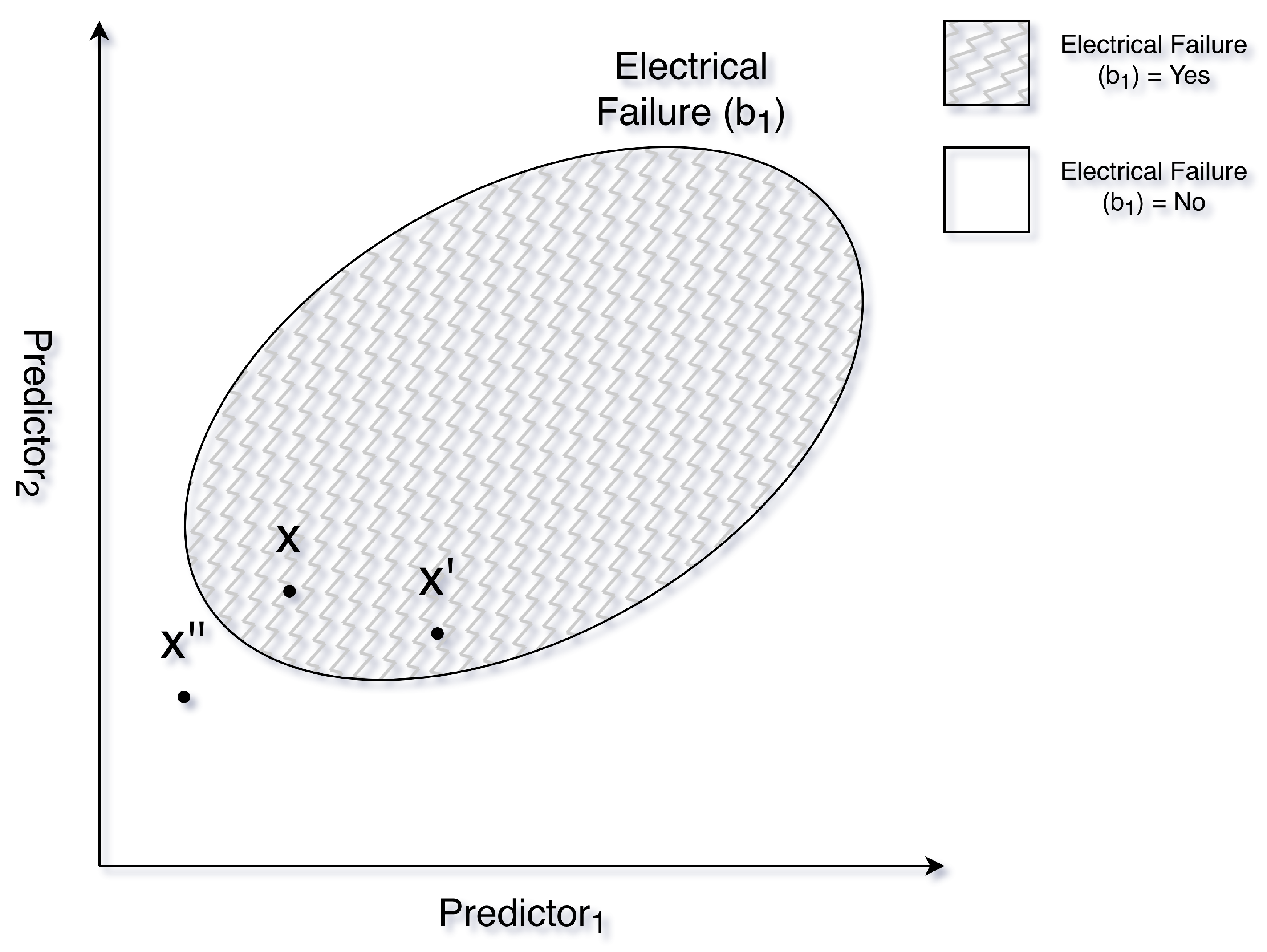
Figure 1. Example of valid and invalid counterfactual instance x′ and x″ based on original instance x and classification model b1.
Make 08 00109 g001
Figure 2. Classification for multi-class (3 classes) problem where the classes are c0, c1, and c2.
Make 08 00109 g002
Figure 3. Two-output binary classification problem where outputs o1, o2 are modeled by b1, b2 each giving either a Yes or No class.
Make 08 00109 g003
Figure 4. A schema of the experiment setup using 50 random samples for each of the six datasets (from four data sources) repeated for seven runs.
Make 08 00109 g004
Figure 5. Boxplot of original desirability for all datasets with the red line indicating the average.
Make 08 00109 g005
Figure 6. Boxplot of CF desirability for Student Performance (Math) dataset with the red line indicating the average.
Make 08 00109 g006
Figure 7. Boxplot of difference in desirability for each dataset, with the red line indicating the average, showing a systematic generation of valid counterfactuals.
Make 08 00109 g007
Figure 8. Barplot of portion of valid and partially valid counterfactuals found with different methods.
Make 08 00109 g008
Figure 9. Average distance of counterfactual instance from original instance for each run of experiment for the different methods of counterfactual generation.
Make 08 00109 g009
Figure 10. Average time to find counterfactual solution for different methods across all the dataset for the different runs of the experiment.
Make 08 00109 g010
Figure 11. Desirability Rating of the counterfactuals generated by the different methods for all datasets across the various different experiment runs.
Make 08 00109 g011
Table 1. Desirable properties of counterfactual explanations [5].
PropertyDescription
ValidityA counterfactual x is valid if it changes the classification outcome: b ( x ) b ( x ) .
Minimality (Sparsity) x is minimal if it has the fewest attribute changes compared to other valid counterfactuals x .
Similarity (Proximity) x should be close to x based on a distance function d: d ( x , x ) < ϵ , where ϵ is a predefined threshold. This is also referred to as proximity.
Plausibility x should have feature values consistent with a reference population X. Values should be realistic and not outliers within X. This is also known as feasibility or reliability.
Discriminative Power x should clearly demonstrate the reasons for the change in prediction. A human observing x and x should understand the differing classification.
Actionability x should only differ from x in terms of actionable features (features that can be changed). Immutable features should remain constant. This is also known as recourse.
Causality x should respect known causal relationships between features, as defined by a Directed Acyclic Graph (DAG). Changes in features should maintain established causal links.
DiversityA set of counterfactuals C = { x 1 , , x h } should be diverse, maximizing the difference between the counterfactuals while maintaining minimality and similarity.
Table 2. Summary of datasets used in the experiments.
Dataset NameDescriptionOutput Type/ProblemNumber of OutputsKey Features
Mushroom
Dataset [62]
Classifies mushrooms as edible or poisonous based on 22 features.Categorical, Multi-class Classification (Edible/Poisonous + Habitat)222 Features
Student Performance
Dataset [63]
Information about students’ performance in secondary school (grades, demographics).Binary Classification (Above/Below Average)3 (First, Second, Final Period)Grades in First, Second, and Final Periods, Demographic Features
Wine Dataset [8]Chemical properties of wines and a quality rating.Ordinal Multi-class Classification1Chemical Properties
Adult Income Dataset [64]Demographic features of individuals.Binary Classification (Income > or <$50K/year)1Education, Age, Marital Status, etc.
Note: The Wine and Student Performance datasets are treated as two separate problems (Red Wine & White Wine and Math & Portuguese, respectively).
Table 3. Performance comparison of different optimization methods for counterfactual generation.
MetricsPowell’s MethodGenetic AlgorithmDiCE (GA)DiCE (Rand.)
Distance (Equal Weights)7.3984.1182.5510.909
Distance (Random Weights)7.5144.0952.6110.979
Distance (Mixed Objective)0.8971.8642.5360.878
Time in Milliseconds (Equal Weights)1358.969479.89444.963758.152
Time in Milliseconds (Random Weights)2246.62715,851.816603.4811694.52
Time in Milliseconds (Mixed Objective)1178.4482217.728328.514979.416
CF Desirability (Equal Weights)0.8720.8770.6980.683
CF Desirability (Random Weights)0.8510.9120.7190.708
CF Desirability (Mixed Objective)0.8890.8050.7290.694
Disclaimer/Publisher’s Note: The statements, opinions and data contained in all publications are solely those of the individual author(s) and contributor(s) and not of MDPI and/or the editor(s). MDPI and/or the editor(s) disclaim responsibility for any injury to people or property resulting from any ideas, methods, instructions or products referred to in the content.