Article

Deep Learning-Based Synthesis, Classification and Analysis of Sedimentation Boundaries in Analytical Centrifugation Experiments


1
Institute of Interfaces and Particle Technology, Friedrich-Alexander-Universität, Erlangen-Nürnberg, 91058 Erlangen, Germany
2
LUM GmbH, 12489 Berlin, Germany
3
Institute of Mechanical Process Engineering and Mechanics (MVM), Karlsruhe Institute of Technology (KIT), 76131 Karlsruhe, Germany
4
Intelligent Systems Group (IS), Faculty of Computer Science, University of Duisburg-Essen (UDE), 47057 Duisburg, Germany
*
Author to whom correspondence should be addressed.
These authors contributed equally to this work.
Mach. Learn. Knowl. Extr. 2026, 8(3), 81; https://doi.org/10.3390/make8030081
Submission received: 27 January 2026 / Revised: 3 March 2026 / Accepted: 11 March 2026 / Published: 20 March 2026

Abstract

Applications for machine learning (ML) and deep learning (DL) are constantly growing and have already been adopted in the field of particle measurement technology. Even though analytical (ultra-)centrifugation (AC/AUC) is a widely used technique for characterizing dispersed particle systems, ML and DL have not yet been applied in this area. Data evaluation and interpretation in AC/AUC can be challenging and often requires expert knowledge. DL models can help, but their development is limited by a lack of annotated training data. One solution is to generate and use synthetic data instead. In the first part of this study, a model was trained to synthesize data from experiments using a combination of Variational Autoencoder (VAE) and Generative Adversarial Networks (GANs). The results appear highly realistic. Novice users could distinguish real from synthetic samples with only 63% accuracy. Then, a classifier was trained on experimental AC data to categorize real-world examples based on their underlying separation kinetics, testing different DL architectures. After initial training, the models were further fine-tuned with synthetic AC data. ResNet34 models achieved the best performance with 94% accuracy, comparable to an AC expert (91%), while inexperienced users reached only 53%. In the second part of our study, a regression model was trained for the analysis of sedimentation coefficients. Therefore, various generative models were developed and evaluated for synthesizing AUC data based on numerically simulated sedimentation boundaries. The best results were achieved by combining VAE and GAN architectures with embedded physical constraints. However, the generative networks have so far led to additional smearing of the profiles, resulting in a broadening of the sedimentation coefficient distribution and indicating that further refinement is necessary.

1. Introduction

Machine learning- and data-driven methodologies are becoming increasingly significant in various domains of research and innovation, such as emergency management [1], solvent chemistry [2], microalgae cultivation [3], tumor detection [4], text and language processing [5,6], and image analysis [7,8,9]. In recent years, significant advancements in deep learning (DL) architectures, coupled with the increased availability of computational power, have enabled a broader range of interdisciplinary applications [10,11]. This includes the integration of DL into particle technology for use in areas such as polymer characterization [12], biopharmaceutical particles [13], nanoparticles morphologies [14] and airborne particle sensors [15]. Recent research topics predominantly emphasize image-based particle characterization [16]. In particular, deriving size distributions from microscopic images can be time-consuming. Consequently, a widely employed application involves leveraging DL architectures for the automated segmentation [17], analysis of size and shape of nanoparticles based on scanning electron microscope images [18], transmission electron microscopy [19], or quantification of size and refractive index based on holographic images [20]. As the performance of DL architectures often depends on the amount of available annotated training data, which is often limited for particle images, research is increasingly focusing on generating synthetic particle images for use in training neural networks [21,22,23].
In addition to imaging techniques, many other measurement techniques are used for particle characterization, such as dynamic light scattering, static light scattering, laser diffraction, single particle scattering, or separation methods. Among these, analytical centrifugation (AC) [24] and analytical ultracentrifugation (AUC) [25] have emerged as a powerful absolute measurement techniques because they detect the transport properties of suspended particles in a liquid as a function of time and with high spatial resolution by tracking the sedimentation boundaries directly within the centrifugal field. AC is a table-top centrifuge with the capacity of measuring 12 samples at maximum rotor speed of 4000 rotation per minute, simultaneously. AC is often used to analyze the stability of suspensions and emulsions [26]. In the literature, AC measurement data are typically reported as transmission values over the radial position, with the time evolution color-coded from red to green [27]. Because of its specification, AC is particularly suited for larger colloids, complex formulations, and concentrated systems. The separation behavior can be classified mainly based on sedimentation or flotation, as well as mixtures thereof and non-ideality effects such as flocculation and aggregation at high concentrations [28,29]. However, despite the numerous applications of AC, still a manual workflow is used for data evaluation, which can be challenging for less experienced users. For several analysis methods, it is necessary to classify the separation behavior beforehand in order to select an appropriate calculation algorithm. Additionally, the experimenter must ensure that the analysis parameters are correctly set for the intended quantitative analysis. Classifying separation kinetics can vary in complexity depending on the system under investigation and typically requires a certain level of expertise. A data-driven algorithm can potentially mimic this expertise, making the process more accessible for less experienced users.
The AUC extends these capabilities to much smaller size scales, and it is considered the gold standard for characterizing particles and macromolecules. Operating under vacuum, AUC provides very stable temperature control during measurement. The maximum rotor speed can be increased to 60,000 rotations per minute while measuring four samples simultaneously. Furthermore, depending on the application, different optical sensors can be equipped, such as multi-wavelength [30], interference or emission detectors [31]. Sedimentation velocity experiments carried out using AUC are effective methods for characterizing dispersed systems. In particular, they can be used to analyze nanoparticles and particle systems with different particle size distributions with a high degree of precision [32]. AUC can also be used to analyze the composition of alloy nanoparticles [33], core-shell nanoparticles [34], and even for the multidimensional analysis of nanotubes [30], nanorods [35], and bipyramids [36]. Furthermore, the separation process is well understood and can be simulated using numerical methods [37,38]. In AUC the transport behavior is expressed in terms of the apparent, not diffusion corrected, sedimentation coefficient, which describes the settling velocity in a given centrifugal field. Although numerical solvers can be employed for this purpose, they require the meniscus position to be clearly identifiable within the dataset [37].
For automation, a sufficiently large and representative training dataset is essential to develop data-driven classification and regression models. To overcome the limitations of available annotated experimental data, an approach involving synthesized data can be used. Generative Adversarial Networks (GANs) and Variational Autoencoders (VAEs) are two types of network commonly used for artificially generating a wide variety of images [39,40,41]. As both types of networks have their respective strengths and weaknesses, hybrid architectures have been developed to enhance image synthesis. One area of application is medical diagnostics, where synthesized data is used to overcome the limitation of insufficient training data [42,43]. We have therefore also developed hybrid neural networks to synthesize new AC/AUC data.
In this work, we address the automation of sedimentation data analysis in AC experiments using DL approaches trained on real and synthetically generated data. The workflow is structured sequentially. First, AC transmission profiles are classified according to their separation kinetics (sedimentation, flotation, mixed behavior, and invalid measurements). This classification step serves as a prerequisite for further quantitative analysis. In the second step, data-driven regression models are developed to estimate apparent sedimentation coefficients from simulated AUC data. To compensate for limited annotated datasets, hybrid generative neural networks are developed to synthesize physically plausible AC and AUC profiles, which are used to augment model training. The generated data are evaluated qualitatively via expert user assessment and quantitatively through classification and regression performance metrics. This study focuses exclusively on data-driven methods for post-measurement analysis and does not address physics-based inverse modeling. Although this study has focused on model systems that are almost monodisperse and predominantly monomodal, our work aims to lay the foundation for future research into advanced tools that support the analysis and prediction of more complex, polydisperse and multimodal systems.

2. Theoretical Background

2.1. Separation Kinetics in Analytical Centrifugation

Particle or dispersion characterization can be achieved using sedimentation techniques such as AC [27]. An AC is a tabletop centrifuge equipped with a multi-sample rotor, where liquid-based dispersions are loaded into disposable rectangular cells and positioned horizontally. A collimated LED light beam passes through the sample, and a line detector array (spatial resolution of 14 µm) records the transmitted intensity at different time stages during centrifugation (see Figure 1).
Particles within the dispersion obstruct light, while particle-free regions allow for almost complete transmission, creating a spatially resolved optical extinction gradient over time. A simple formulation for the relationship between transmission and moderate particulate concentration follows the Lambert–Beer law in Equation (1):
log 10 ( T ) = log 10 ( I / I 0 ) = ε l c
where T is the transmission, I is the transmitted intensity, I 0 is the reference intensity of the measurement cell filled with the continuous phase only. ε is the extinction coefficient, l the sample path length and c the particle concentration.
Particles dispersed in a liquid can move to the cell bottom (sedimentation) or the meniscus (flotation) depending on the particle density relative to liquid density. In addition, mixed classes exist, referred to as suspoemulsions. Real-world samples often contain multiple dispersed phases with varying properties, including size distribution, density distribution, multimodality, and polydispersity. These samples may also exhibit non-ideal settling behaviors, such as flocculation, aggregation or hindered sedimentation/flotation, leading to a complex separation kinetics. These mechanisms add an additional time dependent settling behavior, called non-idealities. Classification helps to understand the behavior of the dispersed phase during centrifugation. Traditionally, classification relies on the expertise of the experimenter, sometimes introducing subjectivity. However, accurate identification of kinetic classes is crucial for selecting appropriate analytical methods for further analysis.

2.2. Fundamentals of Sedimentation Under Centrifugation

Particle move in a liquid under a gravitational or centrifugal field. Such movement is described by a balance of forces comprising the gravitational or centrifugal force as well as the buoyant force and drag force both acting in opposite direction. The balance of forces defines the direction and velocity of the particle’s movement and is defined in a centrifugation experiment as follows [44]:
F c e n t r i f u g a l + F b u o y a n c y + F d r a g = ( m p m s ) · ω 2 r f v = 0
where m p and m s are the mass of the particle and displaced solvent, respectively, ω is the angular velocity of the rotor, r is the distance from the center of rotation, f is the translational frictional coefficient which depends on the shape of the particle, and v is the sedimentation velocity. As the sedimentation velocity scales with the radial position, it can be related to the centrifugal acceleration providing the sedimentation coefficient s, which is defined as follows:
s = v ω 2 r
The sedimentation coefficient is given in units of Sved, where 1 Sved equals 10 13 s. Depending on the density difference between the particle and the surrounding medium, sedimentation, neutral buoyancy or flotation can occur. In terms of a centrifugation experiment, for sedimentation the particles will move radially outwards from the center of rotation (positive sedimentation coefficient), while for flotation the direction of movement is reversed (negative sedimentation coefficient) [44].
Due to the movement of the particles, a concentration gradient is formed within the measurement cell during an experiment. The change in concentration c over time t is described by a mass conservation approach, referred to as the Lamm equation for a sector-shaped centrifuge cell, taking into account local fluxes by sedimentation and diffusion:
c t = D 2 c r 2 + 1 r c r diffusion ω 2 s r c r + 2 c sedimentation
where D is the diffusion coefficient. While there exists no explicit full analytical solution, numerical algorithms can solve the Lamm equation accurately [45]. For particles larger than typically 20 nm, the effect of diffusion is quite small and therefore becomes negligible compared to sedimentation. In such cases, analytical solutions exist for the reduced Lamm equation (see Section 2.3). Based on the Stokes-Einstein relation, it is possible to calculate the size x of a sphere with equivalent sedimentation properties:
x = 18 η s ρ p ρ s
The viscosity of the solvent is η and the density of the particle is ρ p and the density of the surrounding media is ρ s .

2.3. Numerical Simulation of Sedimentation Boundaries

For a single and non-diffusing particle, the sedimentation profile can be calculated from the position-dependent velocity:
d r d t = s ω 2 r
which has the following solution:
r ( t ) = r 0 e s ω 2 t
r 0 describes the position of the particle at t = 0 s. For sedimentation, r 0 is described as the position of the meniscus formed at the liquid-air interface of the measurement volume. For flotation, r 0 is the bottom of the measurement cell. The concentration profile of a certain particle size can be described by a step function U ( s , r , t ) , which, for uniformly distributed non-interacting particles and neglecting diffusion effects in a sector-shaped cell, is defined as
U ( s , r , t ) = e 2 s ω 2 t × 0 for r < r 0 e s ω 2 t 1 else
Using this simplified function allows for the model to be easily extended to other cell geometries. For example, the sedimentation behavior in rectangular cells can be described with a modified step function [32]:
U ( s , r , t ) = e s ω 2 t × 0 for r < r 0 e s ω 2 t 1 else
Knowing the optical properties of the particles allows for the concentration profiles to be converted into extinction or transmission data. Furthermore, a set of experimental sedimentation velocity profiles a ( r , t ) can be described by the apparent sedimentation coefficient distribution g * ( s ) using the following equation:
a ( r , t ) g * ( s ) U ( s , r , t ) d s
To obtain the diffusion-corrected sedimentation coefficient distribution for small nanoparticles, the step function U ( s , r , t ) needs to be replaced by the solution of Lamm’s equation L ( s , D , r , t ) , which also takes the diffusion coefficient into account [37].

2.4. Generative Adversarial Networks

A GAN is a framework composed of two competing neural networks: a generator G and a discriminator D [46]. The generator learns to map random noise to samples that resemble real data, thereby synthesizing new data instances. At the same time, the discriminator estimates the probability that a given input is real (i.e., sampled from the training data distribution) or fake (i.e., generated by G). The training process of a GAN framework can be viewed as a two-player minimax game in which both networks iteratively improve over time through adversarial training. As the discriminator becomes increasingly better at distinguishing between real and fake samples, the generator, using feedback from the discriminator, improves its ability to produce realistic synthetic samples that can successfully fool the discriminator or adversary. The objective function for training a GAN is formally defined as follows:
G * , D * = arg   min G   max D   L G A N ( G , D )
where G * and D * denote the optimal states of the generator and discriminator, respectively. The function L G A N ( G , D ) represents the corresponding loss function, which is minimized with respect to G and maximized with respect to D. It is defined as
L G A N ( G , D ) = E X p d a t a ( X ) log D ( X ) + E z p z ( z ) log ( 1 D ( G ( z ) ) )
where E denotes the expected logarithmic probability assigned by the discriminator. The first term corresponds to a real sample X, drawn from the data distribution p d a t a ( X ) , while the second term relates to a synthetic sample generated by G from a noise vector z, sampled from a prior distribution p z ( z ) , typically a standard normal distribution. The discriminator learns to maximize this loss by assigning high probabilities to real samples X and low probabilities to fake samples G ( z ) . In contrast, only the second term is relevant when updating the generator. To minimize log ( 1 D ( G ( z ) ) ) , the generator must produce fake samples that closely resemble real data, thereby forcing the discriminator to assign them higher probabilities.
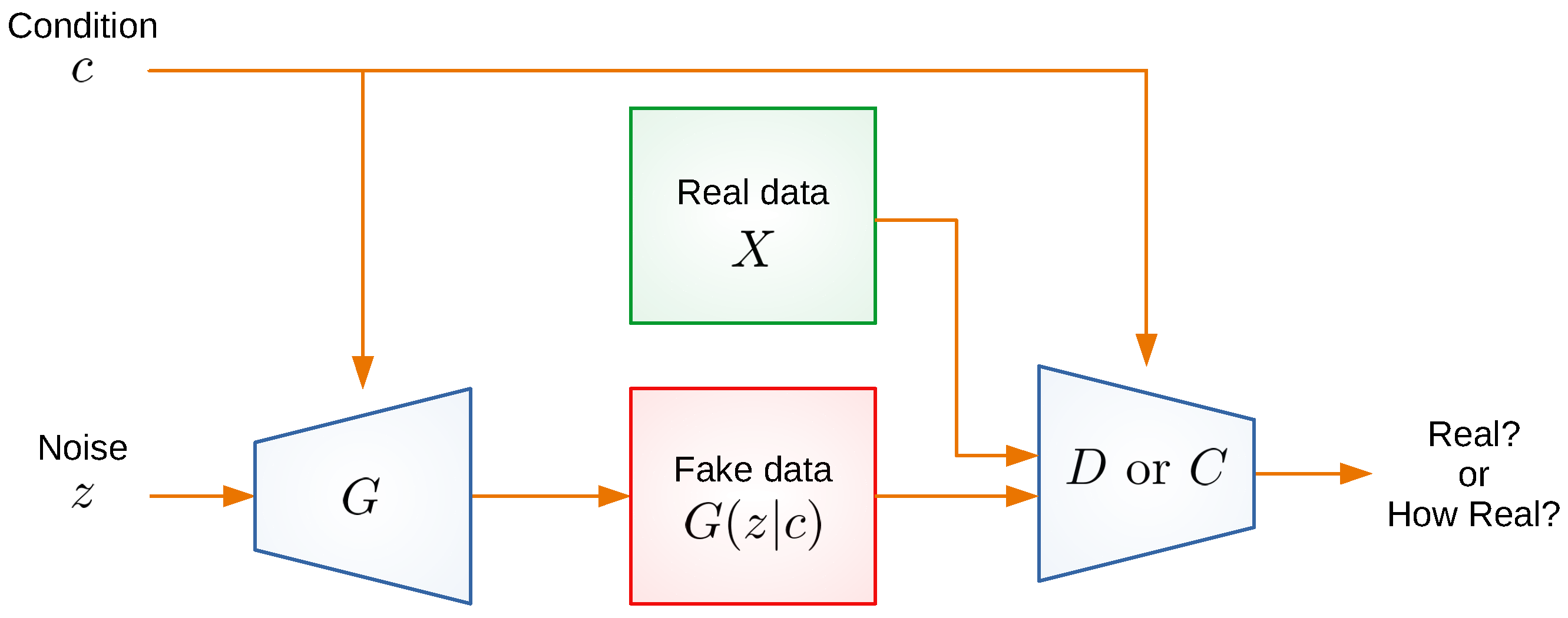
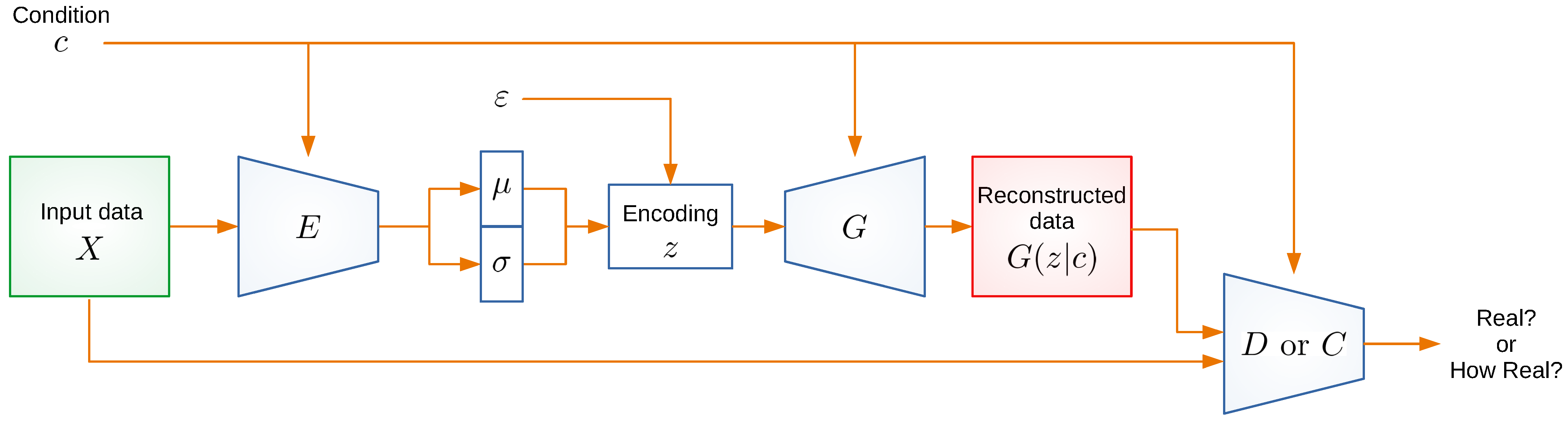
While standard GAN frameworks, such as Deep Convolutional GANs [47], allow for generating new data instances, they lack control over the characteristics of the output, making it challenging to guide the synthesis process. To address this limitation, the conditional GAN (cGAN) framework was proposed [48]. The cGAN framework incorporates auxiliary information, also referred to as a conditional prior, which is provided as an additional input to both the generator and the discriminator. The objective function for a cGAN closely resembles that of the standard GAN in Equation (12) and is defined as follows:
L c G A N ( G , D ) = E ( X , c ) p d a t a ( X , c ) log D ( X | c ) + E z p z ( z ) , c p d a t a ( c ) log ( 1 D ( G ( z | c ) | c ) )
where c denotes a conditional input, such as class labels, attributes, or other information. Although GANs have been widely used across various domains [49,50,51], they often suffer from issues such as mode collapse and training instability. These issues can hinder convergence and the diversity of generated outputs. Wasserstein GAN (WGAN) addresses these limitations by replacing the Jensen-Shannon divergence, used in standard GANs, with the Earth-Mover distance. This results in improved training stability, smoother gradients, fewer mode collapses, and a more interpretable loss [52]. The modified objective function for a conditional WGAN (cWGAN) can be defined as follows:
G * , C * = arg   min G   max C   L c W G A N ( G , C )
L c W G A N ( G , C ) = E ( X , c ) p d a t a ( X , c ) C ( X | c ) E z p z ( z ) , c p d a t a ( c ) C ( G ( z | c ) | c )
where C denotes a critic network that assesses the degree of realness, and C * denotes its optimal version. Unlike a standard discriminator that provides binary outputs ( D ( · ) { 0 , 1 } ), a critic assigns continuous real-valued scores ( C ( · ) R ), where higher values indicate greater similarity to real data. A schematic representation of the cGAN/cWGAN framework is shown in Figure 2.

2.5. Variational Autoencoders

Although GANs generate data via adversarial learning, VAEs use explicit probabilistic modeling of latent representations. This makes VAEs a natural alternative for generative tasks, complementing GAN-based methods in applications like conditional generation of complex datasets. A VAE is a generative model that learns to encode input data into a probability distribution over latent vectors [53]. Once trained, it can be used to generate new data points by sampling from this learned latent distribution.
VAEs build on the architecture of traditional Autoencoders (AEs) [54], and, similarly, they consist of two components: an encoder E and a decoder, also referred to as the generator G. The encoder network maps an input sample X to a latent space representation z by predicting the mean μ and the variance σ parameters of a Gaussian distribution N ( μ , σ ) . Compared to traditional AEs, which map an input to a single point in latent space, VAEs encode it as a distribution over latent variables, enabling stochastic sampling. A latent variable z is then sampled from this distribution and passed to the decoder. The decoder network uses this latent vector and maps it back to the data space, aiming to reconstruct the original data input X as accurately as possible. Both the encoder E and the decoder/generator G networks are jointly trained to maximize the Evidence Lower Bound objective, which is expressed as follows:
L V A E = E z p ( z | X ) log q ( X | z ) D K L p ( z | X ) | | p ( z )
This objective function balances two key terms. The first term, E z p ( z | X ) log q ( X | z ) , encourages the decoder part of VAE to accurately reconstruct the input data by maximizing the log-likelihood of the data given the latent vector. In practice, this term is often implemented using the mean squared error (MSE) or L2 loss between the input and the reconstruction. The second term is a Kullback–Leibler (KL) divergence that regularizes the encoder part by ensuring that the learned approximate posterior p ( z | X ) remains close to the predefined prior p ( z ) . When both the prior p ( z ) = N ( 0 , I ) and the posterior p ( z | X ) = N ( μ , σ ) are Gaussian, the KL divergence can be computed analytically as follows:
D K L p ( z | X ) | | p ( z ) = 1 2 ( 1 + log ( σ 2 ) μ 2 σ 2 )
By substituting the analytical form of the KL divergence into Equation (16) and using the MSE for the reconstruction term, the VAE objective function can be reformulated as
L V A E ( E , G ) = E z E ( X ) | | X G ( z ) | | 2 2 + λ K L 1 2 ( 1 + log ( σ 2 ) μ 2 σ 2 )
where μ and σ are functions of X, parametrized by the encoder E and λ K L a weighting factor for the divergence term. The optimal encoder E * and decoder G * are obtained by maximizing this objective, or, equivalently, by minimizing its negative:
E * , G * = arg   max E , G   L V A E ( E , G ) = arg   min E , G L V A E ( E , G )
The sampling process of the latent variable z is a stochastic process, which makes it impossible to calculate gradients and thus prevents backpropagation. To enable optimization via gradient-based methods, the reparameterization trick is applied in VAEs. Instead of sampling the latent variable z directly from the learned Gaussian distribution N ( μ , σ ) , an auxiliary variable ϵ is first sampled from the fixed Gaussian distribution N ( 0 , I ) and then transformed using the predicted mean and variance parameters as follows:
ϵ N ( 0 , I )
z = μ + σ ϵ
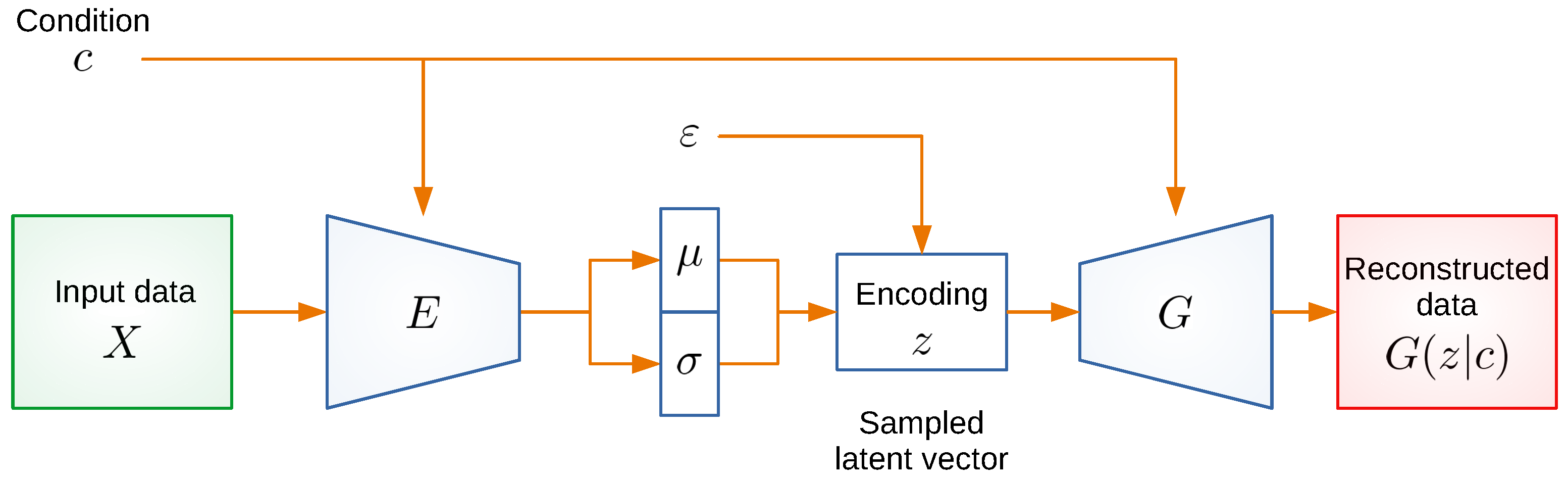
where ⊙ denotes the element-wise product. This transformation makes z appear as if it was drawn from N ( μ , σ ) while keeping the sampling operation differentiable. Thus, the reparameterization trick ensures that the gradients with respect to μ and σ can be calculated, making the training process using backpropagation feasible [53]. Analogous to cGANs, the VAE framework can be extended to a conditional VAE (cVAE), which incorporates additional input information c to guide the generative process. A schematic architecture of the cVAE is shown in Figure 3. The corresponding objective function of a cVAE is defined as
L c V A E ( E , G ) = E z E ( X , c ) | | X G ( z | c ) | | 2 2 + λ K L 1 2 ( 1 + log ( σ 2 ) μ 2 σ 2 )
where μ and σ depend not only on the input image X, but also on the conditional input c.

3. Materials and Methods

3.1. Experimental AC Dataset

The experimental data from AC are used for data synthesis and separation kinetic classification. Experiments are performed using the LUMiSizer instrument with disposable measurement cells (LUM GmbH, Berlin, Germany). In the simplest scenario, the sample comprises a continuous phase (liquid) and one disperse phase (particles or droplets). At the start of the measurement, the disperse phase is expected to be homogeneous and uniformly distributed, indicated by a constant extinction value over the length of the measurement cell. As a result of the centrifugal acceleration, the dispersed phase begins to settle or float, depending on the density difference between the liquid and the particles. Consequently, the light is obstructed depending on the local concentration, usually forming an extinction gradient. After the data are recorded, comprehensive analysis can be performed. However, the first step is to determine the main separation class in order to choose the proper algorithm for further analysis.
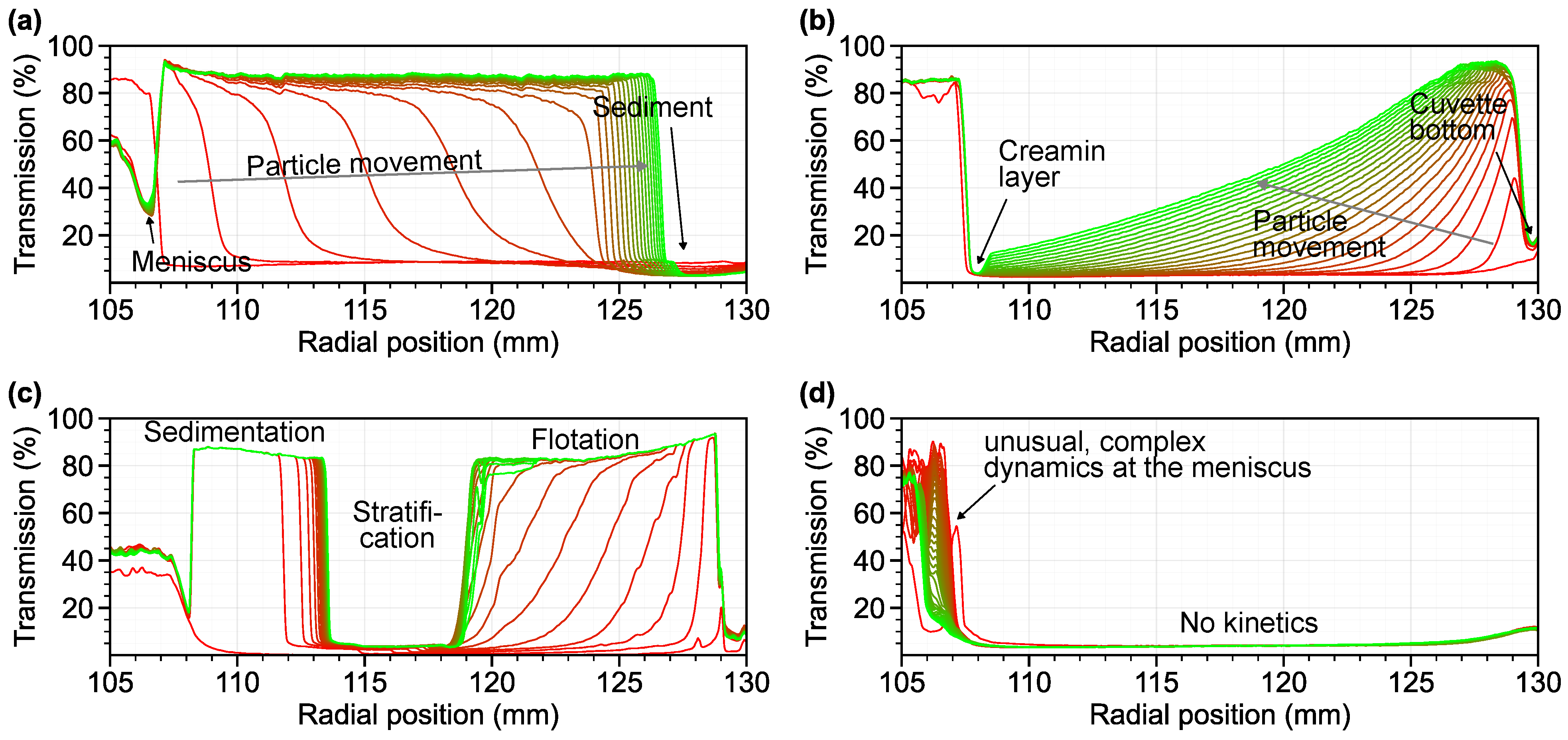
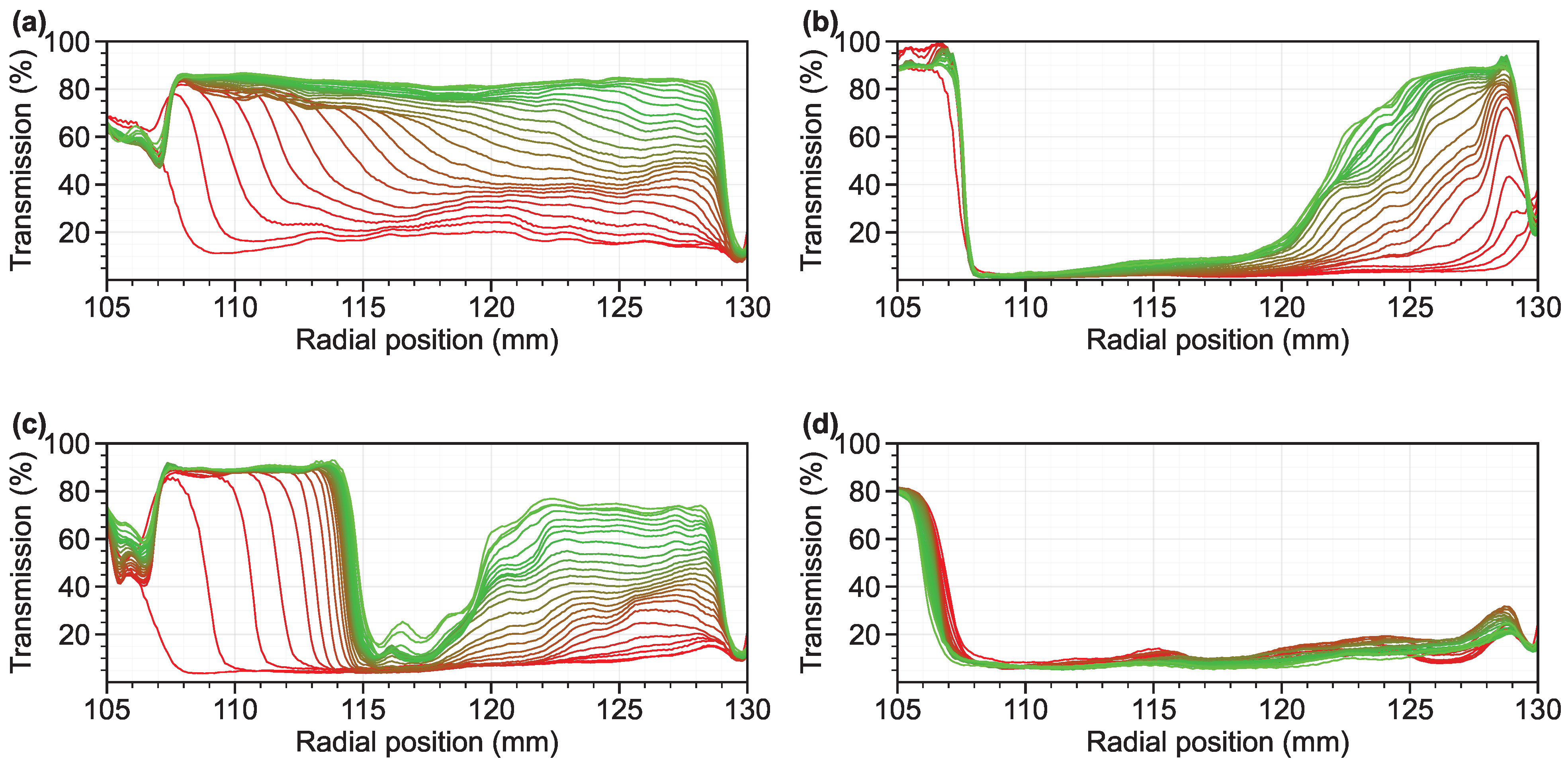
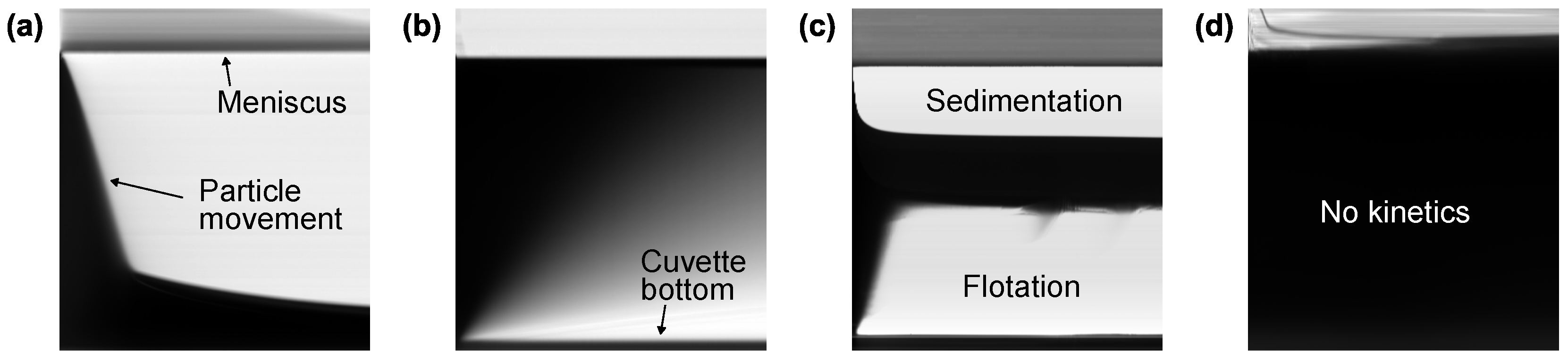
Figure 4 visualizes different representative samples for the four classes considered in this work. Transmission values are depicted over time (color-coded) and position (abscissa). The detection area spans approximately 25 mm (radial position from 105 mm to 130 mm). The bottom of the cell is located at 130 mm. The meniscus, located on the left side of the visualizations (usually between 106 and 108 mm), forms at the air-sample boundary due to the refraction of incident light. At each time step, a transmission profile is recorded covering the entire sample. For visualization purposes, the time vector is color-coded. As indicated, the first profile corresponds to the initial recorded measurement and is plotted with red color, and as time progresses, the color of the profiles shifts towards green. Consequently, the last recorded profile is visualized in green. By analyzing the patterns of the transmission profiles, one can classify different types of separation behavior. In this study, the observed phase separation behaviors were categorized into four distinct classes. These include sedimentation (SED, see Figure 4a), characterized by the settling of solid particles towards the bottom of the cell, flotation (FLT, see Figure 4b), involving the upward migration of particles or droplets; and sedimentation-flotation (SFL, see Figure 4c), where both settling and flotation mechanisms contribute to the overall separation dynamics. The theoretical difference of sedimentation and flotation is in the sign of the sedimentation velocity. However, the experimental data obtained do not exhibit a simple mirrored appearance. For instance, the meniscus does not look identical in the two cases. Additionally, floating particles and droplets in industrial and real-world systems are often broadly distributed, which results in sedimentation boundaries that are less sharp than those depicted in sedimentation classes. A fourth category, other (OTH), as seen in Figure 4d, was designated for cases exhibiting atypical or ambiguous behavior that does not conform clearly to the primary mechanisms and also includes failure measurements or highly stable dispersions with no kinetics.
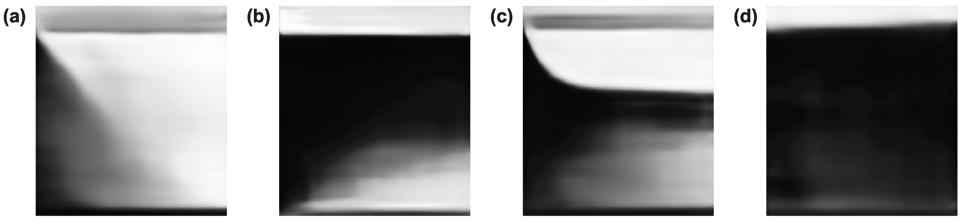
Within the first three classes, various subclasses exist, which are determined by the properties of the dispersed phase. These properties can include being monomodal, polymodal, monodisperse, and polydisperse. In addition, in the separation of complex products, various factors such as flocculation or aggregation, to name a few, can come into play and are included in the time dependent data. The dataset used in this study comprises 463 instances. To specify, the distribution of mechanisms within the defined classes is as follows: 269 instances of SED, 118 instances of FLT, 45 instances of a combination of SFL, and 31 instances categorized as OTH. Although the first two classes are predominant, it is important to note that the dataset exhibits an unbalanced class distribution. The data were randomly collected from a much larger measurement database compiled over decades and, on average, reflect the typical occurrence probabilities observed in real-world scenarios. While classification based on colored image representations can be intuitive, it may introduce unnecessary complexity due to the high-contrast color gradients, which are visually dominant. To mitigate this effect and maintain interpretability, an alternative grayscale visualization was employed [55]. Grayscale images (Figure 5) were generated from the corresponding transmission profiles by resizing the spatial and time resolution to 256 × 256 via interpolation. In this representation, transmission values from 0% to 100% are mapped to grayscale values between 0 and 256, with radial position (from top (meniscus) to bottom) on the ordinate, and time (from left to right) on the abscissa. This format preserves the essential spatial and temporal information related to particle migration during AC.

3.2. Simulated AUC Dataset

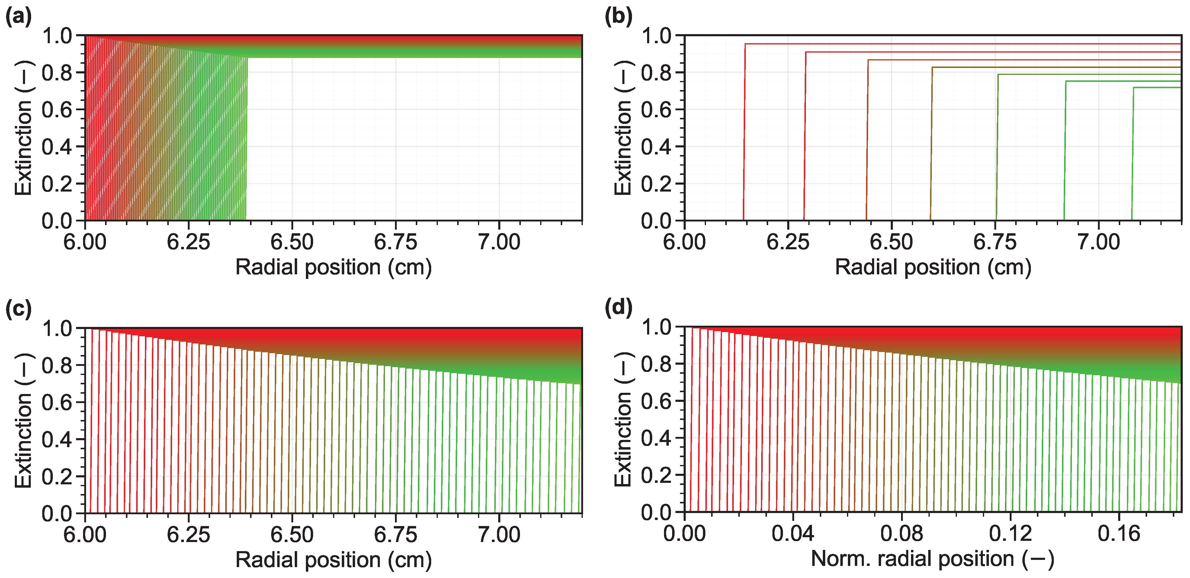
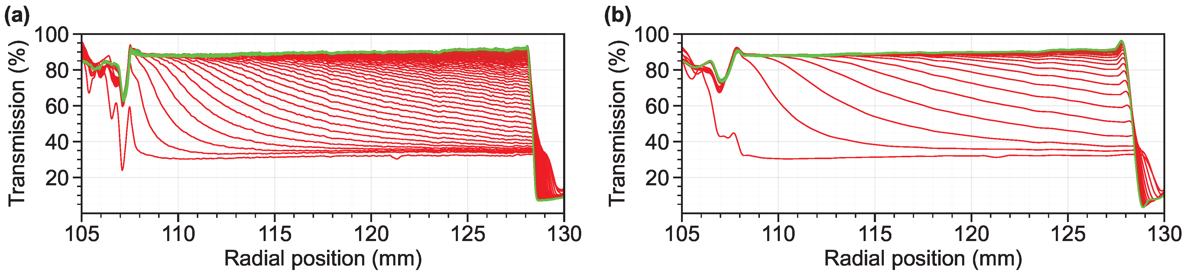
For the training of generative models and a regressor for sedimentation coefficient estimation, sedimentation experiments were simulated using a Direct Boundary Model (DBM) [37] approach in MATLAB (version R2021b). In each experiment, particles were simulated in sector-shaped cells, with the meniscus position at 6 cm and the bottom at 7.2 cm from the center of rotation. The measurement cell was divided into 280 equally sized bins, resulting in a radial resolution of around 43 µm. The synthetic datasets were generated for a fixed rotor speed of 2000 rotations per minute over a period of 2 h with a scan interval of 60 s, resulting in 120 scans per experiment. Without being restricted to a specific material system with a specific size and density, it was decided to generate datasets for different sedimentation coefficients without considering the effect of diffusion. Therefore, sedimentation of monodisperse systems with a sedimentation coefficient between 0 and 100,000 Sved was simulated in steps of 500 Sved, resulting in 201 datasets, based on the step function for sector-shaped cells. This range therefore covers material systems with a very low density, such as polymers (i.e., 1050 kg/m3 for polystyrene) between 10 nm and 1000 nm, as well as materials with a very high density, such as gold (19,320 kg/m3) between 10 nm and 100 nm. This reflects the typical areas of application for AUC in the field of particle measurement technology. Figure 6 shows the sedimentation profiles, which exhibit ideal behavior.
The visual appearance of the profiles changes with increasing sedimentation coefficient as the profiles are further apart, when the scan interval and rotor speed are kept constant. Additionally, at low sedimentation coefficients, the sedimentation process is incomplete as all particles have not yet reached the bottom of the cell after 2 h (Figure 6a). With large sedimentation coefficients, particle movement occurs quickly, resulting in only a few visible sedimentation profiles within the duration of the measurement (Figure 6b). With regard to a complete training data set, it is important to consider the variations of experimental parameters, such as rotor speed, time, and scan interval. It should be noted that different combinations of sedimentation coefficients and experimental parameters can lead to the formation of the same visual profile for a monodisperse sample, when diffusion is neglected. For instance, small particles in a high centrifugal field and large particles in a low centrifugal field can have the same sedimentation profile pattern. To eliminate any ambiguity in the data, a dimensionless sedimentation index is used:
θ ( s , t ) = s t 0 t 1 ω ( t ) 2 t d t
With this expression, each individual sedimentation profile can be described by a specific sedimentation index in its metadata, regardless of particle properties and experimental parameters. In this work’s training dataset, the sedimentation coefficient is a scalar value, representing a monodisperse particle species. As a result, θ only increases from left to right in the measurement profiles due to the integral term over ω ( t ) 2 t . The dimensionless radial position ln ( r / r m ) is introduced to account for varying radial positions in each experiment. Notably, this would allow for the inclusion of the training data from AC, too. Figure 6c,d demonstrate the normalization of the meniscus position to 0 using the dimensionless radial position. By the introduction of these dimensionless numbers, we can generalize the datasets for training of the DL model and reduce the number of parameters.

3.3. Proposed Approaches

3.3.1. Conditional VAE-GAN/VAE-WGAN

cVAEs model a structured latent space and promote diversity in generated samples, but they often produce blurry outputs. In contrast, cGANs generate sharp and realistic images through adversarial training, yet they lack a well-structured latent space. The proposed conditional Variational Autoencoder Generative Adversarial Network (cVAE-GAN) combines a cVAE and a cGAN, as illustrated in Figure 7, solving the limitations of each individual model. This architecture consists of three submodules: the encoder E, the decoder/generator G, and the discriminator D. The total objective of the proposed cVAE-GAN is defined as a weighted combination of two loss components:
L c V A E - G A N ( E , G , D ) = L c V A E ( E , G ) + λ a d v L c G A N ( E , G , D )
where λ a d v is a hyperparameter that controls the balance between reconstruction quality and adversarial regularization. The L c V A E term was introduced in Equation (22), while the L c G A N term, now also depending on E, is defined as follows:
L c G A N ( E , G , D ) = E ( X , c ) p d a t a ( X , c ) [ log D ( X | c ) ] + E z E ( X , c ) [ log ( 1 D ( G ( z | c ) | c ) ) ]
where G ( z | · ) represents the output of the generator given the latent variable z, and D ( · | c ) denotes the conditional discriminator. Similarly, a conditional Variational Autoencoder Wasserstein Generative Adversarial Network (cVAE-WGAN) can be constructed by combining the cVAE loss L c V A E with a cWGAN loss L c W G A N , defined as
L c W G A N ( E , G , C ) = E ( X , c ) p d a t a ( X , c ) [ C ( X | c ) ] E z E ( X , c ) [ C ( G ( z | c ) | c ) ]
where G ( z | · ) represents the reconstruction from the cVAE given the input image X, and C ( · | c ) denotes the conditional critic.

3.3.2. Physical Constraint of AUC Data Synthesis

The AUC dataset described in Section 3.2 contains sedimentation experiments simulated under ideal conditions, where particles always travel toward the bottom of the cell. To incorporate this behavior into generative models, a Physical Constraint (PhysC) is introduced as an additional loss term, defined as
L P h y s C ( G ) = i , j ReLU i G ( z | c ) + ReLU j G ( z | c )
where i G ( z | c ) and j G ( z | c ) represent the gradients of the generated data G ( z | c ) along its spatial directions:
i G ( z | c ) = G ( z | c ) i , j G ( z | c ) i 1 , j j G ( z | c ) = G ( z | c ) i , j G ( z | c ) i , j 1
with i and j denoting the indices for the columns and rows within the grayscale image, respectively corresponding to the vertical and horizontal spatial dimensions. By applying Rectified Linear Unit (ReLU) to the spatial gradients, we penalize positive changes in intensity, ensuring that the produced synthetic data remains largely homogeneous and allowing for, at most, a single sharp transition that represents a sedimentation front.

3.3.3. Generative Models with Physical Constraint

By incorporating PhysC, we introduce cWGAN with PhysC (cWGAN-PhysC) and cVAE-GAN with PhysC (cVAE-GAN-PhysC) approaches. The corresponding objectives are defined as follows:
L c W G A N - P h y s C ( G , C ) = L c W G A N ( G , C ) + λ P h y s C L P h y s C ( G )
L c V A E - G A N - P h y s C ( E , G , D ) = L c V A E - G A N ( E , G , D ) + λ P h y s C L P h y s C ( E , G )
In both equations, λ P h y s C denotes a weighting factor that controls the contribution of the physical constraint loss term to the overall total objective.

3.4. Implementation Details

3.4.1. Conditional GAN/WGAN

The generator receives a random noise vector of size 256, which is concatenated with the conditional scalar input, which can be either a class ID (used in the AC dataset) or a sedimentation coefficient (used in the AUC dataset). It comprises a sequence of transposed convolutional layers with 2 × 2 kernels, followed by two additional convolutional layers. Each layer is equipped with batch normalization and ReLU activation. The number of kernels starts at 1024 and is halved at each successive upsampling stage. The final layers return single-channel synthetic data. Both the generated data and the original input data are fed into the discriminator/critic, along with the corresponding conditional input. To incorporate this input, a conditional image is produced and concatenated with the input image along the channel dimension. If the conditional input is a class ID, it is first transformed into a one-hot encoded vector, which is then passed through an embedding layer. The resulting embedded vector is tiled spatially to match the dimensions of the input image, forming the conditional image. In the case of a sedimentation coefficient, the scalar value is directly repeated across the spatial dimensions to produce a conditional image of the same size as the input image. The discriminator/critic consists of six resolution levels, each employing strided convolutions with 4 × 4 kernels and a stride of 2 in both spatial dimensions. Each convolution is followed by batch normalization and a leaky ReLU activation with a negative slope of 0.2. The number of filters starts at 32 and doubles at each subsequent resolution level. The final activation depends on the type of the network: a sigmoid is applied in the discriminator, while no activation is used in the critic.

3.4.2. Conditional VAE

The encoder of the cVAE takes two inputs: an image and a conditional input (class ID or sedimentation coefficient). Initially, the conditional input is a scalar, and it is incorporated into the network in the same manner as in the discriminator/critic of cGAN/cWGAN. The encoder consists of six resolution levels (excluding the bottleneck), with two convolutional layers at each level. Each convolution uses 3 × 3 kernels, followed by batch normalization and a ReLU activation. The number of filters starts at 32 and doubles at each successive resolution level. Max pooling is applied for subsampling. At the bottleneck resolution, the extracted features are transformed into a bottleneck vector of size 4096 employing a single convolutional layer. This vector is then split into two vectors of size 2048, representing the learned mean ( μ ) and standard deviation ( σ ). A reparameterization (see Section 2.5) is applied to these vectors, producing the sampled latent vector of size 2048. This vector is then concatenated with the conditional prior before being passed to the decoder/generator. The VAE decoder employs a sequence of transposed convolutions using 2 × 2 kernels, followed by two additional convolutional layers. A 1 × 1 convolution is used as the last layer, with a hyperbolic tangent function applied as the final activation.

3.5. Training Details

3.5.1. Training with AC Dataset

All models were implemented in Python (version 3.10.8) using the PyTorch framework [56] (version 1.13.1) and trained on NVIDIA RTX A6000 GPUs with 48 GB VRAM. The computational experiments were containerized using Docker (version 24.0.3). Modeling with the AC dataset were conducted using five-fold cross-validation, with a 60%-20%-20% split for training, validation, and testing, respectively. To address the class imbalance across the four classes, stratified splitting was performed to preserve class proportions in each subset [57]. Since the original sequences vary in both spatial and temporal resolution, all grayscale images (see Figure 5) were uniformly resized to a fixed resolution of 256 × 256 pixels by interpolation to ensure consistent input dimensions for subsequent processing and model training. Additionally, the resized dataset, containing transmission values in percentage, was normalized to the range [−1, 1]. The cVAE-WGAN model was trained for a total of 2100 epochs using the RMSProp optimizer [58], with a learning rate of 0.0002 for both the encoder and decoder/generator, and 0.0004 for the critic. Training began with a 100-epoch warm-up phase, during which the cVAE was pretrained using only the reconstruction loss. This was followed by 2000 epochs of joint training, incorporating the adversarial objective and a KL divergence term weighted by λ K L = 50 .

3.5.2. Training with AUC Dataset

All experiments using the AUC datasets were evaluated using leave-one-out cross-validation. The datasets were split into training, validation, and testing sets in a 60%-20%-20% ratio. The split followed a systematic approach: the data was first divided into sequential bins of five samples, and each bin was then partitioned according to the specified ratio. This ensured that each subset captured a representative range of sedimentation coefficients. The input data, which corresponds to the grayscale image representation, was resized to a spatial resolution of 256 × 256 pixels by interpolation and normalized extinction data to the range [−1, 1] prior to training. The cWGAN model was trained for 10,000 epochs. As noted in [52], training WGANs with momentum-based optimizers such as Adam can lead to instabilities [59]. Therefore, RMSProp was used instead [58]. During critic training, a gradient penalty term was included following the approach in [60]. Additionally, the training adhered to the Two Time-Scale Update Rule [61], using learning rates of 0.0002 for the generator and 0.0004 for the critic. The training was conducted with mini-batches of 32 samples. The cVAE model was trained for 1000 epochs using the Adam optimizer [59] with parameters β 1 = 0.9 and β 2 = 0.999 , and a learning rate of 0.01. The KL divergence weight λ K L was set to 1. A mini-batch size of 16 was used during training. The cVAE-GAN model was trained for 2500 epochs using the Adam optimizer [59], with learning rates of 0.0002 and 0.0004 for the generator and discriminator, respectively. One-sided label smoothing was applied during adversarial training, where soft target values (e.g., 0.9 for real and 0.1 for fake) were used instead of hard binary labels, following the approach in [62]. The KL divergence weight λ K L was set to 20. A mini-batch size of 16 was used. The cWGAN-PhysC and cVAE-GAN-PhysC models, which incorporate PhysC, used the same architectures and training configurations as their unconstrained counterparts. For cWGAN-PhysC, the PhysC weight λ P h y s C was set to 1. For cVAE-GAN-PhysC, λ P h y s C was set to 5.

4. Evaluation Methods and Metrics

4.1. Qualitative Analysis

4.1.1. Visual Comparison of Principal Components

Principal Component Analysis (PCA) was used to project sedimentation boundary data onto a new coordinate system defined by uncorrelated components, called principal components (PCs), which are aligned with the directions of greatest variance [63]. The leading components capture the most prominent patterns, enabling clearer visualization and aiding the classification of separation kinetic classes. PCA was performed on both real and synthetic AC data using the Python implementation via scikit-learn [64]. For interpretability and visualization purposes, the analysis focused on the first three PCs, which are then compared and discussed.

4.1.2. Visual Comparison in Image Space

To assess the realism of the synthesized data, a representative subset of 10–11 examples per class was selected, resulting in 43 instances each for the experimental and synthetic datasets. For perceptual evaluation, a randomized slideshow of the color-coded images (86 total instances, including experimental and synthetic data) was presented to participants with varying levels of domain expertise. A two-part expert assessment was conducted involving three categories of participants with different levels of AC expertise, a Beginner Knowledge Category (BKC, n = 3), an Intermediate Knowledge Category (IKC, n = 3), and an Advanced Knowledge Category (AKC, n = 1). The BKC consisted of individuals who had received AC training, conducted experiments, and performed basic data analysis. The IKC included interdisciplinary researchers who regularly analyze AC data, but whose primary focus lies in other scientific fields. The AKC comprised a single expert with several years of experience in AC. Without prior information on their origin, participants were asked to label each image as either real or synthetic. After that, the participants were shown randomly ordered experimental data representing the four predefined classes: SED, FLT, SFL and OTH. Based solely on visual inspection, they were required to assign each image to one of the four classes. The resulting accuracy metrics from both tasks serve as a baseline for comparison with automated classification models.

4.2. Quantitative Analysis

In the domain of generative models, the Fréchet Inception Distance (FID) is a commonly used metric for assessing the similarity between distributions of real and synthetic images [61]. Originally proposed as an improvement over the Inception Score, FID measures the Fréchet (Wasserstein-2) distance between multivariate Gaussian distributions fitted to the feature representations of real and synthesized images. These features are typically extracted using a pretrained convolutional neural network. Formally, if the real features follow a normal distribution with mean and covariance ( μ r e a l , Σ r e a l ) , and the synthetic features follow ( μ s y n t , Σ s y n t ) , then the FID is defined as
FID = | | μ r e a l μ s y n t | | 2 2 + Tr ( Σ r e a l + Σ s y n t 2 Σ r e a l Σ s y n t )
where Tr denotes the trace of a matrix. The metric captures both, the difference in means and the discrepancy in the covariance between real and synthesized features. A lower FID value indicates high similarity and a higher FID value indicate differences in the datasets.
One important metric is accuracy and is defined as the ratio of correctly predicted samples to the total number of predictions:
Accuracy = ( TP + TN ) / ( TP + TN + FP + FN )
Although accuracy is a straightforward performance measure, it can be misleading in cases of imbalanced datasets where one class dominates the others. To better understand a model performance in such contexts, precision and recall are often considered. Precision quantifies the proportion of correctly predicted positive samples among all predicted positive samples:
Precision = TP / ( TP + FP )
On the other hand, recall measures the proportion of correctly identified positive samples among all actual positives and is crucial when the consequences of missing positive instances are severe. It is computed as
Recall = TP / ( TP + FN )
Balancing precision and recall is achieved through the F1 score, which is the harmonic mean of the two metrics. The F1 score is given by
F 1 = 2 · ( Precision · Recall ) / ( Precision + Recall )
thus favoring models that perform well on both dimensions, especially in imbalanced classification tasks. For regression tasks, several metrics are used to assess the accuracy of continuous predictions. One of the most common is the MSE. It is calculated as the average of the squared differences between predicted and actual values:
MSE = 1 n i = 1 n ( y i y ^ i ) 2
where y i is the true value, y ^ i is the predicted value and n the total number of instances. This metric penalizes larger errors more heavily, making it sensitive to outliers. To make the metric more interpretable in the original units of the target variable, the Root Mean Squared Error (RMSE) is used:
RMSE = 1 n i = 1 n ( y i y ^ i ) 2
RMSE retains the same penalization of large errors but allows for easier interpretation in practice. Another widely used metric is the Mean Absolute Error (MAE), which averages the absolute differences between predicted values and actual values. It is given by
MAE = 1 n i = 1 n | y i y ^ i |
Unlike MSE, MAE treats all errors linearly and is therefore less sensitive to large deviations. In addition, the coefficient of determination R2, quantifies the proportion of variance in the dependent variable that is explained by the model. It is computed as
R 2 = 1 [ ( y i y ^ i ) 2 / ( y i y ¯ ) 2 ]
where y ¯ is the mean of all observed values y ^ i . The value of R2 ranges from negative infinity to one, with a value of one indicating perfect prediction.

5. Results and Discussion

5.1. Synthetic AC Data

AC data were synthesized using the cVAE-WGAN architecture. The synthesized data were subsequently compared with experimental measurements, through human evaluation, and quantitatively using the FID score. Figure 8 illustrates representative examples of synthesized profiles for each of the predefined classes. At a glance, the essential physical features appear consistent across all cases and are comparable with the visualization of the real experiments in Figure 4. The features of the sedimentation and flotation processes (moving sedimentation boundaries) are clearly observable. In Figure 8a, the sedimentation boundary is seen to progress from the meniscus towards the bottom of the cell, which is a characteristic feature of a sedimentation process. In contrast, Figure 8b shows flotation behavior, where the sedimentation boundary moves from the bottom of the cell to the meniscus. In the combined case (Figure 8c), both behaviors are present, a boundary moves downwards from the meniscus, while simultaneously a broader boundary forms at the bottom and ascends. This results in a concentrated central region (stratification), consistent with the pattern observed in Figure 4c. Figure 8d shows almost no transmission kinetic, in line with expectations based on experiments, as shown in Figure 4d. Upon closer inspection, in Figure 8a, the initial transmission values (10–20%) show uncommon fluctuations over the complete sample height. In a well-homogenized sample, these initial transmission values are expected to remain uniform across the sample region. In Figure 8b, the sedimentation boundaries show unusual local fluctuations, whereas in Figure 4b, the boundaries appear smooth and uniform. Figure 8c exhibits atypical high transmission values in the central region (115–120 mm), where high concentrations would typically yield lower and more constant transmission. Finally, in Figure 8d, an atypical color gradient is observed at the meniscus, where the boundary at radial position of approximately 107 mm shifts to a lower positions. This may indicate an apparent expansion of the liquid volume, which generally does not occur. Figure 9 presents the grayscale representations of the synthesized data shown in Figure 8. When comparing these synthesized class images with their experimental counterparts in Figure 5, it is evident that the transitions from low to high transmission (grayscale) values are significantly smoother and more gradual in the synthesized images. It should be noted that the colored sedimentation profiles shown in Figure 4 and Figure 8 represent only a selected subset of the available profiles, chosen to facilitate clearer visualization and interpretation. In contrast, the grayscale images in Figure 5 and Figure 9 are constructed using the complete set of profiles. The synthesized data contain 256 profiles, whereas the experimental data may include up to approximately 600 profiles. Consequently, the grayscale visualization of the experimental data can appear sharper due to the denser sampling of profiles used in constructing the image.
However, all of these interpretations require a certain level of expert knowledge. A notable feature shared by all synthetic datasets is their overall smoother appearance compared to experimental data. Experimental measurements are inherently influenced by electronic noise, which introduces small-intensity fluctuations across the entire measurement range. In contrast, these fluctuations are absent in the synthetic images, resulting in smoother profiles at the microscopic scale but a more smeared appearance in the macroscopic view, in particular in the colored data representations. This difference alone may allow one to distinguish between real and synthetic images without any specialized physical understanding. To mitigate this bias prior to human classification, the experimental data are pre-processed to resemble the synthetic results more closely, while preserving the underlying physics. To ensure the desired comparable visual appearance, the experimental data undergo additional smoothing using a Savitzky–Golay filter [65] as implemented in the SciPy library [66]. Additionally, the synthetic data have a constant number of transmission profiles (time stamps), whereas the experimental data range from 60 to 600 profiles, in dependence of the original measurement set-up. Therefore, a pre-processing step is applied to reduce the number of profiles in the experimental data to approximately 100 profiles. The impact of data pre-processing on transmission profiles is illustrated in Figure 10. Figure 10a displays the unprocessed data from a sedimentation experiment, and Figure 10b shows the corresponding representation after applying profile reduction and smoothing. This step makes the visual appearance of the experimental data more similar to that of the synthetic data, without altering the kinetic separation behavior. Turning to the classification accuracy across the expert groups, BKC achieved an average accuracy of (63.1 ± 6.4)%. This is only slightly better than chance. IKC performed substantially better, with an average accuracy of (81.3 ± 5.1)%. AKC reached an accuracy of 97.7%, suggesting that even experienced individuals may occasionally be misled. For the purpose of this paper, the cVAE-WGAN successfully produced synthetic sedimentation profiles that closely mimic experimental transmission data. For individuals without prior expertise in the analysis of sedimentation boundaries, distinguishing between experimental and synthetic profiles is difficult.
For comparison to the human-based evaluation, the FID is calculated to assess the similarity between real and synthetic data. For FID calculation, the original feature representation of the cVAE-WGAN network is used without the pre-processing step for human assessment. The resulting FID score is 143, indicating a notable distributional gap between experimental and synthesized instances. In the field of generative modeling of natural images, particularly using high-resolution facial datasets, FID scores below 5 have been achieved [67]. In contrast, for industrial surface defect classification tasks, reported FID scores are typically around 130, which is considered an acceptable threshold for reliable classification performance [68]. While the literature suggests that there is potential to further improve the data generator employed in this study, such enhancements are beyond the scope of the present work.

5.2. Principal Component Analysis of AC Data

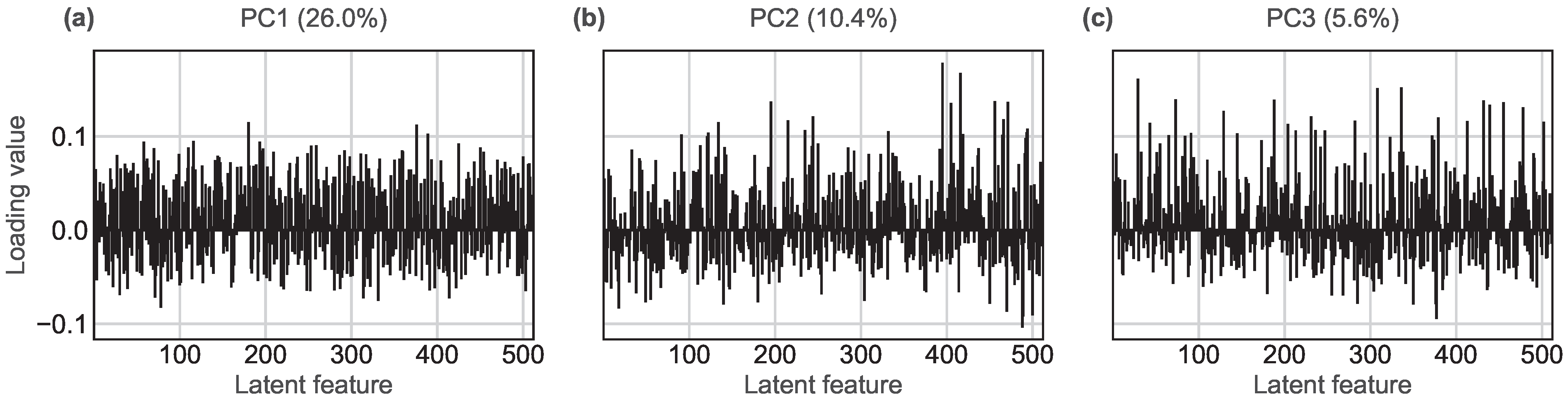
PCA was performed on the 512-dimensional feature vectors extracted from the penultimate global average pooling layer of the trained ResNet34 classification model using AC data (e.g., Figure 4). ResNet34 was chosen for its widespread applications in image classification tasks. These latent vectors encode high-level representations of the transmission scan images (radial position versus time). Thus, PCA was not applied directly to the resized 256 × 256 grayscale images, but rather to their deep feature embeddings. Consequently, the principal component loadings represent linear combinations of learned ResNet34 features rather than physically interpretable variables. The first three PCs explain 26% (PC1), 10.4% (PC2), and 5.6% (PC3) of the total variance, respectively. The loading distributions of PC1 to PC3 across all 512 latent features are shown in Figure 11a–c. PC1, which captures the largest proportion of variance (26%), exhibits loading values within the range of 0.08 to + 0.11 . These loadings are broadly and evenly distributed across the 512 latent features, with many features contributing with moderate magnitude and alternating signs. PC2 (10.4% variance) displays a more heterogeneous loading profile. Unlike PC1, the contributions are less uniformly distributed, instead showing more isolated positive and negative peaks concentrated in specific feature regions. PC3 accounts for 5.6% of the total variance and exhibits an even more heterogeneous and irregular loading distribution than the former two. Overall, the loading distributions suggest a hierarchical organization of variance in the latent space.
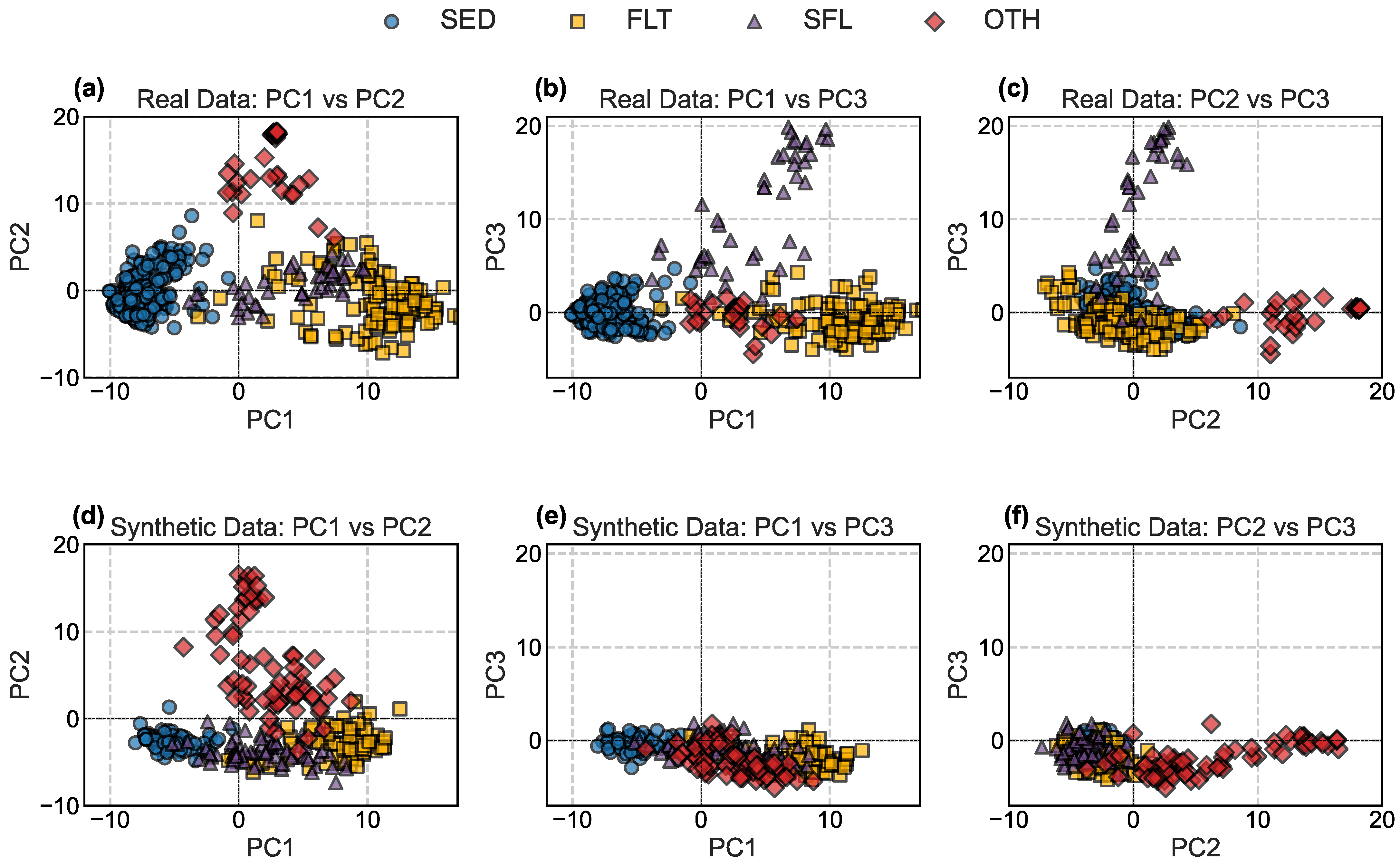
In Figure 12, the first three principal components (PC1–PC3) of the ResNet34 latent feature space are shown as pairwise two-dimensional projections for the real dataset (a–c) and the synthetic dataset (d–f). Instances of SED (blue circles) are tightly clustered with relatively low variance and a consistent tendency toward negative PC1 values. Among the classes, SED is visually the most well-separated from the others. In contrast, FLT (yellow squares) tends to lie on the opposite side of PC1, displaying predominantly positive PC1 values. However, FLT is more dispersed compared to SED, particularly in PC1, which could make them more challenging to classify. Nevertheless, the spatial distribution of FLT is broadly consistent between the real and synthetic datasets. SFL (purple triangles) exhibits a distinct pattern in the real dataset, with many samples showing high positive PC3 values (see Figure 12b,c). This separation is not observed in the synthetic dataset (Figure 12e,f), where the distribution of this class is centered closer to zero across all components. Additionally, the variance within SFL is noticeably higher in the real data compared to the synthetic. OTH (red diamonds) is primarily associated with higher PC2 values in both datasets. However, in the real data, the samples are more tightly clustered at higher PC2 values, while in the synthetic dataset, they are more broadly distributed and extend towards zero. Apart from this difference in spread, the overall positioning of the class is relatively similar in both datasets. In summary, PC1 appears to provide a strong axis of separation between SED and FLT, with minimal overlap between them. SFL and OTH intersect more noticeably with the former two classes in PC1, reducing their separability. PC2 is dominated by features of OTH, although some overlap with FLT exists. In the synthetic dataset, SFL overlaps considerably with both SED and FLT, which makes classification more complicated. However, in the real dataset, its pronounced extension along PC3 may aid in distinguishing it from the other classes. These PCA observations suggest that, even without dimensionality reduction, human classifiers are likely to distinguish SED and FLT relatively reliably. SED, in particular, forms a dense cluster, which may allow humans to classify it with the highest accuracy. In contrast, SFL overlaps considerably with FLT, making these two classes the most challenging to distinguish. The OTH class may be somewhat easier to identify, owing to its relatively good separation along PC1.

5.3. Classification of Separation Kinetics

Finally, neural networks were used to classify different separation kinetics. The evaluation included two widely used architectures, ResNet34 (trained on color images, COL, and grayscale images, GRY) and a Transformer, as well as two standard recurrent neural networks: Long Short-Term Memory (LSTM) and Gated Recurrent Unit (GRU).
The color images (COL) represent the temporal evolution of transmission, with each scan corresponding to one time point and the progression of time encoded in a color gradient from red to green. The grayscale images (GRY) provide an alternative visualization of the same data, scaled to 256 × 256 pixels, where the vertical axis represents radial position and the horizontal axis represents time. Transmission values are mapped to 8-bit grayscale (0 = black, 255 = white), where white indicates 100% transmission and black 0% transmission. ResNet34-COL refers to the model which is trained on the visual presentation of the transmission scans where the time evolution is color-coded (e.g., Figure 8), whereas ResNet34-GRY is the model trained on the resized and normalized grayscale representation (e.g., Figure 9).
The first section of the Table 1 presents the class-sensitive accuracy metrics of the used models trained on experimental data, providing the classification accuracy for each individual class. All models perform quite well, particularly for SED. ResNet34-GRY, together with Transformer and LSTM, achieved the highest accuracies of around 99.3%. The lowest-performing model, GRU, reached 97%, which is still a strong performance. For FLT, accuracy is more variable, ranging from approximately 79.7% for LSTM to 91.5% for ResNet34-COL, but the overall performance is still reasonably good. This trend aligns with the data distribution in the experimental dataset, where SED and FLT were the most represented classes and also with the distinguishable distributions of the PCs in Figure 12. For the remaining two classes, SFL and OTH, most models perform poorly. Notably, ResNet34-COL achieves moderate accuracy for these underrepresented classes, followed by ResNet-GRY. Both outperforms the RNN-based models. ResNet34-COL, trained on colored transmission data images (see Figure 4), delivers the highest class-sensitive accuracy. This may be attributed to the rich feature representation in the colorful plots. However, this approach heavily depends on fixed visual formats, including axes, ticks, and labels, making it less adaptable to changes in visualization style. In addition, it does not explicitly consider the sequential nature of the data. In contrast, sequential models like LSTM and GRU, which process raw time and position data, are inherently better suited to capture temporal dependencies. The LSTM performs comparably to the ResNet34 architectures for SED (around 99%) but underperformed for the other classes. The GRU, on the other hand, shows slightly lower accuracy for SED but exceeds LSTM in the remaining three classes. The Transformer model, used as a potential alternative, offers results slightly below ResNet34, but better than both RNN-based architectures overall.
To improve model performance, particularly for the underrepresented classes, synthetic images were synthesized and manually curated by the authors. This process resulted in a balanced dataset comprising 400 synthetic instances (see Figure 8), 100 per class, which were subsequently used to fine-tune (FTN) all models. The class-specific accuracy results are presented in the second section of Table 1. The impact of the additional training step on class-sensitive predictions is mixed, but overall it generally improves model performance. ResNet34-COL increased OTH prediction accuracy by around 13%, while the accuracies for SED and SFL showed slight decreases. In contrast, ResNet34-GRY lost significant accuracy for all classes except SED. The most notable improvements were observed for SFL and OTH in the sequential models, LSTM gained approximately 9% for FLT, 16% for SFL, and 42% for OTH, while GRU gained 1% for SED, 3% for FLT, 11% for SFL, and 45% for OTH. Transformer also showed gains in accuracy, though these were smaller than those of the sequential models. Despite the strong improvements from fine-tuning in the sequential models, ResNet34-COL remains the best overall model in terms of class-sensitive accuracy. For further comparison, a classification task with 83 instances was conducted by human participants with varying levels of domain expertise. The results are presented in the final section of Table 1. All human categories achieved their highest accuracy in classifying SED. Here, the expert (AKC) correctly classified all instances, while even the inexperienced users (BKC) achieved an accuracy of around 82%. This aligns with the PCA results and the dense clustering of the group SED inside the first 3 PCs. Interestingly, for FLT, both BKC and IKC performed markedly worse than the DL models, BKC reached only around 22% mean accuracy, while IKC achieved 63%. Even the expert misclassified a notable number of instances, resulting in an accuracy of 75%. For the underrepresented classes SFL and OTH, BKC performed poorly, with accuracies of 53% and 55%, respectively. IKC performed better, achieving 80% and 62% accuracies. However, all human categories were outperformed by the expert, who reached 90% and 100% accuracy for SFL and OTH, respectively.
The overall classification performance of the evaluated models and human participant categories is summarized in Table 2. The first section of the table presents the results for models trained on experimental data. Among these, ResNet34-COL emerged as the top-performing model across all reported metrics with accuracy, precision, recall and F1-Score greater than 93%, closely followed by ResNet34-GRY. Fine-tuning with synthetic data resulted in performance improvements across all models, as shown in the second section of Table 2. ResNet34-COL exhibited a modest gain in mean accuracy of 0.5%. Although this was the smallest relative improvement, ResNet34-COL remained the overall best performing model. The Transformer improved by accuracy by approximately 3%, while both the LSTM and GRU models showed substantial increases of around 6%. In general, all metrics are improved for LSTM, GRU and Transformer architecture. In the final section of Table 2, performance metrics for human participants are reported. BKC achieved an average accuracy of approximately 53%. IKC performed better, with an average accuracy of around 76%, while AKC reached 91%. Notably, the fine-tuned ResNet34-COL (94% accuracy) and most of the other models, not only outperformed both BKC and IKC, but also slightly exceeded the performance of AKC. The same discussion applies to the other metrics. These results underscore the potential of DL models to match and in some cases surpass human expert performance.

5.4. Synthetic AUC Data

The quality of synthesized AUC data is evaluated using neural network architectures and least-square direct boundary model [37]. In the former case, regression models are trained on a subset of the dataset described in Section 3.2 to learn the relationship between sedimentation boundary propagation and sedimentation coefficients for strictly monodisperse systems. The same models are used as for the AC dataset, with the ResNet34, which, due to its special architecture and residual blocks, is ideally suited for predictive tasks, as has already been shown in previous work [69]. Table 3 shows the training results, with ResNet34 achieving the best result (R2 = 0.998) and LSTM the worst (R2 = 0.882). The MSE, RMSE and MAE values demonstrate a similar pattern, with ResNet34 performing consistently better than the other models, followed by Transformer and GRU, and finally LSTM. As expected, the MSE is greater than the MAE because MSE is a quadratic measure. The RMSE is more comparable to the MAE. ResNet34 was also trained once with color images (COL) and once with grayscale images (GRY). In this case, both variants performed similarly well, with ResNet34-GRY showing slightly higher values: an MSE of 1,439,340 Sved2, an RMSE of 1200 Sved, and an MAE of 987 Sved.
For the synthesis of AUC data, different generative models, cWGAN, cVAE, a combination of cGAN and cVAE and with additional PhysCs, are tested. The quality and authenticity of the resulting sedimentation profiles are first evaluated using the trained ResNet34-GRY model, which achieved the best performance of all the different regression models, and the results are summarized in Table 4. Regarding the R2 measure, the synthetic data from cVAE-PhysC achieves the best result with a value of 0.996, while cVAE-GAN-PhysC achieves the worst result with a value of 0.983. In terms of MAE, the cVAE-PhysC also gives the best results with a value of 1339 Sved, while the cVAE-GAN-PhysC shows the poorest results with a value of 2939 Sved. The cVAE and cVAE-GAN network’s performances are intermediate between the cVAE-PhysC and cVAE-GAN-PhysC models. cWGAN with and without PhysC also reach a very high R2 value of 0.990, close to the performance of cVAE-GAN. The MSE and RMSE measures indicate the same ranking, with the MSE showing much larger values and the RMSE values being comparable to the MAE. Examining the FID measure now, the order of performance slightly changes. The cVAE-PhysC achieves a very good result of 150, indicating high data accordance in feature space, while the cVAE-GAN-PhysC model shows the worst performance with 912. The second-best model is the cWGAN with 220, followed by the cVAE-GAN with 280, cWGAN-PhysC with 422 and cVAE with 540. The very different results of the FID measure and the other metrics make interpreting the results difficult, as it is hard to tell which measure to rely on. Therefore, an additional evaluation of the model’s performance is necessary.
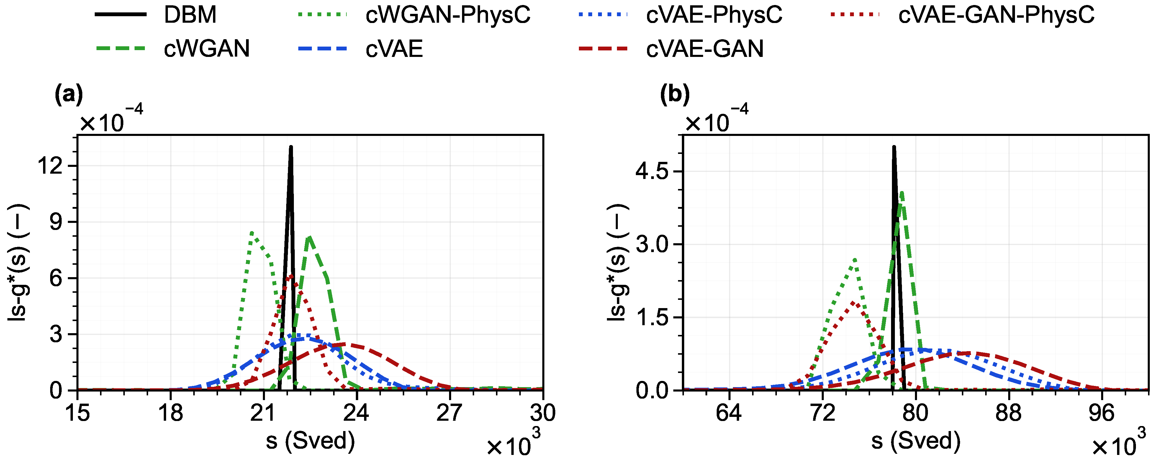
To further evaluate the synthesized data and compare the different generative models, the sedimentation profiles are analyzed using one of the standard methods for AUC, namely the ls-g*(s) model implemented in SEDFIT (version 16.1 c) [37], and the respective sedimentation coefficient distributions are determined. Since the models were trained using monodisperse systems, it was expected that the results would show no considerable distributions. However, the synthesized data contain additional noise from the networks, resulting in smeared sedimentation profiles and a distribution when the data are analyzed. The data are evaluated by comparing the calculated weight-average sedimentation coefficient value with the expected value, in order to describe the authenticity of the synthesized profiles. Figure 13 shows the sedimentation coefficient distributions obtained for the different generative networks, with expected values of 21,875 Sved (Figure 13a) and 78,125 Sved (Figure 13b). For comparison, these examples also contain the result of a DBM simulation analyzed using the ls-g*(s) model, which reflects the monodispersity of the particles as a narrow peak. On the one hand, the cVAE, cVAE-PhysC and cVAE-GAN model results show a significantly broader distribution, indicating a polydisperse system. On the other hand, combining cVAE-GAN with PhysC leads to a narrower distribution and achieves a good mean value for the 21,875 Sved example. The two models, cWGAN and cWGAN-PhysC, produce similar results, with the variant without PhysC providing slightly narrower distributions and a good mean value for the example of 78,125 Sved.
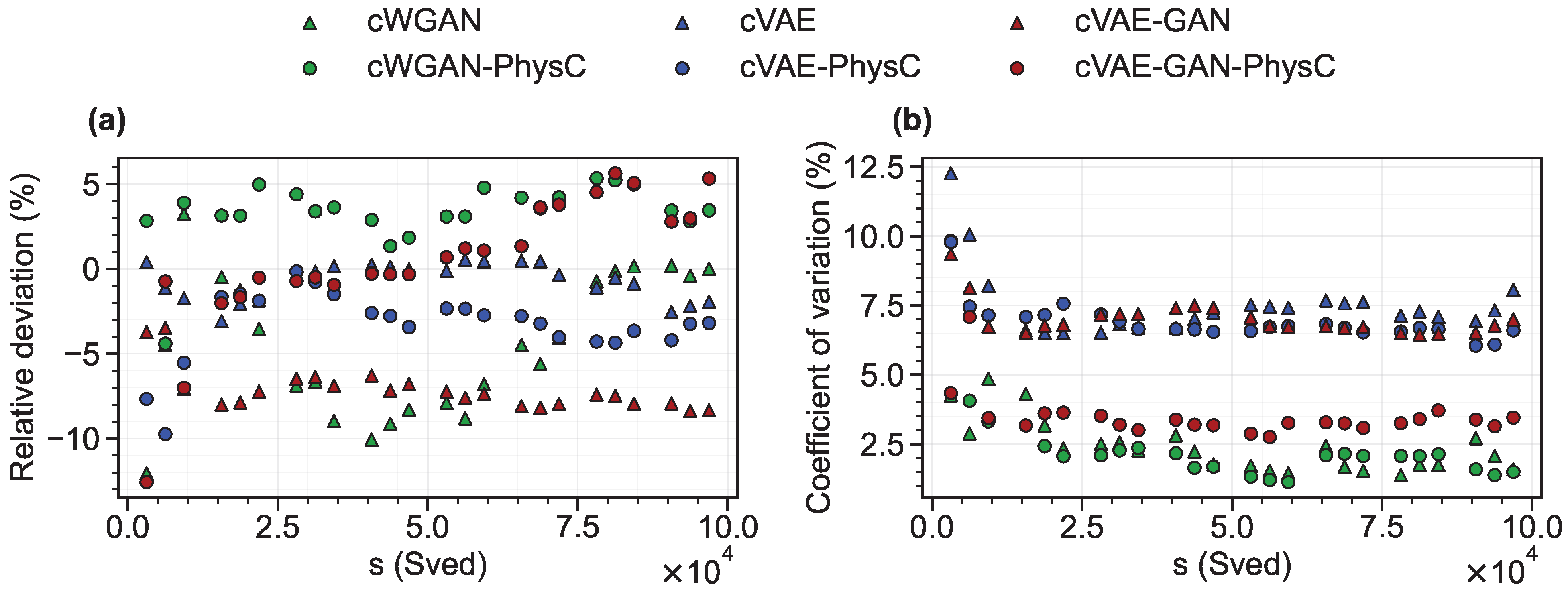
The results in Figure 13 indicate that the generative models cannot represent a wide range of sedimentation coefficients equally well (see cWGAN and cVAE-GAN-PhysC, for example). In order to assess the generalizability of the different models, 24 synthesized datasets are evaluated using the ls-g*(s) model. Figure 14a shows the relative deviation of the weight-average from the expected value, and Figure 14b depicts the coefficient of variation, which relates the standard deviation to the mean, as a measure of the width of the distribution for the six models. The relative deviation fluctuates considerably for cWGAN, but less so for cWGAN-PhysC. cVAE, cVAE-PhysC and cVAE-GAN also demonstrate minimal variation, with the latter exhibiting a systematic shift toward negative values. The cVAE-GAN-PhysC combination shows stable deviations close to 0% for a wide range of sedimentation coefficients, but for larger values, there is a shift towards deviations of around 5%. The coefficient of variation for the cVAE, cVAE-PhysC and cVAE-GAN models is relatively high, at around 7%, resulting in very broad distributions as demonstrated in Figure 14b. The cVAE-GAN-PhysC combination shows reduced values of around 4%. The cWGAN and cWGAN-PhysC models have the lowest values, but also exhibit the greatest variability. As the training was performed with purely monodisperse systems, corresponding to a coefficient of variation of 0%, the aim was to minimize the width of the distribution of the synthesized data. However, it is important to be realistic and acknowledge that strictly monodisperse systems do not exist in reality. In real applications, results are always obtained with a certain distribution, which the trained models can already map.

6. Conclusions

This work presents a feasibility study of using neural networks in particle technology, particularly in the synthesis and analysis of sedimentation boundaries in centrifugation experiments. Using generative models and combinations thereof led to the development of new networks capable of mapping the complexity of sedimentation processes.
Promising results have been achieved in the generative modeling of AC data, particularly with regard to the assignment of sedimentation kinetics. For instance, a cVAE-WGAN was trained to generate transmission profiles representing sedimentation, flotation, a combination of sedimentation and flotation or no kinetics/failure measurement. Verifying the authenticity of synthesized data revealed that not-expert users could not always distinguish between real and synthetic data, whereas advanced users could identify almost all fake images. A PCA of experimental data showed that, SED and FLT could be clearly separated, whereas the classes SFL and OTH were less strongly clustered and more scattered, making precise differentiation more difficult. A PCA of synthesized data revealed similar trends, but also indicated that the classes were more mixed and less distinct.
To demonstrate the effectiveness of using DL to classify such data into different separation kinetics, ResNet34, Transformer, LSTM and GRU were pre-trained using experimental data and then fine-tuned using synthesized data. The performance of these four networks was compared with that of humans at beginner, intermediate and advanced domain knowledge levels. The results demonstrate that processing image data with residual and convolutional neural networks enables more accurate classification than using sequential data and recurrent neural networks. Moreover, a comparison with human classification showed that, on average, the ResNet34 performs at least as well as an expert in this application case. It also showed that beginners in this field have difficulty classifying sedimentation experiments correctly. Thus, the results suggest that the developed algorithm could be a valuable support for particle measurement technology and user guidance in the future.
For the use case of AUC, it was demonstrated that a combination of cVAE-GAN-PhysC achieved the best results overall when synthesizing new sedimentation profile data. Nevertheless, it struggled more with profiles having a high sedimentation coefficient, whereas the cWGAN produced reasonable results in this range. Therefore, using different models depending on the sedimentation coefficient range could be an alternative solution. However, the limitations of the generative model also became apparent, particularly with regard to VAEs, which smear the generated data and worsen the sharpness of the sedimentation profiles, thereby worsen the monodispersity of the underlying sample. Therefore, future work involving training on systems with different polydispersities and evaluating how well the networks can map different distributions might be more promising. Validation of the synthesized data also revealed that all networks struggle to generate profiles corresponding to the expected value across a broad range of sedimentation coefficients. It became clear that further development is needed to synthesize AUC data that accurately represents real particle size distributions.

Supplementary Materials

The following supporting information can be downloaded at: https://www.mdpi.com/article/10.3390/make8030081/s1.

Author Contributions

Conceptualization, M.M., S.B. and G.D.; methodology—AUC numerical simulations and analysis, M.M.; methodology—AC experimental data, human classification and PCA, S.B.; methodology—deep learning model design, implementation, training, and numerical experiments, G.D.; validation, M.M., S.B. and G.D.; formal analysis, M.M., S.B., G.D. and A.S.; investigation, M.M., S.B., G.D. and A.S.; resources, J.P., D.L. and W.P.; data curation, M.M., S.B. and G.D.; writing—original draft preparation, M.M., S.B. and G.D.; writing—review and editing, M.M., S.B., G.D., M.G. and J.W.; visualization, M.M., S.B. and G.D.; supervision, J.P., D.L., M.G., H.N., J.W. and W.P.; project administration, J.P., D.L. and W.P.; funding acquisition, J.P., D.L. and W.P. All authors have read and agreed to the published version of the manuscript.

Funding

This research was funded by the Federal Ministry of Education and Research (BMBF, Bundesministerium für Bildung und Forschung) via the project “iPMT—Data Synthesis for Applications in Intelligent Particle Measurement Technology (01IS21065A-D)”. M.M., J.W. and W.P are grateful for financial support by the Deutsche Forschungsgemeinschaft (DFG, German Research Foundation) through SFB 1411 (Project-ID 416229255) and the FPS Core Facility (Project-ID 539724755).

Data Availability Statement

The data that support the findings of this study are available in the Supplementary Materials.

Acknowledgments

The authors gratefully acknowledge Frank Einar Kruis (University of Duisburg-Essen, Faculty of Engineering, Institute of Technology for Nanostructures (NST), Duisburg) for the acquisition and coordination of the project.

Conflicts of Interest

Dietmar Lerche and Sebastian Boldt are employees of LUM GmbH, manufacturer of the LUMiSizer used in this study. The other authors declare no conflicts of interest. The funders had no role in the design of the study; in the collection, analyses, or interpretation of data; in the writing of the manuscript; or in the decision to publish the results.

Abbreviations

The following abbreviations are used in this manuscript:
ACAnalytical Centrifugation
AdamAdaptive Moment Estimation
AEAutoencoder
AKCAdvanced Knowledge Category
AUCAnalytical Ultra Centrifugation
BKCBeginner Knowledge Category
CCritic
cGANConditional Generative Adversarial Network
COLColor Image
cVAEConditional Variational Autoencoder
cVAE-GANConditional Variational Autoencoder Generative Adversarial Network
cVAE-WGANConditional Variational Autoencoder Wasserstein Generative Adversarial Network
cWGANConditional Wasserstein Generative Adversarial Network
DDiscriminator
DBMDirect Boundary Model
DLDeep Learning
EEncoder
FIDFréchet Inception Distance
FLTFlotation class
FNFalse Negatives
FPFalse Positives
FTNFine-Tune
GGenerator
GANGenerative Adversarial Network
GRUGated Recurrent Unit
GRYGrayscale Image
IKCIntermediate Knowledge Category
KLKullback–Leibler
LSTMLong Short-Term Memory
MAEMean Absolute Error
MLMachine Learning
MSEMean Squared Error
OTHOther
PCPrincipal Component
PCAPrincipal Component Analysis
PhysCPhysical Constraint
ReLURectified Linear Unit
ResNetResidual Network
RMSERoot Mean Squared Error
RMSPropRoot Mean Square Propagation
RNNRecurrent Neural Network
SEDSedimentation class
SFLSedimentation-Flotation – combined class
TNTrue Negatives
TPTrue Positives
VAEVariational Autoencoder
WGANWasserstein Generative Adversarial Network

References

  1. Sun, Y.; Huang, S.K.; Zhao, X. Predicting Hurricane Evacuation Decisions with Interpretable Machine Learning Methods. Int. J. Disaster Risk Sci. 2024, 15, 134–148. [Google Scholar] [CrossRef] [Scilit]
  2. Chung, Y.; Green, W.H. Machine learning from quantum chemistry to predict experimental solvent effects on reaction rates. Chem. Sci. 2024, 15, 2410–2424. [Google Scholar] [CrossRef] [Scilit] [PubMed]
  3. Syed, T.; Krujatz, F.; Ihadjadene, Y.; Mühlstädt, G.; Hamedi, H.; Mädler, J.; Urbas, L. A review on machine learning approaches for microalgae cultivation systems. Comput. Biol. Med. 2024, 172, 108248. [Google Scholar] [CrossRef] [Scilit]
  4. Anantharajan, S.; Gunasekaran, S.; Subramanian, T.; Venkatesh, R. MRI brain tumor detection using deep learning and machine learning approaches. Meas. Sens. 2024, 31, 101026. [Google Scholar] [CrossRef] [Scilit]
  5. Machová, K.; Szabóova, M.; Paralič, J.; Mičko, J. Detection of emotion by text analysis using machine learning. Front. Psychol. 2023, 14, 1190326. [Google Scholar] [CrossRef] [Scilit]
  6. Liu, Y.; Wang, Y.; Shi, H. A Convolutional Recurrent Neural-Network-Based Machine Learning for Scene Text Recognition Application. Symmetry 2023, 15, 849. [Google Scholar] [CrossRef] [Scilit]
  7. Liao, J.; Guo, L.; Jiang, L.; Yu, C.; Liang, W.; Li, K.; Pop, F. A machine learning-based feature extraction method for image classification using ResNet architecture. Digit. Signal Process. 2025, 160, 105036. [Google Scholar] [CrossRef] [Scilit]
  8. Elyan, E.; Vuttipittayamongkol, P.; Johnston, P.; Martin, K.; McPherson, K.; Moreno-García, C.F.; Jayne, C.; Sarker, M.M.K. Computer vision and machine learning for medical image analysis: Recent advances, challenges, and way forward. Artif. Intell. Surg. 2022, 2, 24–45. [Google Scholar] [CrossRef] [Scilit]
  9. Jasti, V.D.P.; Zamani, A.S.; Arumugam, K.; Naved, M.; Pallathadka, H.; Sammy, F.; Raghuvanshi, A.; Kaliyaperumal, K. Computational Technique Based on Machine Learning and Image Processing for Medical Image Analysis of Breast Cancer Diagnosis. Secur. Commun. Netw. 2022, 2022, 1918379. [Google Scholar] [CrossRef] [Scilit]
  10. Khamparia, A.; Singh, K.M. A systematic review on deep learning architectures and applications. Expert Syst. 2019, 36, e12400. [Google Scholar] [CrossRef] [Scilit]
  11. Gill, S.S. Applications of AI for Interdisciplinary Research; CRC Press: Boca Raton, FL, USA, 2024. [Google Scholar]
  12. Lu, S.; Jayaraman, A. Machine learning for analyses and automation of structural characterization of polymer materials. Prog. Polym. Sci. 2024, 153, 101828. [Google Scholar] [CrossRef] [Scilit]
  13. Salami, H.; Wood, C.; Ouyang, H.; Zhao, X.; Skomski, D. Deep learning image analysis models pretrained on daily objects are useful for the preliminary characterization of particulate pharmaceutical samples. Biotechnol. Bioeng. 2023, 120, 2175–2185. [Google Scholar] [CrossRef] [Scilit] [PubMed]
  14. Lee, B.; Yoon, S.; Lee, J.W.; Kim, Y.; Chang, J.; Yun, J.; Ro, J.C.; Lee, J.S.; Lee, J.H. Statistical Characterization of the Morphologies of Nanoparticles through Machine Learning Based Electron Microscopy Image Analysis. ACS Nano 2020, 14, 17125–17133. [Google Scholar] [CrossRef] [Scilit] [PubMed]
  15. Lee, S.S.; Song, W.Y.; Kim, Y.J. Intelligent PM 2.5 mass concentration analyzer using deep learning algorithm and improved density measurement chip for high-accuracy airborne particle sensor network. J. Aerosol Sci. 2023, 167, 106097. [Google Scholar] [CrossRef] [Scilit]
  16. Botifoll, M.; Pinto-Huguet, I.; Arbiol, J. Machine learning in electron microscopy for advanced nanocharacterization: Current developments, available tools and future outlook. Nanoscale Horiz. 2022, 7, 1427–1477. [Google Scholar] [CrossRef] [Scilit] [PubMed]
  17. Shah, A.; Schiller, J.A.; Ramos, I.; Serrano, J.; Adams, D.K.; Tawfick, S.; Ertekin, E. Automated image segmentation of scanning electron microscopy images of graphene using U-Net Neural Network. Mater. Today Commun. 2023, 35, 106127. [Google Scholar] [CrossRef] [Scilit]
  18. Bals, J.; Epple, M. Deep learning for automated size and shape analysis of nanoparticles in scanning electron microscopy. RSC Adv. 2023, 13, 2795–2802. [Google Scholar] [CrossRef] [Scilit]
  19. Wang, X.; Li, J.; Ha, H.D.; Dahl, J.C.; Ondry, J.C.; Moreno-Hernandez, I.; Head-Gordon, T.; Alivisatos, A.P. AutoDetect-mNP: An Unsupervised Machine Learning Algorithm for Automated Analysis of Transmission Electron Microscope Images of Metal Nanoparticles. JACS Au 2021, 1, 316–327. [Google Scholar] [CrossRef] [Scilit]
  20. Midtvedt, B.; Olsén, E.; Eklund, F.; Höök, F.; Adiels, C.B.; Volpe, G.; Midtvedt, D. Fast and Accurate Nanoparticle Characterization Using Deep-Learning-Enhanced Off-Axis Holography. ACS Nano 2021, 15, 2240–2250. [Google Scholar] [CrossRef] [Scilit] [PubMed]
  21. Frei, M.; Kruis, F.E. Fully automated primary particle size analysis of agglomerates on transmission electron microscopy images via artificial neural networks. Powder Technol. 2018, 332, 120–130. [Google Scholar] [CrossRef] [Scilit]
  22. Frei, M.; Kruis, F.E. Image-based size analysis of agglomerated and partially sintered particles via convolutional neural networks. Powder Technol. 2020, 360, 324–336. [Google Scholar] [CrossRef] [Scilit]
  23. Cid-Mejías, A.; Alonso-Calvo, R.; Gavilán, H.; Crespo, J.; Maojo, V. A deep learning approach using synthetic images for segmenting and estimating 3D orientation of nanoparticles in EM images. Comput. Methods Programs Biomed. 2021, 202, 105958. [Google Scholar] [CrossRef] [Scilit]
  24. Detloff, T.; Sobisch, T.; Lerche, D. Particle size distribution by space or time dependent extinction profiles obtained by analytical centrifugation (concentrated systems). Powder Technol. 2007, 174, 50–55. [Google Scholar] [CrossRef] [Scilit]
  25. Uttinger, M.J.; Boldt, S.; Wawra, S.E.; Freiwald, T.D.; Damm, C.; Walter, J.; Lerche, D.; Peukert, W. New prospects for particle characterization using analytical centrifugation with sector-shaped centerpieces. Part. Part. Syst. Charact. 2020, 37, 2000108. [Google Scholar] [CrossRef] [Scilit]
  26. Yow, H.N.; Biggs, S. Probing the stability of sterically stabilized polystyrene particles by centrifugal sedimentation. Soft Matter 2013, 9, 10031–10041. [Google Scholar] [CrossRef] [Scilit]
  27. Lerche, D. Comprehensive Characterization of Nano- and Microparticles by In-Situ Visualization of Particle Movement Using Advanced Sedimentation Techniques. KONA Powder Part. J. 2019, 36, 156–186. [Google Scholar] [CrossRef] [Scilit]
  28. Sobisch, T.; Lerche, D. Thickener performance traced by multisample analytical centrifugation. Colloids Surfaces A Physicochem. Eng. Asp. 2008, 331, 114–118. [Google Scholar] [CrossRef] [Scilit]
  29. Rey, M.; Uttinger, M.J.; Peukert, W.; Walter, J.; Vogel, N. Probing particle heteroaggregation using analytical centrifugation. Soft Matter 2020, 16, 3407–3415. [Google Scholar] [CrossRef] [Scilit] [PubMed]
  30. Walter, J.; Löhr, K.; Karabudak, E.; Reis, W.; Mikhael, J.; Peukert, W.; Wohlleben, W.; Cölfen, H. Multidimensional analysis of nanoparticles with highly disperse properties using multiwavelength analytical ultracentrifugation. ACS Nano 2014, 8, 8871–8886. [Google Scholar] [CrossRef] [Scilit] [PubMed]
  31. Lautenbach, V.; Onishchukov, G.; Wawra, S.E.; Frank, U.; Hartmann, L.; Peukert, W.; Walter, J. Development of an advanced multiwavelength emission detector for the analytical ultracentrifuge. Nanoscale Adv. 2024, 6, 2611–2622. [Google Scholar] [CrossRef] [Scilit]
  32. Walter, J.; Thajudeen, T.; Süβ, S.; Segets, D.; Peukert, W. New possibilities of accurate particle characterisation by applying direct boundary models to analytical centrifugation. Nanoscale 2015, 7, 6574–6587. [Google Scholar] [CrossRef] [Scilit]
  33. Lopez, P.C.; Uttinger, M.; Traoré, N.; Khan, H.; Drobek, D.; Zubiri, B.A.; Spiecker, E.; Pflug, L.; Peukert, W.; Walter, J. Multidimensional characterization of noble metal alloy nanoparticles by multiwavelength analytical ultracentrifugation. Nanoscale 2022, 14, 12928–12939. [Google Scholar] [CrossRef] [Scilit]
  34. Walter, J.; Gorbet, G.; Akdas, T.; Segets, D.; Demeler, B.; Peukert, W. 2D analysis of polydisperse core–shell nanoparticles using analytical ultracentrifugation. Analyst 2017, 142, 206–217. [Google Scholar] [CrossRef] [Scilit]
  35. Wawra, S.E.; Pflug, L.; Thajudeen, T.; Kryschi, C.; Stingl, M.; Peukert, W. Determination of the two-dimensional distributions of gold nanorods by multiwavelength analytical ultracentrifugation. Nat. Commun. 2018, 9, 4898. [Google Scholar] [CrossRef] [Scilit]
  36. Frank, U.; Drobek, D.; Sánchez-Iglesias, A.; Wawra, S.E.; Nees, N.; Walter, J.; Pflug, L.; Apeleo Zubiri, B.; Spiecker, E.; Liz-Marzán, L.M.; et al. Determination of 2D particle size distributions in plasmonic nanoparticle colloids via analytical ultracentrifugation: Application to gold bipyramids. ACS Nano 2023, 17, 5785–5798. [Google Scholar] [CrossRef] [Scilit] [PubMed]
  37. Schuck, P.; Rossmanith, P. Determination of the sedimentation coefficient distribution by least-squares boundary modeling. Biopolym. Orig. Res. Biomol. 2000, 54, 328–341. [Google Scholar] [CrossRef] [Scilit]
  38. Thajudeen, T.; Walter, J.; Uttinger, M.; Peukert, W. A Comprehensive Brownian Dynamics-Based Forward Model for Analytical (Ultra) Centrifugation. Part. Part. Syst. Charact. 2017, 34, 1600229. [Google Scholar] [CrossRef] [Scilit]
  39. De Souza, V.L.T.; Marques, B.A.D.; Batagelo, H.C.; Gois, J.P. A review on generative adversarial networks for image generation. Comput. Graph. 2023, 114, 13–25. [Google Scholar] [CrossRef] [Scilit]
  40. Shi, J.J.; Zhang, W.; Wang, W.; Sun, Y.H.; Xu, C.Y.; Zhu, H.H.; Sun, Z.X. Randomly generating three-dimensional realistic schistous sand particles using deep learning: Variational autoencoder implementation. Eng. Geol. 2021, 291, 106235. [Google Scholar] [CrossRef] [Scilit]
  41. Zhang, C.; Barbano, R.; Jin, B. Conditional variational autoencoder for learned image reconstruction. Computation 2021, 9, 114. [Google Scholar] [CrossRef] [Scilit]
  42. Ganesh, S.; Madhushree, B.; Sowmya, K.; Chennamma, H. Medical Image Synthesis Using Variational Autoencoder and Generative Adversarial Networks. Int. J. Eng. Manuf. 2025, 15, 56–68. [Google Scholar] [CrossRef] [Scilit]
  43. Ahmad, B.; Sun, J.; You, Q.; Palade, V.; Mao, Z. Brain tumor classification using a combination of variational autoencoders and generative adversarial networks. Biomedicines 2022, 10, 223. [Google Scholar] [CrossRef] [Scilit]
  44. Schuck, P.; Zhao, H.; Brautigam, C.A.; Ghirlando, R. Basic Principles of Analytical Ultracentrifugation; CRC Press: Boca Raton, FL, USA, 2016. [Google Scholar]
  45. Brown, P.H.; Schuck, P. A new adaptive grid-size algorithm for the simulation of sedimentation velocity profiles in analytical ultracentrifugation. Comput. Phys. Commun. 2008, 178, 105–120. [Google Scholar] [CrossRef] [Scilit] [PubMed]
  46. Goodfellow, I.; Pouget-Abadie, J.; Mirza, M.; Xu, B.; Warde-Farley, D.; Ozair, S.; Courville, A.; Bengio, Y. Generative Adversarial Nets. Adv. Neural Inf. Process. Syst. 2014, 27, 2672–2680. [Google Scholar]
  47. Radford, A.; Metz, L.; Chintala, S. Unsupervised Representation Learning with Deep Convolutional Generative Adversarial Networks. arXiv 2015, arXiv:1511.06434. [Google Scholar]
  48. Mirza, M.; Osindero, S. Conditional Generative Adversarial Nets. arXiv 2014, arXiv:1411.1784. [Google Scholar] [CrossRef] [Scilit]
  49. Jabbar, A.; Li, X.; Omar, B. A Survey on Generative Adversarial Networks: Variants, Applications, and Training. ACM Comput. Surv. (CSUR) 2021, 54, 1–49. [Google Scholar] [CrossRef] [Scilit]
  50. Wu, A.N.; Stouffs, R.; Biljecki, F. Generative Adversarial Networks in the built environment: A comprehensive review of the application of GANs across data types and scales. Build. Environ. 2022, 223, 109477. [Google Scholar] [CrossRef] [Scilit]
  51. Dash, A.; Ye, J.; Wang, G. A Review of Generative Adversarial Networks (GANs) and Its Applications in a Wide Variety of Disciplines: From Medical to Remote Sensing. IEEE Access 2023, 12, 18330–18357. [Google Scholar] [CrossRef] [Scilit]
  52. Arjovsky, M.; Chintala, S.; Bottou, L. Wasserstein Generative Adversarial Networks. In Proceedings of the 34th International Conference on Machine Learning, Sydney, Australia, 6–11 August 2017; pp. 214–223. [Google Scholar]
  53. Kingma, D.P.; Welling, M. Auto-encoding variational bayes. arXiv 2013, arXiv:1312.6114. [Google Scholar]
  54. Hinton, G.E.; Salakhutdinov, R.R. Reducing the Dimensionality of Data with Neural Networks. Science 2006, 313, 504–507. [Google Scholar] [CrossRef] [Scilit]
  55. Bapat, S.; Segets, D. Sedimentation dynamics of colloidal formulations through direct visualization: Implications for fuel cell catalyst inks. ACS Appl. Nano Mater. 2020, 3, 7384–7391. [Google Scholar] [CrossRef] [Scilit]
  56. Paszke, A.; Gross, S.; Massa, F.; Lerer, A.; Bradbury, J.; Chanan, G.; Killeen, T.; Lin, Z.; Gimelshein, N.; Antiga, L.; et al. Pytorch: An imperative style, high-performance deep learning library. Adv. Neural Inf. Process. Syst. 2019, 32, 8026–8037. [Google Scholar]
  57. Sammut, C.; Webb, G.I. Encyclopedia of Machine Learning; Springer Science & Business Media: Berlin/Heidelberg, Germany, 2011. [Google Scholar]
  58. Tieleman, T.; Hinton, G. Rmsprop: Divide the gradient by a running average of its recent magnitude. coursera: Neural networks for machine learning. COURSERA Neural Netw. Mach. Learn. 2012, 17, 26–31. [Google Scholar]
  59. Kingma, D.P.; Ba, J. Adam: A Method for Stochastic Optimization. arXiv 2014, arXiv:1412.6980. [Google Scholar]
  60. Wu, J.; Huang, Z.; Thoma, J.; Acharya, D.; Van Gool, L. Wasserstein Divergence for GANs. In Proceedings of the European Conference on Computer Vision (ECCV); Springer: Cham, Switzerland, 2018; pp. 653–668. [Google Scholar]
  61. Heusel, M.; Ramsauer, H.; Unterthiner, T.; Nessler, B.; Hochreiter, S. Gans trained by a two time-scale update rule converge to a local nash equilibrium. Adv. Neural Inf. Process. Syst. 2017, 30, 6629–6640. [Google Scholar]
  62. Salimans, T.; Goodfellow, I.; Zaremba, W.; Cheung, V.; Radford, A.; Chen, X. Improved Techniques for Training GANs. Adv. Neural Inf. Process. Syst. 2016, 29, 2234–2242. [Google Scholar]
  63. Abdi, H.; Williams, L.J. Principal component analysis. WIREs Comput. Stat. 2010, 2, 433–459. [Google Scholar] [CrossRef] [Scilit]
  64. Pedregosa, F.; Varoquaux, G.; Gramfort, A.; Michel, V.; Thirion, B.; Grisel, O.; Blondel, M.; Prettenhofer, P.; Weiss, R.; Dubourg, V.; et al. Scikit-learn: Machine Learning in Python. J. Mach. Learn. Res. 2011, 12, 2825–2830. [Google Scholar]
  65. Savitzky, A.; Golay, M.J.E. Smoothing and Differentiation of Data by Simplified Least Squares Procedures. Anal. Chem. 1964, 36, 1627–1639. [Google Scholar] [CrossRef] [Scilit]
  66. Virtanen, P.; Gommers, R.; Oliphant, T.E.; Haberland, M.; Reddy, T.; Cournapeau, D.; Burovski, E.; Peterson, P.; Weckesser, W.; Bright, J.; et al. SciPy 1.0: Fundamental algorithms for scientific computing in Python. Nat. Methods 2020, 17, 261–272. [Google Scholar] [CrossRef] [Scilit]
  67. Karras, T.; Laine, S.; Aittala, M.; Hellsten, J.; Lehtinen, J.; Aila, T. Analyzing and Improving the Image Quality of StyleGAN. arXiv 2019, arXiv:1912.04958. [Google Scholar]
  68. He, Y.; Li, S.; Wen, X.; Xu, J. A Survey on Surface Defect Inspection Based on Generative Models in Manufacturing. Appl. Sci. 2024, 14, 6774. [Google Scholar] [CrossRef] [Scilit]
  69. Subaar, C.; Addai, F.T.; Addison, E.C.K.; Christos, O.; Adom, J.; Owusu-Mensah, M.; Appiah-Agyei, N.; Abbey, S. Investigating the detection of breast cancer with deep transfer learning using ResNet18 and ResNet34. Biomed. Phys. Eng. Express 2024, 10, 035029. [Google Scholar] [CrossRef] [Scilit] [PubMed]
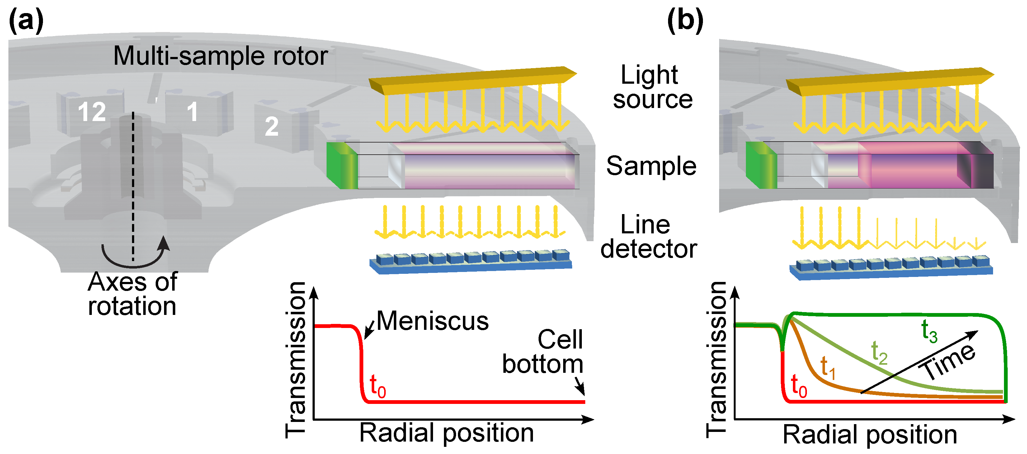
Figure 1. Scheme of an analytical centrifuge (AC) with a positioned measurement cell filled with a suspension: initial state at the start of centrifugation (a) and subsequent stages over time (b).
Make 08 00081 g001
Figure 2. Schematic representation of a Conditional (Wasserstein) Generative Adversarial Network. The generator (G) learns to produce real data from noise (z) and condition (c), while the discriminator (D) or critic (C) estimates the probability whether the data is real or fake.
Make 08 00081 g002
Figure 3. Schematic representation of a Conditional Variational Autoencoder. The encoder (E) maps the input data (X) and the condition (c) to a latent space representation and predicts the mean ( μ ) and variance ( σ ) of a Gaussian distribution. A sampled latent vector (z) is then passed to the generator (G), which aims to reconstruct the original data based on the initial condition.
Make 08 00081 g003
Figure 4. Representative experimental examples of the four classes: (a) sedimentation (SED), (b) flotation (FLT), (c) sedimentation–flotation combined behavior (SFL), and (d) other (OTH). Time evolution of profiles are color-coded from red to green.
Make 08 00081 g004
Figure 5. Grayscale images derived from the transmission profiles of four separation classes, (a) sedimentation (SED), (b) flotation (FLT), (c) sedimentation–flotation combined behavior (SFL), and (d) other (OTH). Radial position on the ordinate and time on the abscissa.
Make 08 00081 g005
Figure 6. Representative examples of simulated sedimentation profiles: (a) 2000 Sved, (b) 90,000 Sved, (c) 10,000 Sved and (d) 10,000 Sved with normalized radial position. Time evolution of profiles are color-coded from red to green.
Make 08 00081 g006
Figure 7. Schematic overview of the proposed Conditional Variational Autoencoder (Wasserstein) Generative Adversarial Network. The encoder (E) maps the input data (X) and the condition (c) to a latent space representation and predicts the mean ( μ ) and variance ( σ ) of a Gaussian distribution. A sampled latent vector (z) is then passed to the generator (G), which aims to reconstruct the original data based on the initial condition. Finally, the discriminator (D) or critic (C) estimates the probability whether the data is real or fake.
Make 08 00081 g007
Figure 8. Synthetic spatial- and time-resolved transmission profiles of liquid dispersions under centrifugation of 4 defined separation classes. (a) Sedimentation (SED), (b) Flotation (FLT), (c) Combination (SFL) and (d) Others (OTH). Time evolution of profiles are color-coded from red to green.
Make 08 00081 g008
Figure 9. Grayscale images derived from the transmission profiles of 4 separation classes based on the synthesized data, (a) Sedimentation (SED), (b) Flotation (FLT), (c) Combination (SFL), and (d) Other (OTH). Radial position on the ordinate and time on the abscissa.
Make 08 00081 g009
Figure 10. Effect of data pre-processing on transmission profiles. (a) Original data from a sedimentation class sample. (b) Pre-processed profile after profile reduction and intensity smoothing. Time evolution of profiles are color-coded from red to green.
Make 08 00081 g010
Figure 11. Loadings of the first three principal components (PC1–PC3) across the 512 latent features. Each panel (ac) shows a bar plot of the loading values for one PC, with the corresponding percentage of explained variance indicated in parentheses.
Make 08 00081 g011
Figure 12. First three principal components (PC1–PC3) of the ResNet34 latent feature space, shown as pairwise two-dimensional projections for the real dataset (ac) and the synthetic dataset (df). PC1, PC2, and PC3 capture 26%, 10.4%, and 5.6% of the total variance, respectively. Instances of sedimentation (SED) are shown as blue circles, flotation (FLT) as yellow squares, combined kinetics (SFL) as purple upright triangles, and other cases (OTH) as red diamonds.
Make 08 00081 g012
Figure 13. Comparison of the calculated sedimentation coefficient distributions of DBM (analytical solution) and the 5 trained generative networks with (a) an expected value of 21,875 Sved and (b) 78,125 Sved.
Make 08 00081 g013
Figure 14. Overview of (a) relative deviation and (b) coefficient of variation of the different generative networks for individual sedimentation coefficients.
Make 08 00081 g014
Table 1. Comparison of the classification performance of different models. Class-sensitive accuracies in %.
↑ Accuracy (%)
ModelSEDFLTSFLOTH
ResNet34-COL98.991.580.077.4
ResNet34-GRY99.389.077.861.3
LSTM99.379.728.90.0
GRU97.489.046.79.7
Transformer99.386.464.448.4
ResNet34-COL (FTN)98.591.577.890.3
ResNet34-GRY (FTN)99.386.471.158.1
LSTM (FTN)97.889.044.441.9
GRU (FTN)98.592.457.854.8
Transformer (FTN)98.990.775.667.7
BKC81.6 ± 7.621.7 ± 7.653.3 ± 32.155.0 ± 26.0
IKC98.3 ± 2.963.3 ± 16.380.0 ± 8.261.7 ± 2.9
AKC1007590100
Table 2. Comparison of the classification performance of different models and expert knowledge categories. The mean averaged accuracy, precision, recall, and F1-score values.
Model↑ Accuracy (%)↑ Precision (%)↑ Recall (%)↑ F1-Score (%)
ResNet34-COL93.7 ± 3.394.0 ± 3.393.6 ± 3.693.4 ± 3.5
ResNet34-GRY92.0 ± 1.992.6 ± 1.891.8 ± 2.291.6 ± 2.2
LSTM80.8 ± 3.376.0 ± 4.580.8 ± 3.476.4 ± 3.8
GRU84.4 ± 1.383.4 ± 4.984.6 ± 1.181.6 ± 1.7
Transformer89.2 ± 1.889.0 ± 1.989.0 ± 1.688.2 ± 1.9
ResNet34-COL (FTN)94.2 ± 3.194.6 ± 2.994.2 ± 3.393.8 ± 3.3
ResNet34-GRY (FTN)90.5 ± 2.490.8 ± 2.690.2 ± 2.389.8 ± 2.4
LSTM (FTN)86.6 ± 1.786.6 ± 1.586.6 ± 1.585.4 ± 2.1
GRU (FTN)90.1 ± 2.490.4 ± 2.590.0 ± 2.589.0 ± 2.9
Transformer (FTN)92.4 ± 0.892.8 ± 0.492.2 ± 0.892.0 ± 0.7
BKC52.9 ± 11.258.0 ± 23.752.9 ± 24.752.1 ± 20.2
IKC75.8 ± 4.276.1 ± 9.775.8 ± 15.975.3 ± 11.6
AKC91.391.691.391.0
Table 3. Mean Squared Error (MSE), Root Mean Square Error (RMSE), Mean Absolute Error (MAE), and R2 results of different regression models.
Model↓ MSE (Sved2)↓ RMSE (Sved)↓ MAE (Sved)↑ R2
ResNet34-COL1,842,579135710210.998
ResNet34-GRY1,439,34012009870.998
LSTM98,463,792992361210.882
GRU81,283,280901651120.902
Transformer2,691,006164015090.997
Table 4. Comparison of the regression performance of different models predicted with ResNet34. Mean Squared Error (MSE), Root Mean Square Error (RMSE), Mean Absolute Error (MAE), R2, and Fréchet Inception Distance (FID) results for sedimentation profiles synthesized from cWGAN, cWGAN-PhysC, cVAE, cVAE-PhysC, cVAE-GAN and cVAE-GAN-PhysC.
Model↓ MSE (Sved2)↓ RMSE (Sved)↓ MAE (Sved)↑ R2↓ FID
cWGAN7,709,994277625300.990220
cWGAN-PhysC8,080,177284223560.990422
cVAE9,930,741315126440.988540
cVAE-PhysC3,123,440176713390.996150
cVAE-GAN6,100,652246920450.993280
cVAE-GAN-PhysC14,211,472376929390.983912
Disclaimer/Publisher’s Note: The statements, opinions and data contained in all publications are solely those of the individual author(s) and contributor(s) and not of MDPI and/or the editor(s). MDPI and/or the editor(s) disclaim responsibility for any injury to people or property resulting from any ideas, methods, instructions or products referred to in the content.