Model-Aware Automatic Benchmark Generation with Self-Error Instructions for Data-Driven Models

Abstract

The growing number of domain-specific machine learning benchmarks has driven methodological progress, yet real-world deployments require a different evaluation approach. Model-aware synthetic benchmarks, designed to emphasize failure modes of existing models, are proposed to address this need. However, evaluating already well-performing models presents a significant challenge, as the limited number of high-quality data points where they exhibit errors makes it difficult to obtain statistically reliable estimates. To address this gap, we proposed a two-step benchmark construction process: (i) using a genetic algorithm to augment the data points where data-driven models exhibit poor prediction quality; (ii) using a generative model to approximate the distribution of these points. We established a general formulation for such benchmark construction, which can be adapted to non-classical machine learning models. Our experimental study demonstrates that our approach enables the accurate evaluation of data-driven models for both regression and classification problems.

1. Introduction

The rapid growth of domain-specific machine learning benchmarks has been instrumental in driving methodological progress: standard datasets and evaluation protocols enable rigorous, reproducible comparison of novel model architectures and training strategies against established state-of-the-art baselines. However, as artificial intelligence systems are increasingly deployed across diverse industrial and applied settings, different evaluation needs have emerged.

In many real-world deployments, practitioners already operate high-quality models that perform well on average but fail in a small, application-critical subset of cases. When presented with a candidate replacement, the primary requirement is not only higher overall accuracy but, more importantly, reliable improvement precisely on those rare failure modes. Conventional benchmark datasets, designed to discriminate among newly proposed models using abundant labeled examples, are poorly suited to this scenario, as the number of documented failure cases for a well-tuned model is intrinsically small. Therefore, obtaining sufficient high-quality data for statistical comparisons of model quality remains challenging.

To address this gap, we propose the design of model-aware synthetic benchmarks that (i) are synthetic because real-world failure examples are too scarce to deliver statistically meaningful interval estimates, and (ii) use “self-error” instructions (i.e., conditioned on the model’s observed behavior) because the benchmark dataset must deliberately emphasize the regions of input space where the deployed system underperforms. This paradigm shifts evaluation from objective, model-agnostic competition to targeted, diagnostic synthesis problems whose goals are to produce reliable, task-relevant estimates of relative improvements. Recent work on generation-centric benchmarking has highlighted both the promise and pitfalls of these approaches: while synthetic benchmark datasets can unify assessment across methods and domains, they can also inherit biases from the generative or evaluation models used in their construction, thereby affecting the objectivity of comparisons [1,2,3].

Implementing such a synthetic, model-aware benchmark dataset gives rise to two principal technical challenges. First, the problem is fundamentally inverse: we seek to synthesize inputs that reveal or amplify specific failure modes of an existing discriminative model based solely on its observed outputs. This inverse formulation increases sensitivity to noise and model idiosyncrasies and requires principled regularization and uncertainty quantification.

Second, any generator used to produce benchmark dataset cases is itself a model and therefore a possible source of systematic artifacts; evaluation procedures must therefore separate improvements attributable to genuine robustness from those produced by generation biases or overfitting to generator artifacts. The prior literature on benchmark datasets for generative systems and on the evaluation of model-generated data highlights these risks and motivates careful experimental design and defensive controls.

Automatic benchmarks are also essential in AutoML. The implementation of automatic model structure creation requires comparisons of resulting instances, which can be effectively achieved through automated benchmarking [4,5,6]. This type of benchmarking is crucial for automated systems, as it enables decision-making processes regarding the use or development of models without human intervention.

Our contributions are as follows:

(i)

We formalize the task of model-aware automatic benchmark dataset generation using self-error instructions for classical machine learning models.

(ii)

We propose a two-stage pipeline for benchmark dataset generation, using a genetic algorithm to augment the bad prediction points and a generative model to approximate their distribution.

(iii)

We conduct several experiments to demonstrate the applicability of our benchmark on both synthetic and real-world datasets for regression and classification problems.

2. Related Works

The conventional approach to benchmark dataset construction involves using high-quality datasets tailored to specific tasks [7]. Each benchmark dataset covers a limited range of data properties, sometimes covering multiple properties [1,8]. However, this approach is inherently limited because it does not directly address the quality of the models themselves. A sufficiently advanced model will eventually achieve 100% quality on a predefined benchmark dataset. This occurs because models are continuously being improved, and past tasks may no longer pose significant challenges for more sophisticated models. Additionally, benchmark data leakage into the training sample is a potential concern.

Consequently, new benchmark datasets are created, and researchers develop more complex tasks. Nevertheless, the rapid advancement of large language models (LLMs) presents challenges in increasing the complexity of tasks [9]. Recent competitions have demonstrated that contemporary LLMs can solve previously unexplored Olympiad programming tasks while simultaneously achieving high-quality performance [10,11,12].

The primary objective of this article is to establish benchmark datasets for classical machine learning tasks. Notably, the work in [13] has created a benchmark for evaluating generative models based on time series data. Utilizing a substantial dataset, various windows are computed, and models are then tested within these windows to assess their generation quality and generalization capabilities. Another relevant work concerns the development of a synthetic benchmark dataset for interpretable machine learning [3]. Both works generate datasets that can be used to evaluate models. However, the challenge of evaluating model quality in real-time based on the model’s performance remains an open question.

Our approach is also related to the concept of error-driven data augmentation, where models focus on poor predictions or generation and attempt to incorporate this information into subsequent iterations. Recent works in this area include applications to LLMs [14,15].

An interesting analogy with our approach can be drawn from works [16,17]. In these works, authors construct ensembles based on a specific measure of diversity. The greater the diversity of individual models within the ensemble, the better the overall performance of the ensemble. This analogy suggests that we aim to identify such data to enhance the quality of the entire benchmark while simultaneously considering the importance of diversity in the data selection process. An illustrative example is provided in [18], which demonstrates the construction of an ensemble using a genetic algorithm. In our case, we use a genetic algorithm to generate a benchmark that comprehensively covers a wide range of scenarios relevant to the current model.

Finally, our approach is directly related to synthetic data. The construction of synthetic benchmark datasets is actively studied by researchers [2,19,20]. This data approach enables adapting the data to meet the specific requirements of model quality control. For instance, source benchmarks can be enriched with various additions related to specific tasks within a particular field of knowledge.

3. General Problem Formulation

Let $\mathcal{D}={\{X_i,y_i\}}_{i = 1}^N$ be a dataset that comprises input and output variables. Assume that F is an operator that transforms input variables into output variables. This operator defines the data-driven model $y=F\left(X\right)$. The variable X can encompass any type of variable (numerical, ordinal, or nominal) and can be of any dimension d. We define such a space as ${\mathcal{X}}^d$. The output variable can also be of any dimension and represent not only numerical targets but also categorical data.

Let G be another operator that we intend to evaluate. We assume that G is a superior model. However, if the general quality of F and G is comparable, it becomes challenging to accurately assess the overall performance of the new model G.

A commonly employed technique for this purpose is cross-validation. However, it is crucial to recognize that the cross-validation estimate is limited by the quality of the data it is based on. If the dataset is small, noisy, or does not adequately represent the real world, the cross-validated score may provide an accurate estimate of performance on limited or poor data. Nevertheless, it does not provide a comprehensive evaluation of the model or algorithm’s capabilities in a broader context.

In this context, automatic benchmarking methods emerge as a solution to this problem. We can generate a new dataset $\tilde{\mathcal{D}}$ based on the existing one, incorporating any necessary modifications. One approach involves using the data points where the model F exhibits unsatisfactory performance.

Let F be a pretrained model. We can separate the dataset $\mathcal{D}$ into two disjoint sets $\mathcal{D}={\mathcal{D}}_0\bigcup {\mathcal{D}}_b$. The set ${\mathcal{D}}_0$ contains the data points where the operator F makes accurate predictions, while the set ${\mathcal{D}}_b$ contains the data points where the predictions deviate from the target variable y. We designate the points $X_b\in {\mathcal{X}}^d$ as “bad” points and denote them with the subscript b. The corresponding targets are denoted as $y_b$.

The criterion for partitioning the dataset $\mathcal{D}$ into disjoint subsets is the operator K applied to data points ${\mathcal{D}}_b=K(\mathcal{D};F)$. This operator K (condition) is defined phenomenologically, based on empirical observations of the operator F’s behavior. For example, in a regression problem, we can partition the dataset $\mathcal{D}$ based on the mean squared error. In general, for data-driven models, it can be defined as

$$K(\mathcal{D};F)\equiv K\left(\right\{X,y\};F)=\left\{\right(X,y\left)\right|h\left(F\right(X),y)\le (\ge /</>)\alpha \},$$

(1)

where h represents the function that quantifies the error between the prediction and the target value, and $\alpha$ serves as the threshold for selecting the bad points.

The objective is to evaluate the model G, but the evaluation criteria remain the same as for F, and we also assume that F is a sufficiently effective model. Consequently, $|{\mathcal{D}}_0|\gg |{\mathcal{D}}_b|$. This implies that we were unable to compare the models on bad points and obtain statistically significant estimations.

Thus, we can use augmentation and generation techniques to modify ${\mathcal{D}}_b$ and construct the new dataset $\hat{\mathcal{D}}={\mathcal{D}}_b\bigcup \tilde{\mathcal{D}}$ for evaluation purposes, where $\tilde{\mathcal{D}}$ is the synthetic dataset.

It is important to note that our approach does not categorize non-typical data points as outliers but rather as challenging to predict, particularly in the context of real-world data. We do not discard such points; instead, we use them to rigorously test the model for which we are establishing a benchmark dataset. This approach contrasts with approaches related to robust statistics, which were investigated in the works of Peter J. Huber [21]. In other words, ${\mathcal{D}}_b$ generally represents a different population, distinct from ${\mathcal{D}}_0$. However, in our setting, we believe that this data is valuable, but there are too few instances to train or test the model efficiently. Consequently, we need to augment the data to obtain enough instances for training and testing.

The synthetic dataset $\tilde{\mathcal{D}}$ is constructed in two distinct stages. The first stage involves an augmentation process facilitated by a genetic algorithm. This augmentation process aims to introduce random perturbations to the target points y, thereby increasing the variability of the data. We denote the perturbed targets as $y_{ga}$. This stage samples points $X_{ga}$ that are close to the initial bad points $X_b$, but with several random modifications applied to increase the dataset’s size and facilitate the effective use of generative models.

In genetic algorithms, the loss function is used to generate points from the existing dataset while introducing a larger prediction error. However, since it is possible to find arbitrarily distant points where the error will be substantial, the augmentation task loses its significance. Consequently, a regularizer is also introduced to ensure the quality and consistency of the generated points (Section 4.3).

The second stage is used to learn the distribution of bad points and effectively sample new bad points from it. For this purpose, we employ a variational autoencoder, which first encodes the augmented points $X_{ga}$ into a latent space and then samples new bad points $\tilde{X}$ from the latent space (Section 4.4).

4. Automatic Benchmark Model

4.1. General Pipeline for Regression Problems

Figure 1 illustrates the general pipeline for benchmark dataset construction for regression models.

First, we partition the data into training $\{X_{tr},y_{tr}\}$ and testing sets $\{X_{te},y_{te}\}$. Next, we train transformations to normalize numerical attributes and encode categorical attributes. For example, min-max normalization can be applied to numerical features, while ordinal encoding is suitable for categorical data. The trained transformations should be subsequently applied to the test set. Then, we train the baseline model F on the training sample and evaluate the model’s performance on the test sample.

In the next step, we identify the bad instances of the baseline model within the test dataset using a specified metric and threshold value $\alpha$:

$${\mathcal{D}}_b=K(\{X_{te},y_{te}\};F)=\left\{(X_{te},y_{te})\right|{(F\left(X_{te}\right)-y_{te})}^2\ge \alpha \}.$$

(2)

Then, we augment these bad examples to enhance the dataset’s variability, thereby expanding the training set for the subsequent generative phase.

For the augmentation process, we use a genetic algorithm due to its favorable characteristics of flexibility in individual identification and its inherent variability in the search process, which provides rapid convergence to optimal points. We also developed custom mutation and crossover operators, as well as a fitness function. The details of this genetic algorithm are presented in Section 4.3.

The points we obtain after augmentation with a genetic algorithm are denoted as $\{X_{ga},y_{ga}\}$. These points also include the bad points $\{X_b,y_b\}$, but with additional augmented examples. Next, we take these points and train a generative model on them. This generative model produces synthetic data points $\{\tilde{X},\tilde{y}\}$. The description of the generative model is presented in Section 4.4.

In the final step, we evaluate the new model g on the synthetic dataset, and we repeat the entire process multiple times, starting with different splits of the training set $X_{tr}$ and test set $X_{te}$.

4.2. General Pipeline for Classification Problems

Our approach can also be adapted to classification problems. In the context of classification problems, we can employ the notation $\{X,y\}$, where $y\in \mathbb{N}$. This notation allows us to identify the instances that are considered “bad” by associating them with a threshold value $\alpha$.

Consider a binary classification problem, where the label $y\in \{0,1\}$. The model’s output $F\left(X\right)$ is the probability p of label <<1>>. We define bad points as follows:

(i)

If $y=1$, then bad points are those for which $p\le \alpha$.

(ii)

If $y=0$, then bad points are those for which $(1-p)\le \alpha$.

In this case, the threshold $\alpha$ should be approximately equal to the probability cutoff threshold for classification, which is typically set at $0.5$ in standard practice. In terms of the operator K, this can be written as

$${\mathcal{D}}_b=K(\{X_{te},y_{te}\};F)=\left\{(X_{te},y_{te})\right|F\left(X_{te}\right)\le \alpha ,\mathrm{if}{y}_{te}=1\}\bigcup \left\{(X_{te},y_{te})\right|(1-F\left(X_{te}\right))\le \alpha ,\mathrm{if}{y}_{te}=0\}.$$

(3)

Thus, our focus is on the points where the model exhibits the lowest level of confidence in its prediction capabilities. These are the points where the model demonstrates weaknesses, and in these regions, we intend to evaluate the new model’s performance, assessing whether it can yield improvements compared to the baseline model.

For multi-label classification problems, the operator K is reformulated as,

$${\mathcal{D}}_b=K(\{X_{te},y_{te}\};p_1,\dots ,p_L)=\left\{(X_{te},y_{te})\right|p_1\le \alpha ,\mathrm{if}{y}_{te}=1\}\bigcup \cdots \bigcup \left\{(X_{te},y_{te})\right|p_L\le \alpha ,\mathrm{if}{y}_{te}=L\},$$

(4)

where $p_1,\dots ,p_L$ represent the probabilities obtained by the model F for the corresponding labels $y\in \{1,\dots ,L\}$. In the general case, it is also possible to consider different threshold levels for each label, $\{{\alpha }_1,\dots ,{\alpha }_L\}$.

4.3. Genetic Algorithm

4.3.1. Formulation for Regression Problems

A genetic algorithm was employed for several reasons. First, our search space is extensive, particularly due to the increasing number of features. Second, our search space encompasses both discrete and numerical attributes simultaneously. Thus, we must discover new feature values based on the nature of the data. This optimization problem lacks differentiability. Genetic algorithms also possess general advantages, such as avoiding local optima through population diversity and effectively managing black-box or non-linear models.

To obtain the augmented points $X_{ga}$, we treat each instance as a unique individual. Each instance comprises both discrete and numerical attributes. The numerical attributes are normalized to the range $[0, 1]$, and the categorical attributes are transformed into numerical integer representations using the ordinal encoder (OrdinalEncoder [22]). This numerical encoding enables the accurate application of the regression model.

A distinction exists between ordinal and nominal categorical features. While the ordinal encoder is well-defined for ordinal attributes, it is not compatible with nominal features because ordinal labels have a specific order, whereas nominal features do not. However, for simplicity in genetic operators, we used the ordinal encoder for the entire set of categorical attributes.

The augmentation process comprises two distinct components. First, we introduce small random perturbations into the target $y_b$. Given that we determined the min–max normalization parameters on the training data to prevent data leakage to the test set, the test set may contain values that are not precisely within the range $[0, 1]$. We denote the minimum and maximum values as $y_{min}$ and $y_{max}$, respectively. For the perturbations, we use a normal random variable with appropriate bounds. That is,

$$y_{ga}\left(i\right)=max\{y_{min},min\{y_{max},y_b\left(i\right)+\xi \}\},$$

(5)

where $\xi \sim \mathcal{N}(0,{\sigma }_{\xi }^2)$.

Second, for each iteration of point augmentation, we employ the genetic algorithm with the following fitness function. The fitness function, denoted as $\mathcal{L}$, serves as the objective that we aim to optimize. The function $\mathcal{L}$ represents the difference between the augmented value $y_{ga}$ and the predicted value $F\left(X_{ga}\right)$. In this context, the changes only concern the individuals $X_{ga}$. The goal is to maximize their difference, as we want to find other bad points. However, as we can find any combination of attributes in individuals and can increase the individuals’ values to infinity, we incorporate the regularization. This regularization has the form ${(X_b\left(i\right)-X_{ga}\left(i\right))}^2\to 0$. For flexibility purposes, we also add a multiplier $\kappa \in [0,1]$ for the first fitness component.

Finally, the fitness function equals

$$\mathcal{L}\left(i\right)=\kappa {(y_{ga}\left(i\right)-F\left(X_{ga}\left(i\right)\right))}^2-{\displaystyle \frac{1}{d}}\sum _{j = 1}^d{(X_{ga}^j\left(i\right)-X_b^j\left(i\right))}^2.$$

(6)

Next, we define the population and its representation. In our task, each population individual is a dataset instance that encompasses both categorical and numerical data. The population size can initially be large to increase variability and improve convergence. We generate the population by randomly repeating individuals. For this purpose, we randomly sample points from the unique set of values for each attribute. This ensures that the population closely resembles the initial points in $X_{te}$. Additionally, for numerical attributes, it is also possible to sample points uniformly from the range $[y_{min},y_{max}]$. This provides greater flexibility to the population, but it can also yield inaccurate results, as only certain parts of the range $[y_{min},y_{max}]$ may be included in $X_{te}$.

The last two components of genetic algorithms include the mutation and crossover operators. We implement these operators, taking into account the specifics of our task. Specifically, categorical features cannot mutate in the same way as continuous ones. For categorical features, we employ the same sampling technique used during the population creation phase. Specifically, we randomly select a category value from the list of unique values present in the column.

For numerical features, we introduce the concept that if a feature positively influences a target variable, then in a scenario requiring an increase in the target value, it is necessary to simultaneously increase the positively influencing features. Nevertheless, certain attributes may have a positive impact, while it may be necessary to reduce the values of these attributes and simultaneously increase those that exert a stronger influence. This additional idea for numerical attributes can enhance the search for the optimal individual corresponding to the $y_{ga}$.

Algorithm 1 illustrates the comprehensive steps involved in the mutation operator for both categorical and numerical features. The input is the individual $\mathcal{I}$, where the first $M_c$ values correspond to categorical features. The weights $\omega$ represent the influence of each attribute on the target variable. These weights are determined using the coefficients obtained from linear regression. The parameter $\zeta$ identifies the direction of change, $p_m$ is the probability of mutation, and $s_m$ is the mutation strength.

The parameter $\zeta$ is the target direction that is identified as follows: if $y_{ga}\ge F\left(X_b\right)$, then $\zeta =1$, indicating that we should increase the prediction value; if $y_{ga}<F\left(X_b\right)$, then $\zeta =-1$.

When the ${\omega }_i\ge 0$ (positive influence of attribute i on the target) and $\zeta \ge 0$, the direction of change for the variable equals $\hat{\zeta }=1$. Similarly, when ${\omega }_i\le 0$ and $\zeta \le 0$, the direction of change is also $\hat{\zeta }=1$. This implies that we need to change the variable in the same direction as $\zeta$ value. However, when ${\omega }_i\ge 0, \zeta \le 0$ and ${\omega }_i\le 0, \zeta \ge 0$, we need to change the variable in the opposite direction, resulting in $\hat{\zeta }=-1$.

Finally, we sample the random normal variable $\kappa$ and modify the value of the individual using the rule $\hat{\zeta }·\left|\kappa \right|$. Additionally, it is crucial to consider the domain region. In extreme scenarios, we can allow values to be outside the domain $[y_{min},y_{max}]$ to encompass a broader range of potential values.

Algorithm 1 Mutation operator.

Input: $\mathcal{I}$, $\omega$, $\zeta$, $p_m$, $s_m$ Require: $p_m,s_m\in [0,1]$, $\zeta \in \{-1,1\}$ Return: $\tilde{\mathcal{I}}$   1: $\tilde{\mathcal{I}}\leftarrow \mathcal{I}$   2: for $i\leftarrow 0$ to $\left|\mathcal{I}\right|$ do   3:      Sample random variable $\eta$ from the uniform distribution $\mathcal{U}[0,1]$   4:      if $\eta <p_m$ then   5:          if $i<M_c$ then   6:             ${\tilde{\mathcal{I}}}_i\leftarrow$ sample from the column $X^{\left(i\right)}$   7:          else   8:             if ${\omega }_i·\zeta \ge 0$ then   9:                 $\hat{\zeta }\leftarrow 1$ 10:             else 11:                $\hat{\zeta }\leftarrow -1$ 12:             end if 13:             $z\leftarrow \hat{\zeta }·\left|\kappa \right|$, where $\kappa \sim \mathcal{N}(0,s_m)$ 14:             ${\tilde{\mathcal{I}}}_i\leftarrow max\{y_{min},min\{y_{max},{\tilde{\mathcal{I}}}_i+z\}\}$ 15:          end if 16:      end if 17: end for

The crossover operator provides mixing of individuals. For instance, two-point crossover or uniform crossover [23] can be implemented for categorical attributes. In this case, the values of categorical features are randomly selected from a set of unique feature values and are not blended across other categorical features. For numerical attributes, it is possible to use any blending technique while preserving the bounds.

For the selection process, we employ the standard tournament selection algorithm [24] with a tournament size of 3. This approach involves selecting the three best individuals in the population at each optimization step. All genetic operators were implemented using the DEAP framework [25].

4.3.2. Formulation for Classification Problems

The method for identifying augmented points $X_{ga}$ is analogous to that employed in regression problems. The same mutation and crossover operators are used. The distinction lies in the fitness function.

In this case, we cannot introduce random perturbations to the target variable y because it is binary. Consequently, we employ a distinct type of augmentation; specifically, we randomly modify the class label with a probability of $p_{\xi }$. The objective function negatively impacts the model’s prediction, similar to the regression case. However, in this scenario, the deterioration is revealed as a reduction in the model’s confidence in predicting the positive class. That is,

$$\mathcal{L}\left(i\right)=-\kappa F\left(X_{ga}\left(i\right)\right)-{\displaystyle \frac{1}{d}}\sum _{j = 1}^d{(X_{ga}^j\left(i\right)-X_b^j\left(i\right))}^2,$$

(7)

where $\kappa \in [0,1]$ is a multiplier.

4.4. Generative Model

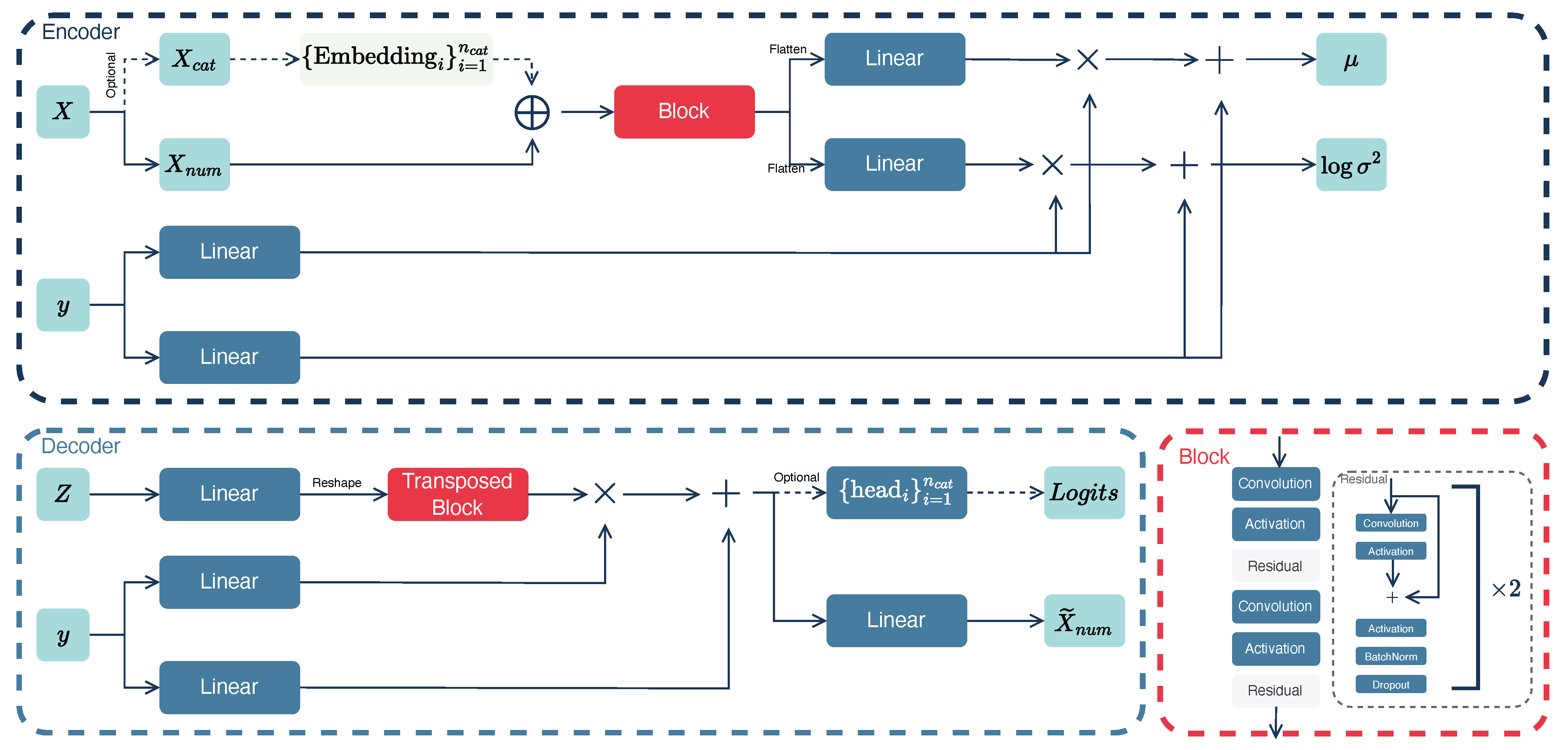
In this study, we employ a variational autoencoder to generate new instances of bad points. The architecture of the autoencoder is presented in Figure 2.

The encoder component of the autoencoder receives both the features and the target. The features can be processed in two distinct ways. If categorical features are present, we apply an embedding layer to each categorical feature $i\in \{1,\dots ,n_{cat}\}$. This embedding is a matrix whose size equals the number of different categories in feature column i multiplied by the embedding vector dimension. Subsequently, these embeddings are concatenated with the numerical features. If there are no categorical features, only numerical attributes are used.

Next, we implement a block architecture (red box) that comprises multiple convolutional layers (Convolution) and residual blocks (Residual). Following each convolution operation, we employ a non-linear activation function (Activation). These convolution transformations are used to control the number of channels. The residual block (gray box) employs the same convolutions and activations but with residual connections. This involves adding the outputs from the previous layer to the current layer’s output.

Then, we flatten the tensors into a one-dimensional vector and apply two linear layers to compute the mean and the logarithm of the variance of the latent normal distribution. Notably, we incorporate target information into this process by using the linear modulation technique known as FiLM [26]. Specifically, we feed the target y into linear layers and multiply and sum it with the output of the main network flow. In classification problems, the target variable y is binary, taking values of 0 or 1. To address this, we employ an embedding layer.

The decoder architecture starts by sampling the latent vector Z from the normal distribution $\mathcal{N}(\mu ,e^{log{\sigma }^2})$. For this, we use the standard reparametrization trick. Specifically, we sample the random variable $\epsilon$ from the standard normal distribution $\mathcal{N}(0,I)$ and apply the linear transformation $\mu +\epsilon \ast e^{{\displaystyle \frac{1}{2}}log{\sigma }^2}$.

Next, we employ linear projection to resize the tensor appropriately for input into the convolutional layers within the transposed convolution block. This block retains the same activations and residuals but uses transposed convolutions instead. After that, we apply linear modulation, similar to the encoder, to the output of the transposed convolution block.

Finally, if the data include categorical variables, the optional branch is used. In this branch, we employ heads, which are represented as linear projections for each category individually. Specifically, each head maps to the $Logits$ vector with size equal to the number of unique values in column i. The latent representation of numerical features is processed with a linear projection whose size equals the number of numerical variables.

After training the generative model, we sample the latent vector Z and use the targets y to generate the synthetic data $Logits$ and ${\tilde{X}}_{num}$. To construct the complete synthetic dataset $\tilde{X}$, we transform $Logits$ through the softmax function and use the argmax function to extract the categorical data ${\tilde{X}}_{cat}$. Consequently, the final synthetic data $\tilde{X}$ are formed by concatenating both components: $\tilde{X}={\tilde{X}}_{cat}\oplus {\tilde{X}}_{num}$. The synthetic dataset including targets equals $\tilde{D}=\tilde{X}\oplus \tilde{y}$, where $\tilde{y}$ can represent targets $y_b$ from the initial bad data or augmented targets $y_{ga}$ after the genetic algorithm.

5. Experimental Study

5.1. Data Description

We conducted experiments with three datasets: a synthetic toy dataset and two real-world tabular datasets.

The toy dataset comprises two numerical features and a single target variable. We randomly sampled points within the square $[0,1]\times [0,1]$. Then, we produced target values by applying the linear transformation $y=2x_1+3x_2+7+ϵ{\sigma }_{\epsilon }$, where $ϵ\sim \mathcal{N}(0,1)$ and ${\sigma }_{\epsilon }=0.1$ (blue points in Figure 3a). However, for the regions $[0.1,0.3]\times [0.6,0.8]$ and $[0.6,0.8]\times [0.3,0.5]$, we sampled points with a different kind of relationship: $y=2x_1+x_1^2-8x_2-4+ϵ{\sigma }_{\epsilon }$ (red points in Figure 3a). We sampled one thousand points with a train–test ratio of 8:2.

For illustrative purposes, we sampled points from a uniform distribution. Nevertheless, it is important to recognize that in practical scenarios, the points correspond to a more complex multidimensional distribution characterized by a substantial number of modes.

We use the real-world dataset that provides information on apartment prices in Moscow. This dataset comprises 26 attributes and a single target variable. The total number of observations equals 253,000. The target variable represents the price per square meter. The dataset includes one categorical variable, and the remaining attributes are numerical.

The numerical attributes describe the characteristics of the apartments, including their proximity to schools, subway stations, the number of floors in the building, parking availability, and other building-related attributes. The categorical feature represents the building’s class, such as business, economy, and comfort. The train–test ratio equals 8:2.

We also use the publicly accessible real-world dataset, accessible via the provided link (https://www.kaggle.com/datasets/mohankrishnathalla/diabetes-health-indicators-dataset, accessed on 17 November 2025), to assess the performance of our benchmark model on classification problems. This dataset encompasses 100,000 observations, each representing various medical indicators. The target variable is a binary label, where 1 signifies the presence of diabetes and 0 indicates its absence. We select 12 features from the comprehensive feature set, including gender, ethnicity, income level, insulin level, age, smoking status, BMI, and others. The final set of selected features comprises four categorical and eight numerical features.

5.2. Evaluation Scores

To evaluate the quality of models based on various data, we use the Mean-Squared Error (MSE), the Symmetric Mean Absolute Percentage Error (SMAPE), and the Wasserstein distance. The SMAPE is a forecasting accuracy measure that calculates the average percentage error between predicted and actual values. Unlike the standard Mean Absolute Percentage Error (MAPE), which can be biased towards over- or under-forecasting, the SMAPE employs a symmetric formula to mitigate this issue. Its definition is as follows:

$$\mathrm{SMAPE}(y,\hat{y})={\displaystyle \frac{2}{N}}\sum _{i = 1}^N{\displaystyle \frac{|{\hat{y}}_i-y_i|}{|{\hat{y}}_i|+|y_i|}},$$

(8)

where ${\hat{y}}_i$ is the predicted value, $y_i$ is the actual value, and N is the number of instances in the test set. Accordingly, when dealing with augmented data, the actual value $y_i$ is replaced by $y_{ga}\left(i\right)$, and the predicted value ${\hat{y}}_i$ is replaced by $F\left(X_{ga}\left(i\right)\right)$, where F is the corresponding regression model. For the synthetic data, $y_i={\tilde{y}}_i$ and ${\hat{y}}_i=F\left(\tilde{X}\left(i\right)\right)$.

The Wasserstein distance serves as a quantitative measure of similarity between synthetic and real-world data. In this context, it is used to illustrate the resemblance between $\tilde{X}$ and $X_{ga}$.

The Wasserstein distance (1-Wasserstein distance) quantifies the minimal cost associated with transforming one probability distribution into another. It is determined by identifying the optimal transport plan, which represents the most efficient method for relocating mass from one distribution to another. In the one-dimensional case, the Wasserstein distance is equivalent to the area between the cumulative distribution functions (CDFs) of the two distributions. The optimal value of the Wasserstein distance is 0.

$$\mathrm{Wasserstein}\mathrm{distance}(u,v)=\underset{\pi \in \Gamma (u,v)}{inf}{\int }_{\mathbb{R}\times \mathbb{R}}|x-y|d\pi (x,y),$$

(9)

The set $\Gamma (u,v)$ consists of probability distributions on $\mathbb{R}\times \mathbb{R}$ whose marginals are u and v. For a specific value x, $u\left(x\right)$ represents the probability of u occurring at position x, and the same applies to $v\left(x\right)$.

For classification problems, we use the standard $F_1$ score, which is the harmonic mean of the precision and recall.

$$F_1(y,\hat{y})={\displaystyle \frac{2\times \mathrm{precision}(y,\hat{y})\times \mathrm{recall}(y,\hat{y})}{\mathrm{precision}(y,\hat{y})+\mathrm{recall}(y,\hat{y})}},$$

(10)

where the precision is defined as the ratio of true positive results to the total number of samples predicted to be positive, encompassing both correctly and incorrectly identified samples. Recall, on the other hand, is the ratio of true positive results to the total number of samples that should have been identified as positive. The $F_1$ score, a symmetric measure, effectively combines both precision and recall into a single metric. The optimal $F_1$ score is 1, indicating perfect precision and recall, while a score of 0 signifies the absence of both.

Additionally, we use the ROCAUC score, which represents the area under the receiver operating characteristic (ROC) curve. The optimal value of $\mathrm{ROCAUC}(y,\hat{y})$ is 1, while the worst-case scenario corresponds to 0.

5.3. Toy Example

Figure 3 illustrates the entire workflow of the benchmark pipeline for the toy example. First, we identify specific regions where the target variable deviates from the linear relationship in contrast to the other points within the square (Figure 3b). For this purpose, we use the threshold $\alpha =0.2$.

For the baseline model F, we employ a linear regression model with $L_2$ regularization. For the model G, we use a gradient boosting approach with 100 trees and a maximum depth of 3.

Next, we use the genetic algorithm to augment the initial target values. In general, we must assume the continuity of the data points. That is, the neighboring points should have correspondingly close target values. Otherwise, the convergence can be severely hindered. Augmented points are denoted in green in Figure 3c.

Figure 3d shows the predictions achieved by the regression model on both bad $X_b$ (red points) and augmented $X_{ga}$ data points (green points). The ideal scenario is represented by an identity line, signifying that the predictions accurately align with the target values derived from the original data. For augmented data points, the target remains the original target with the random perturbation introduced earlier. Thus, it is evident that the regression model exhibits significant challenges in predicting bad data points (which prompted their selection). However, we are also able to generate new data points surrounding the existing ones, maintaining the same property that the model struggles to capture in its predictions.

The blue points in Figure 3d represent the predictions for the remaining points in the test sample. As is evident, the model performs well on these points, as they are generated considering the linear relationship between features and the target.

The final step involves identifying the distribution of the obtained augmented points. To achieve this, we use the variational autoencoder to learn the complex data distribution and subsequently generate new adversarial points from that distribution. The new points are denoted in purple in Figure 3e. We generated five times more points than after the augmentation step.

We also demonstrate the baseline regression model’s results on these points in comparison to the new regression model. It is evident that gradient boosting handles augmented data points more effectively than linear regression. Linear regression concentrates all predictions in one area and cannot process new data points correctly. However, gradient boosting, although it does not perfectly follow the identity line, still handles different points and regions differently, making predictions closer to the target.

The quantitative results are presented in

Table A1. Comparison of prediction model results on the synthetic benchmark dataset. We repeat the train–test split procedure 31 times and execute the entire pipeline on these distinct splits. For statistical significance, we provide the standard deviation.

Model	Percent of Bad Points in ${\mathit{X}}_{\mathbf{te}}$, %	Data	MSE (MEAN ± STD)	SMAPE (MEAN ± STD)	Wasserstein Distance (MEAN ± STD)
Baseline model	10	$X_b$	$0.3655\pm 0.1099$	$1.1391\pm 0.3119$	—
		$X_{ga}$	$0.3761\pm 0.1134$	$1.1411\pm 0.3127$	—
		$\tilde{X}$	$0.3760\pm 0.1133$	$1.1412\pm 0.3127$	$0.0154\pm 0.0026$
	56	$X_b$	$0.1271\pm 0.0302$	$0.4921\pm 0.0900$	—
		$X_{ga}$	$0.1322\pm 0.0317$	$0.4923\pm 0.0906$	—
		$\tilde{X}$	$0.1314\pm 0.0318$	$0.4914\pm 0.0907$	$0.0114\pm 0.0025$
	75	$X_b$	$0.1133\pm 0.0073$	$0.5907\pm 0.0349$	—
		$X_{ga}$	$0.1443\pm 0.0082$	$0.6312\pm 0.0320$	—
		$\tilde{X}$	$0.1427\pm 0.0084$	$0.6300\pm 0.0326$	$0.0127\pm 0.0029$
Model for comparison	10	$X_b$	$0.0253\pm 0.0357$	$0.2229\pm 0.1485$	—
		$X_{ga}$	$0.0972\pm 0.0546$	$0.4437\pm 0.1784$	—
		$\tilde{X}$	$0.0738\pm 0.0590$	$0.3969\pm 0.1827$	$0.0154\pm 0.0026$
	56	$X_b$	$0.0113\pm 0.0117$	$0.0779\pm 0.0491$	—
		$X_{ga}$	$0.0798\pm 0.0225$	$0.2555\pm 0.0629$	—
		$\tilde{X}$	$0.0801\pm 0.0226$	$0.2609\pm 0.0635$	$0.0114\pm 0.0025$
	75	$X_b$	$0.0050\pm 0.0041$	$0.0417\pm 0.0133$	—
		$X_{ga}$	$0.1525\pm 0.0153$	$0.4075\pm 0.0369$	—
		$\tilde{X}$	$0.1552\pm 0.0178$	$0.4131\pm 0.0424$	$0.0127\pm 0.0029$

. We conduct three experiments with different numbers of bad points in the synthetic “toy” dataset. For that, we change the regions of bad points to $[0.1,0.3]\times [0.5,0.8]$ and $[0.5,0.8]\times [0.3,0.5]$; $[0.1,0.3]\times [0.2,0.9]$ and $[0.3,0.8]\times [0.3,0.5]$. Consequently, we increased the percentage of bad points from 10% to 75% in the test set. It is important to note that the percentage of bad points in the test set can fluctuate due to the randomness of the train–test split procedure. Notably, the threshold $\alpha$ is the same for these three experiments and equals $0.1$.

It is noteworthy that the difference in model quality with a substantial percentage of bad points is not particularly significant in this toy example, according to the MSE metric. Regarding the quality of generation (Wasserstein distance), it also does not exhibit substantial variation based on the number of bad points in this case. Nevertheless, a more pronounced difference is observed in real-world examples. However, on average, the model for comparison demonstrates an improvement in prediction quality compared to the baseline model.

5.4. Results for the Regression Model on Real-World Data

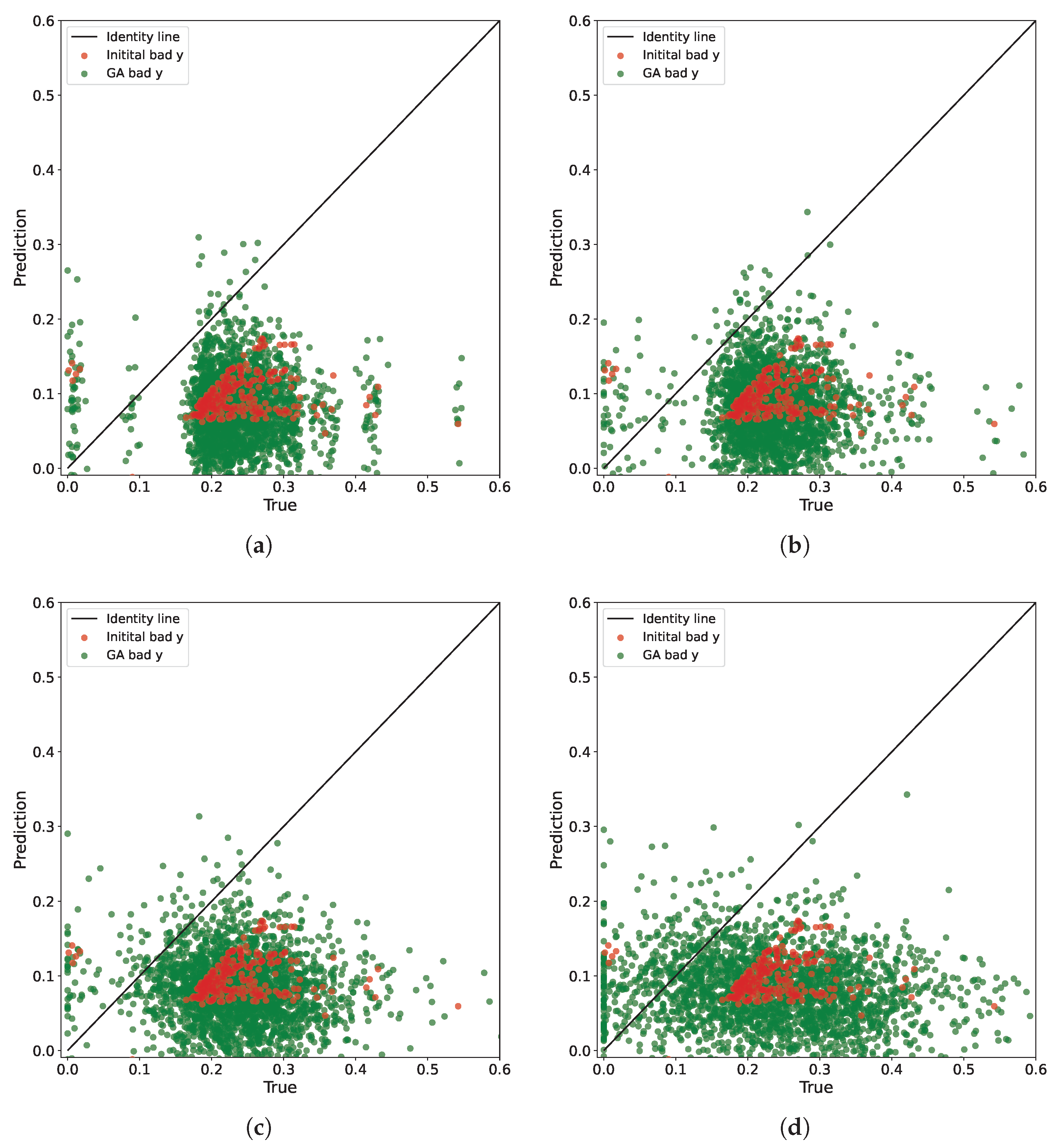
We identify the undesirable points using the threshold $\alpha =0.1$. Subsequently, we augment these points using our genetic algorithm. Figure 4 illustrates the prediction outcomes of the baseline model for various augmentations depending on the level of perturbation. Specifically, we select normal random variables with variances ${\sigma }_{\xi }^2$ of $0.005$, $0.02$, $0.05$, and $0.1$.

As is evident, selecting different levels of perturbations enables creating various augmentations and examining their impact on the prediction characteristics of the model. We only constrain the perturbation result within the range of the minimum and maximum values of $y_{te}$.

Table 1. Quantitative results for different augmentations levels.

Data	MSE	Wasserstein Distance for Target	Wasserstein Distance for Features	Residual Variance
Initial bad data	0.029	0.153	0.00	0.006
Augmented data with ${\sigma }_{\xi }^2=0.005$	0.039	0.171	0.090	0.010
Augmented data with ${\sigma }_{\xi }^2=0.02$	0.039	0.171	0.089	0.009
Augmented data with ${\sigma }_{\xi }^2=0.05$	0.041	0.170	0.092	0.012
Augmented data with ${\sigma }_{\xi }^2=0.1$	0.049	0.171	0.09	0.020

presents the quantitative outcomes for varying perturbation levels. It is observed that as the perturbation level increases, both the residual variance and the mean squared error of the predictions also increase. Despite this, the data similarity remains relatively close.

Figure 5 presents histograms illustrating the distributions of the test sample for the cases ${\sigma }_{\xi }^2=0.02$ and ${\sigma }_{\xi }^2=0.1$. While the histograms are normalized, this may slightly distort the visualization. Notably, the test sample contains bad points, but the majority of the data points are concentrated between $y_{min}$ and $0.3$. The regression model exhibits poor performance in the range from $0.3$ to $y_{max}$. Green represents the distribution of new points generated by the genetic algorithm. Considering that the initial bad points were perturbed by a random value with ${\sigma }_{\xi }^2=0.1$, it is evident that the augmented points are distributed beyond the main peak of the bad points, thereby encompassing their broader range.

Table A2. Comparison of prediction model results for regression problems on real-world dataset. We repeat the train–test split procedure 31 times and execute the entire pipeline on these distinct splits. For statistical significance, we provide the standard deviation.

Model	Threshold for Bad Points ($\mathit{\alpha }$)	Data	MSE (MEAN ± STD)	SMAPE (MEAN ± STD)	Wasserstein Ditance (MEAN ± STD)
Baseline model	$0.05$	$X_b$	$0.0070\pm 0.0003$	$0.6852\pm 0.0187$	—
		$X_{ga}$	$0.0144\pm 0.001$	$0.9737\pm 0.0099$	—
		$\tilde{X}$	$0.0136\pm 0.0010$	$0.9189\pm 0.0120$	$0.0229\pm 0.001$
	$0.1$	$X_b$	$0.0275\pm 0.0022$	$0.8933\pm 0.0175$	—
		$X_{ga}$	$0.0369\pm 0.0034$	$1.0903\pm 0.0294$	—
		$\tilde{X}$	$0.0360\pm 0.0034$	$1.0779\pm 0.0299$	$0.0278\pm 0.0017$
	$0.3$	$X_b$	$0.2228\pm 0.0602$	$1.4576\pm 0.0664$	—
		$X_{ga}$	$0.2612\pm 0.0859$	$1.6579\pm 0.1154$	—
		$\tilde{X}$	$0.2598\pm 0.0853$	$1.6674\pm 0.1275$	$0.0882\pm 0.0550$
Model for comparison	$0.05$	$X_b$	$0.0016\pm 0.0002$	$0.2012\pm 0.0105$	—
		$X_{ga}$	$0.0080\pm 0.0006$	$0.4867\pm 0.0099$	—
		$\tilde{X}$	$0.0064\pm 0.0004$	$0.4850\pm 0.0137$	$0.0229\pm 0.0010$
	$0.1$	$X_b$	$0.0083\pm 0.0018$	$0.2570\pm 0.0153$	—
		$X_{ga}$	$0.0168\pm 0.0021$	$0.5169\pm 0.0270$	—
		$\tilde{X}$	$0.0125\pm 0.0020$	$0.3974\pm 0.0392$	$0.0278\pm 0.0017$
	$0.3$	$X_b$	$0.1687\pm 0.0565$	$1.1056\pm 0.2443$	—
		$X_{ga}$	$0.1883\pm 0.0553$	$1.2383\pm 0.1758$	—
		$\tilde{X}$	$0.1922\pm 0.0561$	$1.2709\pm 0.1967$	$0.0882\pm 0.0550$

shows the quantitative results for the tabular data. For the baseline model, we employ linear regression, while gradient boosting serves as the model of comparison. We conduct three distinct experiments, each varying the threshold $\alpha$. The value $\alpha =0.05$ corresponds to $4\%$ of the bad points in $X_{te}$, and $\alpha =0.3$ corresponds to $0.02\%$. In these experiments, we evaluate the benchmark’s capability to function effectively with a limited number of bad points.

As is evident, the Wasserstein distance increases as the number of points decreases. This statistically significant effect may be attributed to the fact that the generator learns the distribution of bad points with lower accuracy when the number of instances is extremely low.

The MSE and SMAPE metrics also indicate that as the alpha value increases, the model quality deteriorates. This implies that as the bad points deviate more significantly from the overall distribution in the training sample, the model’s predictions for these points become less accurate.

The prediction results of the baseline model for different thresholds are illustrated in Figure 6.

5.5. Results for the Classification Model on Real-World Data

In this study, we employ the random forest classifier as the baseline model and the XGBoost classifier as the new tested model. Both models use a maximum depth of 3 and a total of 200 trees.

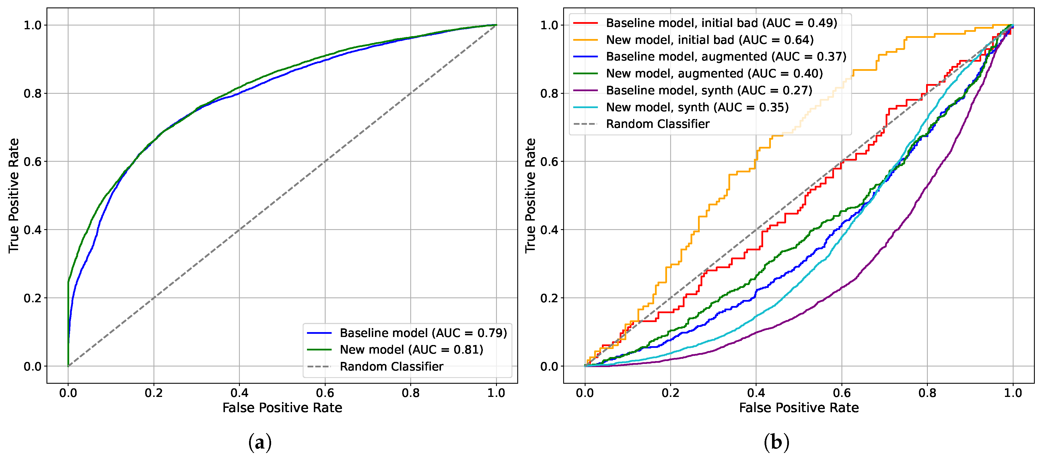
Figure 7 shows the Receiver Operating Characteristic (ROC) curve for the baseline and comparison models. It can be seen on the test data that the models behave very similarly to each other (Figure 7a). Nevertheless, the tested model surpasses the baseline in terms of quality. To further validate the new model, we emphasize the bad data points. Figure 7b presents the performance of the models on the challenging data points (orange and red lines). Notably, the tested model outperforms the baseline in terms of quality. The baseline exhibits behavior as a random classifier (gray dashed line).

Following the augmentation process, the new model exhibits behavior close to a random classifier, whereas the baseline model behaves as an inverse classifier. In essence, if we invert the predictions of the baseline model, it demonstrates improved performance. The same patterns can be seen for the synthetic dataset (cyan and purple lines).

The quantitative results are presented in

Table A3. Comparison of the prediction model results for classification problems on real-world datasets. We repeat the train–test split procedure 31 times and execute the entire pipeline on these distinct splits. For statistical significance, we provide the standard deviation.

Model	Threshold for Bad Points ($\mathit{\alpha }$)	Data	${\mathit{F}}_1$ (MEAN ± STD)	ROCAUC (MEAN ± STD)	Wasserstein Distance (MEAN ± STD)
Baseline model	$0.501$	$X_b$	$0.4537\pm 0.0654$	$0.5068\pm 0.0495$	—
		$X_{ga}$	$0.4506\pm 0.0639$	$0.5031\pm 0.0451$	—
		$\tilde{X}$	$0.3623\pm 0.0735$	$0.4901\pm 0.0579$	$0.0487\pm 0.0106$
	$0.502$	$X_b$	$0.4808\pm 0.0536$	$0.5119\pm 0.0404$	—
		$X_{ga}$	$0.4838\pm 0.0498$	$0.5113\pm 0.0395$	—
		$\tilde{X}$	$0.3736\pm 0.0828$	$0.4901\pm 0.0510$	$0.0496\pm 0.0067$
	$0.505$	$X_b$	$0.4670\pm 0.0367$	$0.5081\pm 0.0248$	—
		$X_{ga}$	$0.4720\pm 0.0359$	$0.5092\pm 0.0241$	—
		$\tilde{X}$	$0.3954\pm 0.1078$	$0.4968\pm 0.0402$	$0.0380\pm 0.0047$
Model for comparison	$0.501$	$X_b$	$0.4334\pm 0.0876$	$0.5546\pm 0.0602$	—
		$X_{ga}$	$0.4181\pm 0.0853$	$0.5478\pm 0.0574$	—
		$\tilde{X}$	$0.2189\pm 0.1019$	$0.5383\pm 0.0375$	$0.0487\pm 0.0106$
	$0.502$	$X_b$	$0.4457\pm 0.0684$	$0.5548\pm 0.0355$	—
		$X_{ga}$	$0.4271\pm 0.0695$	$0.5483\pm 0.0354$	—
		$\tilde{X}$	$0.2115\pm 0.0937$	$0.5307\pm 0.0361$	$0.0496\pm 0.0067$
	$0.505$	$X_b$	$0.4241\pm 0.0636$	$0.5522\pm 0.0244$	—
		$X_{ga}$	$0.3965\pm 0.0647$	$0.5438\pm 0.0228$	—
		$\tilde{X}$	$0.1168\pm 0.0867$	$0.5222\pm 0.0244$	$0.0380\pm 0.0047$

. It is noteworthy that the newly tested model does not exhibit superior performance compared to the baseline model in terms of the ROCAUC metrics. However, it demonstrates statistically significant improvement in terms of the $F_1$ metrics.

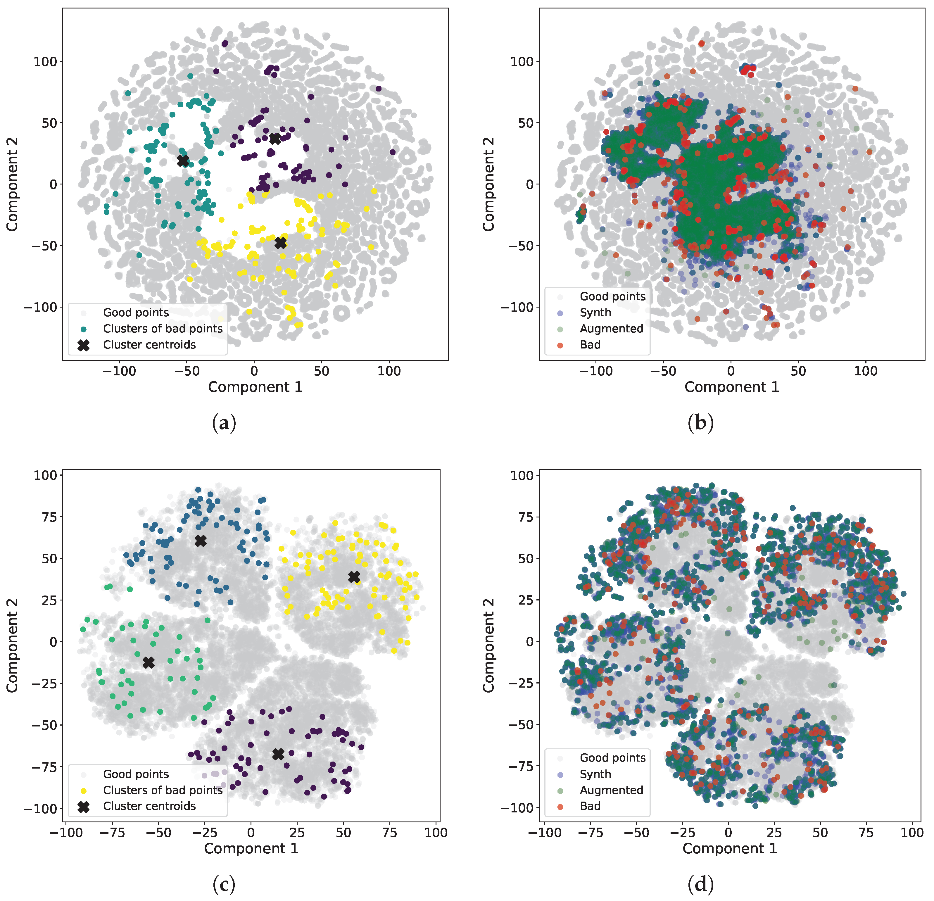
Figure 8 illustrates the qualitative results of synthetic data generation for both regression and classification tasks. For regression problems, we use t-distributed stochastic neighbor embeddings (t-SNE) algorithm with a perplexity of 15, a random state of 42, and PCA initialization. We apply the t-SNE algorithm to the dataset, which comprises initial bad points from the test set, good points from the test set, augmented points (generated after applying the genetic algorithm), and synthetic points (generated after applying the VAE model). We also apply the K-means clustering algorithm to identify clusters of bad points. The number of clusters is determined empirically and equals three.

It is noteworthy that the most significant bad points are predominantly located near the boundary of an empty area. While some points are located away from the boundary, this may be attributed to the dimension reduction process (Figure 8a). In Figure 8b, it is evident that the points generated after augmentation using the genetic algorithm completely encompass the empty area. The points generated by the VAE model cover the same area but exhibit a denser distribution. Therefore, it can be inferred that the newly identified bad points are not random fluctuations but rather exhibit a systematic pattern.

For classification problems, we employ t-SNE with a perplexity of 30, a random state of 42, and PCA initialization. Additionally, we use the K-means clustering algorithm with four clusters. These four clusters are distinctly visible in Figure 8c and encompass various regions of space. Unlike regression, there is no clearly defined area of poor points, as the task itself is more challenging due to the binary target. However, we can still observe the performance of the genetic algorithm and generative model, which effectively describe the boundaries of the areas. In other words, by generating synthetic points, we can understand the concentration of a significant number of bad points. Furthermore, in both regression and classification scenarios, synthetic data clearly encompass the original bad data.

5.6. Hyperparameters

The VAE model is trained using the AdamW optimizer [27] with an initial learning rate of $1\times {10}^{-3}$ and a cosine scheduler that decreases the learning rate to $1\times {10}^{-4}$. During training, the gradient norm is clipped to a maximum value of three. To enhance convergence, a scheduler is also used for the KL divergence coefficient within the loss function. Initially set at $0.0$, the KL divergence coefficient is uniformly increased over half of the epochs, reaching a maximum of $5\times {10}^{-4}$. Subsequently, it is incrementally increased from $5\times {10}^{-4}$ to $1\times {10}^{-2}$ for the remaining epochs.

In experiments involving a substantial number of bad points, we employ varying batch sizes. For instance, when $\alpha =0.05$, we use a batch size of 256 for real-world data. For $\alpha =0.3$, we use a batch size of 16.

Table 2. Full list of hyperparameters in our benchmark model for both toy and real-world datasets.

Hyperparameter	Toy example	Regression	Classification
Number of features	2	16	12
Number of categorical features	0	1	4
The threshold $\alpha$	$0.1$	$0.05, 0.1, 0.3$	$0.501, 0.502, 0.505$
Number of steps in GA	20	$5, 10, 20$	$8, 5, 3$
Batch size	16	$256, 128, 16$	$64, 128, 256$
Number of epochs	100	$200, 200, 100$	$100, 100, 200$
Optimizer	AdamW	AdamW	AdamW
Initial learning rate	$1\times {10}^{-3}$	$1\times {10}^{-3}$	$1\times {10}^{-3}$
Gradient max norm clip	3	3	3
Scheduler	CosineAnnealingLR	CosineAnnealingLR	CosineAnnealingLR
Minimum learning rate	$1\times {10}^{-4}$	$1\times {10}^{-4}$	$1\times {10}^{-4}$
Cross-entropy loss multiplier	$0.1$	$0.1$	$0.1$
Hidden channels	16	16	16
Latent dimension	64	256	256
Categorical embedding latent dimension	0	4	4
Decoder hidden dimension	32	512	512
Activation function	SiLU	SiLU	SiLU

presents a comprehensive list of hyperparameters, including the number of features, the genetic algorithm configuration, and the variational autoencoder configuration.

6. Discussion

Our approach can also be adapted to multi-output regression. For multi-output regression, we can select problematic points in the same manner by comparing the residual with a threshold value $\alpha$ and averaging across all output targets. Alternatively, we can select problematic points for each target individually and then choose the intersection or union of these points. We must also modify the generator by altering the condition in the encoder and decoder. Instead of a single value, it will now be a vector.

Another application of the proposed approach is its use with time series prediction models. To create a dataset of the form $\{X,y\}$, we can divide the time series into windows and select the target value as the next value within the window. This approach allows for the use of the same genetic operators and, for generative models, the selection of task-specific generators [28,29,30].

Our pipeline presents a potential application for assessing the quality of large language models (LLMs). Currently, there is a pressing need to evaluate the quality of LLMs. Existing benchmark datasets often show that increasingly advanced models consistently achieve high results. However, rather than creating fundamentally new benchmark datasets, it is possible to study the quality of models based on previous ones. Our method can be adapted for this purpose.

Specifically, it is feasible to augment complex tasks in current benchmark datasets to increase the number of examples, resulting in a significant improvement in effectiveness. However, compared to classical tabular data, augmenting text tasks requires defining the rules of mutation and crossover operators for the genetic algorithm. Once such rules are defined, we immediately gain the opportunity to balance between the similarity of tasks within the current benchmark and tasks that are fundamentally different, potentially at the boundary of the defined domain.

It may be interesting to extend our approach in other contexts, such as considering a multi-agent system with diverse regression models. During agent interaction, it is crucial to identify the most suitable models to retain or discard. This can be achieved by conducting a series of experiments using automatic benchmark dataset generation to assess model performance.

7. Conclusions

In this paper, we demonstrated a mechanism for constructing automatic benchmark datasets for data-driven models in classical machine learning based on their errors. We analyzed the case of regression, where the target is a continuous feature, and the case of classification problems for a binary target.

Using our methodology, researchers can construct adaptive benchmark datasets to assess the performance of their models. Future enhancements could involve exploring alternative approaches to introduce perturbations in the initial distribution of bad data points, thereby improving or replacing the genetic algorithm with a more suitable method. Furthermore, advancements in distribution estimation techniques are also feasible. For instance, utilizing diffusion models or other models capable of effectively approximating the structure of tabular data as a generative model could be beneficial.

References

1. Feng, Y.; Long, Y.; Wang, H.; Ouyang, Y.; Li, Q.; Wu, M.; Zheng, J. Benchmarking machine learning methods for synthetic lethality prediction in cancer. Nat. Commun. 2024, 15, 9058. [Google Scholar] [CrossRef]
2. Maheshwari, G.; Ivanov, D.; Haddad, K.E. Efficacy of synthetic data as a benchmark. arXiv 2024, arXiv:2409.11968. [Google Scholar] [CrossRef]
3. Liu, Y.; Khandagale, S.; White, C.; Neiswanger, W. Synthetic benchmarks for scientific research in explainable machine learning. arXiv 2021, arXiv:2106.12543. [Google Scholar] [CrossRef]
4. Nikitin, N.O.; Vychuzhanin, P.; Sarafanov, M.; Polonskaia, I.S.; Revin, I.; Barabanova, I.V.; Maximov, G.; Kalyuzhnaya, A.V.; Boukhanovsky, A. Automated evolutionary approach for the design of composite machine learning pipelines. Future Gener. Comput. Syst. 2022, 127, 109–125. [Google Scholar] [CrossRef]
5. He, X.; Zhao, K.; Chu, X. AutoML: A survey of the state-of-the-art. Knowl.-Based Syst. 2021, 212, 106622. [Google Scholar] [CrossRef]
6. Truong, A.; Walters, A.; Goodsitt, J.; Hines, K.; Bruss, C.B.; Farivar, R. Towards automated machine learning: Evaluation and comparison of AutoML approaches and tools. In Proceedings of the 2019 IEEE 31st International Conference on Tools with Artificial Intelligence (ICTAI), Portland, OR, USA, 4–6 November 2019; IEEE: Piscataway, NJ, USA, 2019; pp. 1471–1479. [Google Scholar]
7. Longjohn, R.; Kelly, M.; Singh, S.; Smyth, P. Benchmark data repositories for better benchmarking. Adv. Neural Inf. Process. Syst. 2024, 37, 86435–86457. [Google Scholar]
8. Demetriou, D.; Mavromatidis, P.; Petrou, M.F.; Nicolaides, D. CODD: A benchmark dataset for the automated sorting of construction and demolition waste. Waste Manag. 2024, 178, 35–45. [Google Scholar] [CrossRef]
9. Xia, C.S.; Deng, Y.; Zhang, L. Top Leaderboard Ranking = Top Coding Proficiency, Always? EvoEval: Evolving Coding Benchmarks via LLM. arXiv 2024, arXiv:2403.19114. [Google Scholar] [CrossRef]
10. Mahdavi, H.; Hashemi, A.; Daliri, M.; Mohammadipour, P.; Farhadi, A.; Malek, S.; Yazdanifard, Y.; Khasahmadi, A.; Honavar, V. Brains vs. bytes: Evaluating llm proficiency in olympiad mathematics. arXiv 2025, arXiv:2504.01995. [Google Scholar] [CrossRef]
11. Shi, Q.; Tang, M.; Narasimhan, K.; Yao, S. Can Language Models Solve Olympiad Programming? arXiv 2024, arXiv:2404.10952. [Google Scholar] [CrossRef]
12. Zheng, Z.; Cheng, Z.; Shen, Z.; Zhou, S.; Liu, K.; He, H.; Li, D.; Wei, S.; Hao, H.; Yao, J.; et al. LiveCodeBench Pro: How Do Olympiad Medalists Judge LLMs in Competitive Programming? arXiv 2025, arXiv:2506.11928. [Google Scholar]
13. Ang, Y.; Huang, Q.; Bao, Y.; Tung, A.K.H.; Huang, Z. TSGBench: Time Series Generation Benchmark. arXiv 2023, arXiv:2309.03755. [Google Scholar] [CrossRef]
14. Yao, B.M.; Wang, Q.; Huang, L. Error-driven Data-efficient Large Multimodal Model Tuning. In Proceedings of the 63rd Annual Meeting of the Association for Computational Linguistics (Volume 1: Long Papers); Association for Computational Linguistics: Vienna, Austria, 2025; pp. 20289–20306. [Google Scholar]
15. Mendes, P.; Romano, P.; Garlan, D. Error-driven uncertainty aware training. arXiv 2024, arXiv:2405.01205. [Google Scholar] [CrossRef]
16. Chandra, A.; Yao, X. Ensemble Learning Using Multi-Objective Evolutionary Algorithms. J. Math. Model. Algorithms 2006, 5, 417–445. [Google Scholar] [CrossRef]
17. Brown, G.; Wyatt, J.; Harris, R.; Yao, X. Diversity creation methods: A survey and categorisation. Inf. Fusion 2005, 6, 5–20. [Google Scholar] [CrossRef]
18. Abdollahi, J.; Nouri-Moghaddam, B. Hybrid stacked ensemble combined with genetic algorithms for diabetes prediction. Iran J. Comput. Sci. 2022, 5, 205–220. [Google Scholar] [CrossRef]
19. Shojaee, P.; Nguyen, N.H.; Meidani, K.; Farimani, A.B.; Doan, K.D.; Reddy, C.K. LLM-SRBench: A New Benchmark for Scientific Equation Discovery with Large Language Models. arXiv 2025, arXiv:2504.10415. [Google Scholar] [CrossRef]
20. Rafiei Oskooei, A.; Babacan, M.; Yağci, E.; Alptekin, C.; Buğday, A. Beyond Synthetic Benchmarks: Assessing Recent LLMs for Code Generation. In Proceedings of the 14th International Workshop on Computer Science and Engineering (WCSE 2024), Phuket Island, Thailand, 19–21 June 2024. [Google Scholar] [CrossRef]
21. Ronchetti, E.M.; Huber, P.J. Robust Statistics; John Wiley & Sons: Hoboken, NJ, USA, 2009. [Google Scholar]
22. Pedregosa, F.; Varoquaux, G.; Gramfort, A.; Michel, V.; Thirion, B.; Grisel, O.; Blondel, M.; Prettenhofer, P.; Weiss, R.; Dubourg, V.; et al. Scikit-learn: Machine Learning in Python. J. Mach. Learn. Res. 2011, 12, 2825–2830. [Google Scholar]
23. Syswerda, G. Uniform crossover in genetic algorithms. In Proceedings of the Third International Conference on Genetic Algorithms and Their Application, Morgan Kaufmann, San Mateo, CA, USA, 1 December 1989; pp. 2–9. [Google Scholar]
24. Blickle, T. Tournament selection. Evol. Comput. 2000, 1, 188. [Google Scholar]
25. Fortin, F.A.; De Rainville, F.M.; Gardner, M.A.; Parizeau, M.; Gagné, C. DEAP: Evolutionary Algorithms Made Easy. J. Mach. Learn. Res. 2012, 13, 2171–2175. [Google Scholar]
26. Perez, E.; Strub, F.; De Vries, H.; Dumoulin, V.; Courville, A. Film: Visual reasoning with a general conditioning layer. In Proceedings of the AAAI Conference on Artificial Intelligence, New Orleans, LA, USA, 2–7 February 2018; Volume 32. [Google Scholar]
27. Loshchilov, I.; Hutter, F. Decoupled weight decay regularization. arXiv 2017, arXiv:1711.05101. [Google Scholar]
28. Zakharov, K.; Stavinova, E.; Boukhanovsky, A. Synthetic financial time series generation with regime clustering. J. Adv. Inf. Technol 2023, 14, 1372–1381. [Google Scholar] [CrossRef]
29. Yuan, X.; Qiao, Y. Diffusion-ts: Interpretable diffusion for general time series generation. arXiv 2024, arXiv:2403.01742. [Google Scholar] [CrossRef]
30. Liao, S.; Ni, H.; Szpruch, L.; Wiese, M.; Sabate-Vidales, M.; Xiao, B. Conditional sig-wasserstein gans for time series generation. arXiv 2020, arXiv:2006.05421. [Google Scholar] [CrossRef]
Figure 1. Benchmark pipeline. The dataset D is divided into training and test sets. Transformations are then trained on the training set, and the test set is transformed based on these transformations. Then, the model F is trained and applied to the test set. The operator K is applied to the predicted values, and the bad points are identified. Finally, augmentation and generation of new bad data points are performed.
Make 07 00148 g001
Figure 2. Variational autoencoder pipeline. The encoder and decoder architectures process features with several convolutional and linear layers and use the targets for linear modulation as the conditions. Data tensors are visually represented in teal. Linear projections, non-linear activation functions, and convolution operations are depicted in blue, while block representations of layer combinations such as convolutions, activation functions, and normalizations are shown in red boxes. The symbol × denotes element-wise multiplication, and + denotes element-wise summation. The embedding layer for categorical features is distinguished by a light green and consists of a set of matrices for each category. These matrices are trainable and have dimensions with rows corresponding to the number of unique categories in a categorical feature and columns corresponding to the fixed embedding size. Solid arrows represent the primary data processing, while dashed lines indicate optional processing for categorical data.
Make 07 00148 g002
Figure 3. (a) The synthetic dataset. (b) The bad examples were after the baseline regression model was trained. (c) New augmented points after the genetic algorithm was applied. (d) The prediction results on the bad points and GA points. (e) The points generated by the VAE model. (f) The prediction results for the baseline and the new model for comparison on the synthetic dataset.
Make 07 00148 g003
Figure 4. The prediction results on the bad points (Initial bad) and augmented points (GA bad) with the genetic algorithm for the different perturbation levels. The optimal prediction results align with the identity line. The graphs illustrate that as the perturbation level in the genetic algorithm increases, the model’s predictions become more diverse and encompass previously unexplored regions where the model exhibits poor performance. It is noteworthy that due to the inherent randomness of the algorithm and the fixed number of steps, we encounter instances where the model exhibits satisfactory predictions. However, these favorable points are removed by repeated application of the operator K. (a) σ 2 = 0.005 . (b) σ 2 = 0.02 . (c) σ 2 = 0.05 . (d) σ 2 = 0.1 .
Make 07 00148 g004
Figure 5. Histograms of the distributions for test set (blue), bad (red), and augmented (green) points for different perturbation levels σ 2 . The X-axis represents the normalized target values, while the Y-axis represents the normalized frequencies. (a) σ 2 = 0.02 . (b) σ 2 = 0.1 . Graph (b) illustrates the progressive coverage of target values by augmented points as the perturbation level increases.
Make 07 00148 g005
Figure 6. Prediction outcomes of the baseline model for various thresholds on the test set for real-world regression data. The optimal prediction results align with the identity line. Points identified as bad are highlighted in red, while points from the test dataset are highlighted in blue. (a) α = 0.05 . (b) α = 0.1 . (c) α = 0.3 .
Make 07 00148 g006
Figure 7. Receiver operating characteristic (ROC) curve. The X-axis represents the false positive rate, which is the proportion of instances where the model incorrectly predicts a label of «1» when the actual label is «0». The Y-axis represents the true positive rate, which is the proportion of actual labels of «1» that are correctly identified by the model. (a) ROC curve for the test sample. (b) ROC curve for the bad, augmented, and synthetic points.
Make 07 00148 g007
Figure 8. Visualization of t-distributed stochastic neighbor embeddings (t-SNE) components. Gray points represent good data, red points represent bad data, green points represent augmented data, and blue points correspond to synthetic data. (a) t-SNE components for regression problems with clusters of bad points. Clusters are visually distinguished by three distinct colors. (b) t-SNE components for regression problems with bad, augmented, and synthetic points. (c) t-SNE components for classification problems with clusters of bad points. Clusters are visually distinguished by four distinct colors. (d) t-SNE components for classification problems with bad, augmented, and synthetic points.
Make 07 00148 g008