A Graph-Structured, Physics-Informed DeepONet Neural Network for Complex Structural Analysis

Abstract

This study introduces the Graph-Structured Physics-Informed DeepONet (GS-PI-DeepONet), a novel neural network framework designed to address the challenges of solving parametric Partial Differential Equations (PDEs) in structural analysis, particularly for problems with complex geometries and dynamic boundary conditions. By integrating Graph Neural Networks (GNNs), Deep Operator Networks (DeepONets), and Physics-Informed Neural Networks (PINNs), the proposed method employs graph-structured representations to model unstructured Finite Element (FE) meshes. In this framework, nodes encode physical quantities such as displacements and loads, while edges represent geometric or topological relationships. The framework embeds PDE constraints as soft penalties within the loss function, ensuring adherence to physical laws while reducing reliance on large datasets. Extensive experiments have demonstrated the GS-PI-DeepONet’s superiority over traditional Finite Element Methods (FEMs) and standard DeepONets. For benchmark problems, including cantilever beam bending and Hertz contact, the model achieves high accuracy. In practical applications, such as stiffness analysis of a recliner mechanism and strength analysis of a support bracket, the framework achieves a 7–8 speed-up compared to FEMs, while maintaining fidelity comparable to FEM, with R² values reaching up to 0.9999 for displacement fields. Consequently, the GS-PI-DeepONet offers a resolution-independent, data-efficient, and physics-consistent approach for real-time simulations, making it ideal for rapid parameter sweeps and design optimizations in engineering applications.

1. Introduction

Recent years have witnessed remarkable breakthroughs in solving Partial Differential Equations (PDEs) using deep learning [1]. In 2018, Raissi, Perdikaris, and Karniadakis introduced Physics-Informed Neural Networks (PINNs) [2], a framework that incorporates physical laws as soft constraints within the loss function, delivering continuous, strong-form solutions. Since then, PINNs have been successfully applied to heat transfer [3,4], solid mechanics [5,6], and fluid mechanics [7], bridging classical numerical solvers with modern deep learning.

Recent advances in PINNs have focused on improving their computational efficiency and numerical stability for high-order PDE systems. He et al. pioneered multi-level PINNs that decompose the solution process across multiple scales, demonstrating a four-fold acceleration over conventional PINNs while preserving FE accuracy [8]. This approach was further refined through adaptive hierarchical sampling, achieving additional 30% speed improvements for stiffness analysis problems [9]. The community has subsequently developed several innovative variants to address fundamental limitations: weak-form formulations that mitigate gradient pathologies through variational principles [10,11,12]; distributed architectures that enhance scalability via domain decomposition [13,14]; and stabilized versions that incorporate numerical dissipation mechanisms for advection-dominated flows [14]. While these developments show theoretical promise, comprehensive benchmarking studies reveal that PINNs’ practical advantages over traditional solvers remain problem-dependent [15], with current successful deployments primarily concentrated in inverse problems [16], parameter estimation tasks [17,18,19,20,21].

Concurrently, spatial-feature extraction models based on convolutional or Graph Neural Networks (GNNs) have emerged for discrete PDE solutions [22]. In 2019, Lu et al. proposed Deep Operator Networks (DeepONets) [23], which extend surrogate modeling from finite-dimensional functions to general nonlinear operators acting on infinite-dimensional spaces. By leveraging the universal approximation theorem for operators, DeepONets allow for resolution-independent, continuous output representations and can be trained with minimal data when physical constraints are embedded in the loss function. Recently, Key developments have focused on enhancing architectural expressivity and efficiency through novel designs like Transformer-based architectures [24] and Factorized Fourier Neural Operators (F-FNO) [25], which better capture long-range dependencies and offer spectral convergence. The integration of physics-informed learning has been deepened, with a growing emphasis on handling multi-physics problems through auxiliary parameter inputs [26] and on improving training stability using weak formulations and variational losses to circumvent high-order derivatives. A major research thrust has been improving scalability and generalization, addressed through meta-learning for few-shot operator learning and advanced transfer learning techniques. Furthermore, the application scope of DeepONets has dramatically expanded to tackle more complex real-world challenges, including the modeling of stochastic partial differential equations (SPDEs) [20,27,28] and long-time, multi-scale turbulent flows [29,30]. Diab et al. later introduced DeepOKAN, a variant of the Kolmogorov–Arnold network that improves accuracy and efficiency for multi-physics problems in additive manufacturing [31]. Very recently, research has begun to focus on enhancing the foundational robustness and theoretical understanding of these models. This includes work on bounding generalization errors for operator learning frameworks, developing more sample-efficient training strategies, and creating unified frameworks that seamlessly integrate various neural operator architectures like DeepONet and FNO for broader applicability and improved performance on industrial-scale problems.

Another important issue is graph-based simulators. Sanchez-Gonzalez et al. proposed the Graph Network Simulator (GNS) to predict particle dynamics in real time [32]; Pfaff et al. extended this idea to MeshGraphNets for learning mesh-based simulations in structural mechanics, aerodynamics, and cloth dynamics [33]. A pivotal advancement has been the widespread adoption of geometric equivariance, with E(n)-equivariant GNNs ensuring predictions remain consistent under translations, rotations, and reflections, thereby enhancing physical correctness and data efficiency [34,35,36]. Building on foundational mesh-based learning frameworks [33], research has significantly improved the handling of complex and dynamic geometries, enabling the simulation of problems on unstructured meshes and deforming domains [37]. Furthermore, the field has moved towards building robust and generalizable surrogates, with GNNs being applied to multi-scale continuum mechanics [38] and inverse problems [39], culminating in efforts to create universal physical simulators that generalize across diverse conditions [40]. While promising, these methods still suffer from message-passing bottlenecks on high-resolution meshes, limiting their scalability. Physics-Guided Neural Networks (PGNNs) [41] and Physics-encoded Neural Networks (PeNNs) offer additional avenues for embedding physical priors [42].

Generally, deep learning methods have demonstrated significant potential in structural mechanics simulation and analysis, particularly in addressing the issues of high computational costs and low efficiency associated with traditional numerical methods. However, their application still faces challenges in terms of generalizability, real-time performance, and handling complex models. Therefore, constructing an efficient, real-time intelligent simulation solver that integrates data-driven approaches, deep learning, traditional numerical methods, and large-scale computing has become a major research focus in structural analysis.

Therefore, an alternative hybrid framework that unifies the strengths of GNNs, DeepONets, and PINNs into a single architecture—the Graph-Structured Physics-Informed DeepONet (GS-PI-DeepONet) is suggested. The framework leverages graph representations to handle unstructured meshes and complex geometries, while embedding PDE constraints to ensure physical consistency. By combining operator learning with physics-informed regularization, GS-PI-DeepONet achieves better accuracy, efficiency, and generalization compared to the vanilla DeepONet, as demonstrated in both benchmark problems and real-world engineering applications. The proposed approach not only addresses the data hunger and resolution dependence of traditional DeepONets but also provides a scalable solution for real-time structural analysis under varying boundary conditions and geometric configurations.

Therefore, a hybrid framework that integrates the strengths of Graph Neural Networks (GNNs), DeepONets, and Physics-Informed Neural Networks (PINNs) into a unified architecture—termed the Graph-Structured Physics-Informed DeepONet (GS-PI-DeepONet) is proposed.

Generally, this study introduces two key innovations in operator learning for engineering applications. First, it proposes a holistic graph-structured representation for handling unstructured Finite Element meshes and complex geometries, where nodes encode physical quantities and edges represent geometric connectivity, eliminating the need for structured grids or data interpolation. Second, it develops a physics-informed, data-efficient framework that uniquely integrates PINNs as a regularizer within the graph-based DeepONet training. This hybrid co-optimization allows the model to learn from both limited simulation data and governing physical laws simultaneously. As validated through benchmark problems and real-world engineering applications. The proposed approach not only alleviates the data dependency and resolution constraints of traditional DeepONets but also provides a scalable solution for real-time structural analysis across various boundary conditions and geometric configurations.

2. Motivations

The primary purpose of structural analysis is to obtain, for a deformable body of arbitrary geometric complexity, the complete and accurate information about mechanical changes—namely displacement, strain, and stress—induced within the body by intricate external loads. Mathematically, this task is formulated as the solution to a parametric PDE problem, with governing equations expressed as conservation laws and constitutive relations in differential form as

$$\mathcal{N}\left(u;\mu \right)=0 \mathrm{i}\mathrm{n} \Omega \left(\mu \right),\mathcal{B}\left(u;\mu \right)=0 \mathrm{o}\mathrm{n} \mathit{\partial }\Omega \left(\mu \right),$$

(1)

where $\mu$ denotes a parameter vector encompassing material properties, geometric descriptors, initial/boundary conditions, or any other scenario-defining quantities; $\Omega \left(\mu \right)\subset {\mathbb{R}}^{\mathrm{d}}$ is the parameter-dependent spatial domain; $u$ is the unknown PDE solution (e.g., displacement field); $\mathcal{N}$ and $\mathcal{B}$ are (possibly nonlinear) differential and boundary operators, respectively.

Generally, for a parametric PDE problem, the parameter-to-solution map defines an operator

$$\mathcal{G}:\mu \mapsto u(\cdot ;\mu ),$$

(2)

which we seek to approximate efficiently.

Traditional numerical solvers, with FEMs as a prime example, necessitate a complete re-simulation for each new parameter instance, resulting in excessive computational costs. In recent years, neural-network tools have been actively developed to infer solutions to PDEs; however, most existing approaches are still limited to a fixed geometry and a given set of input parameters as well as initial and boundary conditions. Despite these limitations, neural networks continue to be a popular research topic and have found widespread application in science and engineering, already demonstrating good performance in high-dimensional problems.

To solve the aforementioned limitations, neural operator techniques express the solution map $\mathrm{G}$ as an integral Hilbert–Schmidt operator. The structural analysis problem is therefore recast as learning a discrete approximation of the operator that maps boundary/initial data to the solution function. Figure 1 illustrates this concept for a simple parameterized simply supported beam, modeled by the Banach-space triplet $(U,V,W)$ with the differential operator written compactly as

$${\mathcal{L}}_{\mu }:\mathcal{U}\to \mathcal{V},{\mathcal{L}}_{\mu }u=f.$$

(3)

Given input functions $a\left(\mu \right)$, the parametric PDE problem is

$${\mathcal{L}}_{\mu }\left(u\right)=f\left(\mu \right),u{|}_{\mathit{\partial }\Omega }=g\left(\mu \right),$$

(4)

and, under standard well-posed assumptions, the solution operator becomes

$$\mathcal{G}:a\left(\mu \right)\mapsto u(\cdot ;\mu ).$$

(5)

Neural operators allow querying the solution at arbitrary spatial locations. Lu et al., extending the universal-approximation theorem to operators, introduced DeepONets—an architecture that approximates any continuous operator by an inner product of latent encodings of input and output function spaces [23]. However, DeepONets rely on point-wise function values sampled on a fixed mesh. Consequently, the predicted solution is merely a finite-dimensional approximation that may contradict the underlying PDE, especially in highly nonlinear or rapidly varying fields. Moreover, the discrete representation inflates data requirements. Generating the requisite dataset often demands repeated high-fidelity finite-element analyses or costly experiments.

Graph-based deep operator networks present a promising solution. By utilizing GNNs, they adapt effortlessly to data with varying resolutions and capture the geometric complexities of finite-element meshes. GNNs, with their message-passing mechanisms, inherently manage non-Euclidean data such as meshes, point clouds, or molecular structures. In structural analysis, each node represents physical quantities (such as displacements, strains), while edges encode geometric connectivity or physical coupling, transforming the high-dimensional continuum into an explicit graph representation that is rich in geometric semantics. The creation of these graphs is guided by CAE (Computer-Aided Engineering)software Calculix 2.22 simulation results: once a post-processed field is available, nodal variables are systematically extracted along with their topological relationships, resulting in a structured graph.

Nonetheless, the explicit storage of large adjacency matrices and iterative message passing result in significant memory footprints. To mitigate this, PINNs are seamlessly integrated into the graph-learning framework. By embedding the strong-form PDE residual directly into the loss function and leveraging automatic differentiation to implicitly encode differential operators, the model is encouraged to produce outputs that satisfy the governing equations without ever materializing the high-dimensional stiffness matrix. This strategy alleviates memory bottlenecks and, more importantly, injects physical priors that enhance generalization and reduce the amount of observational data required—an advantage most pronounced in regimes of sparse training data or dynamically evolving geometries. For these reasons, a graph-structured, physics-informed deep operator network is suggested to satisfy the geometrical and physical requirements for the computation of PDEs.

3. Graph-Structured Physical-Informed DeepONet

The purpose of GS-PI-DeepONet neural framework is to tackle the difficulties associated with solving parametric PDEs in structural analysis, especially for issues that involve complex geometries and boundary conditions. This method combines GNNs with Physical-Informed Deep Operator Networks (PI-DeepONets), harnessing the advantages of both approaches to provide efficient, and accurate solutions. Compared to vanilla DeepONets, GS-PI-DeepONet surpasses this limitation by utilizing graph-structured representations. In this context, nodes encode physical quantities such as displacements and loads, while edges represent geometric or topological relationships. This allows the model to adapt seamlessly to unstructured meshes or point clouds, which are common in FE analysis. Moreover, to enhance the efficiency and accuracy of the solution, PINNs are introduced and PDEs are embedded as soft constraints—irrespective of input dimensionality. The details of GS-PI-DeepONet are presented as follows.

3.1. Geometric (Graph Attention Networks) Embedding DeepONet

In structural analysis, inputs such as material distribution and boundary conditions, as well as outputs like solutions, often exist in the form of unstructured grids, typically represented as FE mesh node data or 3D point cloud topologies. Traditional data-driven methods face significant limitations in such problems: fully connected networks ignore geometric topological information and forcibly fit input-output mappings through dense weight matrices, leading to an exponential expansion of the parameter space. This not only drastically increases computational resource consumption but also raises severe overfitting risks. Graph-structured data can share weights across different nodes, significantly reducing the number of parameters while effectively capturing complex geometric relationships. Through message-passing mechanisms, it can also model local strain and global stress transmission paths, enabling efficient feature extraction from the data.

A graph represents relationships between a set of entities—nodes and edges in finite element analysis—and can generally be expressed as $G=(V,E)$, where $V$ is the set of all vertices in the graph, and $E$ is the set of all edges. To further describe each node, edge, or the entire graph, information can be stored in various parts of the graph.

Let $v_i$ be a node in the graph, and $e_{ij}$ be an edge from node $v_i$ to node $v_j$. The neighborhood of node $v_i$ is $N\left(v_{\mathrm{i}}\right)$, which is the set of all nodes adjacent to $v_i$. For the adjacency matrix $\mathrm{A}$ of the graph, if $e_{ij}\in E$, then $A_{ij}=1$; otherwise, $A_{ij}=0$. The size of the matrix is $\left|V\right|\times \left|V\right|$.

Commonly used graph neural network models include Graph Convolutional Networks (GCNs), Graph Attention Networks (GATs), and Gated Graph Neural Networks (GGNNs). Among these, GCNs draw inspiration from CNNs (Convolutional Neural Networks) and aim to generalize traditional convolution operations to non-Euclidean spaces, i.e., graph-structured data. The core idea is the neighborhood aggregation mechanism, which updates node representations using the features of nodes and their neighbors, thereby capturing local and global graph features. Unlike CNNs, which extract features from local neighborhoods on regular grids (e.g., image data), GCNs aggregate information from neighboring nodes to update the current node’s representation, capturing local dependencies in the graph structure.

Generally, graph-structured data can be described using the Laplacian matrix:

$$L=D-A$$

(6)

where $A$ is the adjacency matrix, representing connections between nodes, $D$ is the degree matrix, with diagonal elements indicating the number of neighbors for each node.

For numerical stability, the normalized Laplacian matrix is often used

$$L_{\mathrm{norm}}=I-D^{-1/2}A{D}^{-1/2}$$

(7)

Similar to traditional neural networks, GCNs propagate node information through forward propagation. Kipf and Welling proposed a simplified GCN that achieves efficient convolution operations via first-order approximation [43]. The node feature update formula for each layer is:

$$H^{(l+1)}=\sigma \left({\tilde{D}}^{-1/2}\tilde{A}{\tilde{D}}^{-1/2}{H}^{\left(l\right)}{W}^{\left(l\right)}\right)$$

(8)

where $\tilde{A}=A+I$ is the adjacency matrix with self-loops added, $\tilde{D}$ is the degree matrix of $\tilde{A}$, $H^{\left(l\right)}$ is the node feature matrix at layer $l$, $W^{\left(l\right)}$ is the learnable weight matrix, and $\sigma$ is the activation function.

Unlike GCNs, which assign fixed weights to all neighbors as shown in Figure 2, GATs generate adaptive weights for each node pair through attention mechanisms, accurately capturing the importance of information propagation and significantly improving the flexibility of graph data modeling.

For node $v_i$ and its neighbor $v_j$, the attention coefficient ${\alpha }_{ij}$ is calculated using a shared attention mechanism and normalized via the softmax function as

$${\alpha }_{ij}={\displaystyle \frac{\mathrm{e}\mathrm{x}\mathrm{p}\left(\mathrm{LeakyReLU}\left(a^T[W{h}_i\Vert W{h}_j]\right)\right)}{{\sum }_{k\in N\left(v_i\right)}\mathrm{e}\mathrm{x}\mathrm{p}\left(\mathrm{LeakyReLU}\left({\beta }^T[W{h}_i\Vert W{h}_k]\right)\right)}}$$

(9)

where $h_i$ and $h_j$ are the feature vectors of nodes $v_i$ and $v_j$, respectively, $W$ is a learnable weight matrix, $\beta$ is the parameter vector of the attention mechanism, $\Vert$ denotes concatenation.

Similar to GCNs, the updated features for node $v_i$ are obtained by weighted aggregation of neighbor information. To enhance robustness, GATs often employ multi-head attention:

$${\mathrm{h}}_{\mathrm{i}}^{\prime }={\Vert }_{k=1}^K\sigma \left(\sum _{j\in N\left(v_i\right)}{\beta }_{ij}^k{W}^k{h}_j\right)$$

(10)

where $K$ is the number of attention heads, and $\Vert$ denotes feature concatenation (or averaging in the final layer).

In summary, the implementation of GATs involves the following steps:

• Linear Projection: Map input node features to a latent space using learnable weight matrices to enhance feature representation.
• Attention Calculation: Dynamically compute adaptive weights between neighboring nodes using a shared attention mechanism.
• Normalization: Apply softmax to normalize attention weights, ensuring they form a probability distribution.
• Aggregation: Generate new node embedding by weighted aggregation of neighbor features, incorporating local topological information.
• Multi-Head Attention: Combine results from multiple independent attention heads to improve robustness and capture multi-dimensional interaction patterns.

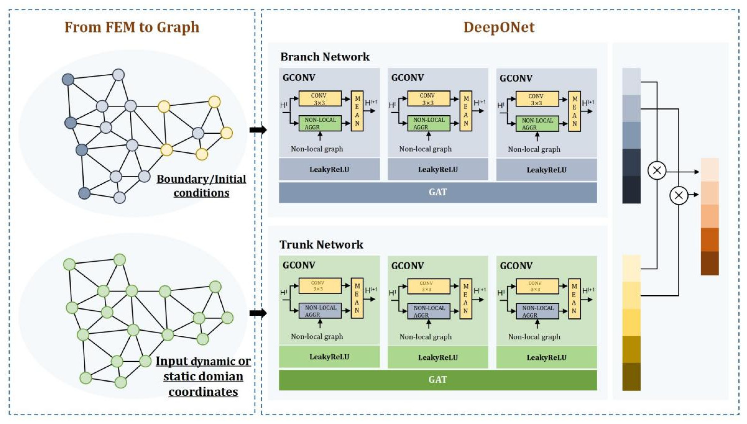
In structural strength analysis, high-fidelity numerical solutions—particularly for strongly nonlinear problems—typically require significant computational and storage resources. The propagation of graph-based simulation networks relies directly on discretized representations such as computational grids or particles (i.e., CAE models). Therefore, efficient GATs are essential for rapid prediction in such problems. Based on the traditional GAT, this study introduces a differential-algebraic equation constraint mechanism for precisely embedding the initial and the boundary conditions within the discretized input space of deep operators as shown in Figure 3. This approach not only provides structured input for data-driven neural network training but also establishes a topological adaptation foundation for the fusion.

In the original DeepONets framework, the architectural design of the branch and trunk networks is typically open-ended, with no strict constraints on their specific implementations. Therefore, this study embeds a graph attention neural network as the core subnet within DeepONets. The branch and trunk networks map the discrete representations of solution functions and initial/boundary conditions, respectively, into a shared latent variable space of graph structures. The implementation details are as follows:

• Branch Network Input: Graph-structured representations of boundary conditions $G_b$ and initial conditions $G_i$, where non-boundary nodes have zero features.
• Trunk Network Input: Graph-structured representations of Euclidean spatial coordinates, where node features consist of spatial coordinates $\mathrm{x}$, and edge features retain topological connectivity information required for field discretization.
• Operator Network Output: The physical field variable $\mathrm{u}$, whose latent space is a sequence of graph structures $Z=\{z_1,z_2,\dots ,z_{\mathrm{N}}\}$, with $z_{\mathrm{i}}$ representing latent variables obtained via graph dot product operations.

Through graph attention neural network propagation, the operator network generates predicted outputs $\widehat{\mathbf{u}}$ for the field variable $\mathbf{u}$. The trunk network $\mathcal{T}$ is expressed as:

$$\mathcal{T}\left(\mathbf{x}\right)={\mathbf{h}}_{\mathrm{geo}},$$

(11)

where ${\mathbf{h}}_{\mathrm{geo}}$ denotes latent variables encoding structural geometric features. The branch network $\mathcal{B}$ is expressed as:

$$\mathcal{B}(G_b,G_i)={\mathit{h}}_{\mathit{bc}},$$

(12)

where ${\mathit{h}}_{\mathit{bc}}$ represents latent variables encoding boundary/initial conditions. The latter part of the operator network takes the dot product of trunk and branch network latent variables as input:

$$\mathcal{O}({\mathbf{h}}_{\mathrm{geo}},{\mathit{h}}_{\mathit{bc}})=\stackrel{\mathbf{ˆ}}{\mathbf{u}},$$

(13)

where $\mathcal{O}$ denotes the graph dot product operation.

This study adopts the inherent mesh topology from FEA. For node feature extraction, an undirected graph $G=(V,E)$ includes a node set $V$ corresponding to FE mesh nodes and an edge set $E$ connecting nodes that share at least one element. Research shows that feature encoding in graph neural networks significantly impacts model performance [44]. Therefore, initial conditions are not directly used as input features. Instead, for structural analysis problems, the input node features are derived from the initial load vector $\mathbf{F}$. A load vector field is constructed via interpolation and evaluated at graph nodes. The input feature encoding for the graph can be expressed as:

$${\mathbf{f}}_i=\sum _{j=1}^M\varphi (\Vert {\mathbf{r}}_{ij}\Vert )\cdot {\mathbf{F}}_j,$$

(14)

$$\varphi (\Vert {\mathbf{r}}_{ij}\Vert )=\mathrm{e}\mathrm{x}\mathrm{p}\left(-{\displaystyle \frac{\Vert {\mathbf{r}}_{ij}{\Vert }^2}{2{\sigma }^2}}\right),$$

(15)

$$\Vert {\mathbf{r}}_{ij}\Vert =\alpha \cdot d_{\mathrm{point}}+(1-\alpha )\cdot d_{\mathrm{line}},$$

(16)

$$d_{\mathrm{line}}={\displaystyle \frac{|{\mathbf{F}}_j\cdot {\mathbf{r}}_{ij}|}{\Vert {\mathbf{F}}_j\Vert }},$$

(17)

where $\varphi (\Vert {\mathbf{r}}_{ij}\Vert )$ is a radial basis function (e.g., Gaussian kernel) weighting distance effects; ${\mathbf{r}}_{ij}$ is the coordinate offset of node $i$ relative to load point $j$; $\Vert {\mathbf{F}}_j\Vert$ is the magnitude of the load vector; $\mathsf{\alpha }$ is a weighting coefficient balancing point-to-point and point-to-line distances; $\sigma$ is a scaling hyperparameter for line distance.

This encoding method compresses high-dimensional load vector field information into low-dimensional node features through a geometry-physics coupled weighting strategy. It preserves the topological properties of FEA grids—including point-to-point distance, point-to-line distance, directional metrics, and initial load magnitude—while flexibly adapting to different scenarios via hyperparameters, thereby providing high-fidelity input representations for graph neural network-based physical field predictions.

3.2. Physical Enriched Geometric Embedding DeepONet

Based on the Geometric Embedding DeepONet, physical information is suggested to enrich structural analysis. Therefore, PINNsare introduced. PINNs integrate observational data and PDE constraints into the loss function of neural networks. Through Automatic Differentiation (AD), PDEs are embedded as soft constraints—regardless of input dimensionality, AD requires only one forward pass and one backward pass to compute all partial derivatives. Consider a parametric PDE:

$$\mathcal{N}(u;\mu )=0 \mathrm{i}\mathrm{n} \Omega \left(\mu \right),$$

(18)

where $u$ is the physical field to be solved; $\Omega \left(\mu \right)$ is the problem domain; $\mu$ represents equation parameters; $\mathcal{N}$ is the differential operator.

Sequentially, PI-DeepONets unify PINNs and DeepONets through data-physics co-optimization, efficiently solving parametric PDEs. By embedding physical constraints into operator learning, this approach enforces consistency between DeepONet outputs and governing laws, accelerating convergence and enhancing predictive accuracy. A neural network $\widehat{u}(x;\theta )$ is constructed, where $\theta =\{W,b\}$ denotes trainable weights and biases, and $\mathsf{\sigma }$ represents nonlinear activation functions. Given training data ${\mathcal{D}}_{\mathrm{data}}$ and PDE residual points ${\mathcal{D}}_{\mathrm{PDE}}$, the total loss function combines weighted contributions from data and PDE constraints:

$$\mathcal{L}\left(\theta \right)={\lambda }_{\mathrm{data}}{\mathcal{L}}_{\mathrm{data}}\left(\theta \right)+{\lambda }_{\mathrm{PDE}}{\mathcal{L}}_{\mathrm{PDE}}\left(\theta \right)+{\lambda }_{\mathrm{IC}/\mathrm{BC}}{\mathcal{L}}_{\mathrm{IC}/\mathrm{BC}}\left(\theta \right),$$

(19)

$${\mathcal{L}}_{\mathrm{data}}(\theta )={\displaystyle \frac{1}{N_{\mathrm{data}}}}\sum _{i=1}^{N_{\mathrm{data}}}{‖\widehat{u}(x_i;\theta )-u_i‖}^2,$$

(20)

$${\mathcal{L}}_{\mathrm{PDE}}(\theta )={\displaystyle \frac{1}{N_{\mathrm{PDE}}}}\sum _{j=1}^{N_{\mathrm{PDE}}}{‖\mathcal{N}\left(\widehat{u}\right(x_j;\theta );\mu )‖}^2,$$

(21)

$${\mathcal{L}}_{\mathrm{IC}/\mathrm{BC}}(\theta )={\displaystyle \frac{1}{N_{\mathrm{IC}/\mathrm{BC}}}}\sum _{k=1}^{N_{\mathrm{IC}/\mathrm{BC}}}{‖\mathcal{B}\left(\widehat{u}\right(x_k;\theta );\mu )‖}^2$$

(22)

where ${\lambda }_{\mathrm{data}}$, ${\lambda }_{\mathrm{PDE}}$, and ${\lambda }_{\mathrm{IC}/\mathrm{BC}}$ are weighting coefficients balancing loss terms; ${\mathcal{D}}_{\mathrm{PDE}}$ and ${\mathcal{D}}_{\mathrm{data}}$ are point sets sampled from the domain; ${\mathcal{D}}_{\mathrm{IC}}$ and ${\mathcal{D}}_{\mathrm{BC}}$ are point sets sampled at initial/boundary locations.

The optimal parameters ${\theta }^{\ast }$ are obtained by minimizing $\mathcal{L}\left(\theta \right)$, ensuring $\widehat{u}(x;{\theta }^{\ast })$ approximates the true solution $u\left(x\right)$.

The Graph-Structured PI-DeepONet (GS-PI-DeepONet) integrates GNNs, DeepONets, and PINNs to address unstructured geometric problems in parametric structural analysis as shown in Figure 4. Its core innovation lies in embedding physical fields and their governing equations into graph-structured feature learning, leveraging non-Euclidean topology modeling to overcome limitations of traditional mesh-based methods in complex geometries, nonlinearities, and multiphysics coupling.

3.3. Boundary Conditions Enforcement in GS-PI-DeepONet

In the GS-PI-DeepONet framework, boundary conditions are enforced through a combination of a hard-constraint ansatz integrated into the operator network’s output and soft-constraint penalties in the physics-informed loss function.

Hard Constraints via Solution Ansatz

The core idea is to structure the output of the operator network $\mathrm{O}$ to automatically satisfy the essential (geometric) boundary conditions. The raw prediction $\widehat{u}\left(x\right)$ from the DeepONet is not the final solution but is transformed into a function that inherently fulfills the BCs.

The final solution $u_{\mathit{pred}}\left(x\right)$ is constructed as:

$$u_{\mathit{pred}}\left(x\right)=B\left(x\right)+T\left(x\right)\cdot \widehat{u}\left(x\right)$$

(23)

where $\widehat{u}\left(x\right)=O({\mathbf{h}}_{\mathrm{geo}},{\mathit{h}}_{\mathit{bc}})$ is the output of the Graph-Structured DeepONet operator network, $B\left(x\right)$ is a function chosen to satisfy the non-homogeneous essential boundary conditions. For homogeneous BCs, $B\left(x\right)=0$, $T\left(x\right)$ is a smooth lifting function that is zero at the locations where essential BCs are applied, Ensuring the network’s output $\widehat{\mathrm{u}}\left(x\right)$ does not violate them.

For example, application to a Cantilever Beam (Fixed at $x=0$) as shown in Section 6.1 can be expressed as follows.

The essential boundary conditions are:

$$u\left(0\right)=0,u^{\prime }\left(0\right)=0$$

(24)

A suitable lifting function that satisfies $T\left(0\right)=0$ and $T^{\prime }\left(0\right)=0$ is:

$$T\left(x\right)=x^2$$

(25)

with homogeneous BCs, $B\left(x\right)=0$. Therefore, the final solution ansatz used to calculate derivatives and the loss is:

$$u_{\mathrm{pred}}\left(x\right)=x^2\cdot \widehat{u}\left(x\right)$$

(26)

This formulation guarantees that $u_{\mathrm{pred}}\left(0\right)=0$ and $u_{\mathrm{pred}}^{\prime }\left(0\right)=0$, no matter what the network outputs for $\widehat{u}\left(x\right)$ are.

Soft Constraints via Physics-Informed Loss

The natural (force) boundary conditions and the governing PDE itself are enforced as soft constraints by embedding them directly into the loss function, as defined in Equations (19)–(22).

For the cantilever beam example (free at $x=L$), the natural boundary conditions are zero moment and zero shear:

$$u^{″}\left(L\right)=0,u^{‴}\left(L\right)=0$$

(27)

These are incorporated into the loss term ${\mathcal{L}}_{\mathrm{IC}/\mathrm{BC}}$. The total physics-informed loss function becomes:

$$\mathcal{L}\left(\theta \right)={\lambda }_{\mathrm{data}}{\mathcal{L}}_{\mathrm{data}}\left(\theta \right)+{\lambda }_{\mathrm{PDE}}{\mathcal{L}}_{\mathrm{PDE}}\left(\theta \right)+{\lambda }_{\mathrm{IC}/\mathrm{BC}}{\mathcal{L}}_{\mathrm{IC}/\mathrm{BC}}\left(\theta \right)$$

(28)

where ${\mathcal{L}}_{\mathrm{PDE}}\left(\theta \right)$ penalizes the violation of the Euler-Bernoulli equation $\mathrm{E}\mathrm{I}{\displaystyle \frac{{\mathrm{d}}^4{\mathrm{u}}_{\mathrm{pred}}}{\mathrm{d}{\mathrm{x}}^4}}=q(x)$ at collocation points inside the domain, ${\mathcal{L}}_{\mathrm{IC}/\mathrm{BC}}(\theta )$ now includes penalties for the natural BCs at $x=L$:${\mathcal{L}}_{\mathrm{IC}/\mathrm{BC}}(\theta )={\displaystyle \frac{1}{{\mathrm{N}}_{\mathrm{BC}}}}{\sum }_{\mathrm{k}=1}^{{\mathrm{N}}_{\mathrm{BC}}}\left[{\left|u_{\mathrm{pred}}^{″}(L)\right|}^2+{\left|u_{\mathrm{pred}}^{‴}(L)\right|}^2\right]$. All derivatives $({\mathrm{u}}_{\mathrm{pred}}^{″},{\mathrm{u}}_{\mathrm{pred}}^{‴},{\displaystyle \frac{{\mathrm{d}}^4{\mathrm{u}}_{\mathrm{pred}}}{\mathrm{d}{\mathrm{x}}^4}})$ are computed from the ansatz ${\mathrm{u}}_{\mathrm{pred}}(\mathrm{x})={\mathrm{x}}^2\cdot \widehat{\mathrm{u}}(\mathrm{x})$ using automatic differentiation.

Generally, in the suggested framework:

Hard Constraints (Ansatz): Essential BCs $\left(u\right(0)=0,u^{\prime }(0)=0)$ are enforced exactly by defining the final solution as $u_{\mathit{pred}}\left(x\right)=x^2\cdot \widehat{u}\left(x\right)$.

Soft Constraints (Loss Function): The governing PDE and natural BCs $\left(u^{″}\right(L)=0,u^{‴}(L)=0)$ are enforced by minimizing their residuals, which are calculated from the hard-constrained solution $u_{\mathit{pred}}\left(x\right)$.

This hybrid approach ensures strict adherence to geometric constraints while allowing the model to learn the physics and force-boundary conditions from data, which is a hallmark of the GS-PI-DeepONet method.

4. Evaluation Metrics

The primary goal of this work, which involves modeling the input–output relationship of a structural analysis system, is to learn the mapping from an input function to an output function. Consequently, the underlying evaluation paradigm is that of a regression problem. The most common performance metrics for regression models are Mean Squared Error (MSE), Mean Absolute Error (MAE), Coefficient of Determination (R²), and Relative Error (RE).

The R² quantifies the proportion of the variance in the observed data that is captured by the model. In deep operator neural networks, R² is frequently used to assess how well the network approximates the overall nonlinear governing equations. The formula is

$$R^2=1-{\displaystyle \frac{{\sum }_{i=1}^n(y_i-{\widehat{y}}_i{)}^2}{{\sum }_{i=1}^n(y_i-\bar{y}{)}^2}},$$

(29)

where $y_i$ is the true value for the $\mathrm{i}$-th test sample, ${\widehat{y}}_i$ is the corresponding prediction from the regression model, $\bar{y}$ is the mean of the observed values, and $n$ is the number of samples. The numerator, ${\sum }_{i=1}^n(y_i-{\widehat{y}}_i{)}^2$, resembles the Mean Squared Error (MSE), while the denominator, ${\sum }_{i=1}^n(y_{\mathrm{i}}-\bar{y}{)}^2$, is analogous to the variance (Var). $R^2$ ranges from $-\mathrm{\infty }$ to 1. A value close to 1 indicates that the model explains a large proportion of the variability in the target variable, implying a high goodness-of-fit. Conversely, values near 0 or negative suggest the model performs poorly—sometimes even worse than simply predicting the mean for each sample—often pointing to severe overfitting or a fundamental design flaw. When applied to nonlinear regression tasks, $R^2$ provides a concise summary of the model’s ability to approximate complex function mappings. Its limitations are that it is sensitive to outliers and does not directly measure generalization capability.

The RE is a widely used metric that gauges the discrepancy between a predicted value (or numerical solution) and the ground truth. It combines the concepts of the Euclidean norm and relative error, and it uses a squaring operation to amplify the influence of large individual errors. The metric is especially suitable for multi-dimensional data or vector-valued outputs. The formula is

$$\mathrm{Relative} \mathrm{Error}={\displaystyle \frac{\Vert y-\widehat{y}{\Vert }_2}{\Vert y{\Vert }_2}},$$

(30)

where $y-\widehat{y}{\Vert }_2$ denotes the Euclidean distance (2-norm) between the true and predicted vectors, and $\Vert \mathrm{y}{\Vert }_2$ is the $L_2$ (2-norm, Euclidean length) of the true vector, defined as

$$\Vert v{\Vert }_2=\sqrt{\sum _{j=1}^d{v}_j^2}.$$

(31)

In practice, the relative error $L_2$ typically lies between 0 and 1. A value exceeding 1 indicates that the prediction error is larger than the magnitude of the true value itself, usually signifying poor model performance. Smaller relative errors $L_2$ imply closer agreement between predictions and observations. A practical caveat: if the true vector contains very small components (values close to zero), the denominator may become extremely small, causing the relative error to become inflated. Such cases should be handled with appropriate preprocessing or thresholding.

5. Numerical Example Descriptions

This section provides a brief and thorough summary of the numerical experiments performed. The entire codebase for these experiments was developed using Python 3.13, with the deep-learning components being constructed using PyTorch version 1.12. Both the training and inference processes were efficiently executed on a single NVIDIA GTX 4090 GPU.

In terms of dataset generation, the benchmark training data were generated by a second-order finite-difference solver, while the training data for real case 1 and case 2 were produced using FEM solver. Regarding the network architecture, the overall model consists of a branch net and a trunk net, both of which are built upon GAT. The branch net has an input tensor shape of (dataset_size, n_nodes, m), where dataset_size represents the number of training samples, n_nodes denotes the number of graph nodes, and m signifies the parameter dimension. The trunk net, on the other hand, has an input tensor shape of (dataset_size, coordinate_dimension). This detailed description provides a clear understanding of the experimental setup and methodology employed in the numerical experiments. Attention coefficients were normalized with LeakyReLU (negative_slope = 0.2, the PyTorch default). Every learnable weight was initialized with the Kaiming uniform initializer to mitigate vanishing/exploding gradients. The activation function after every hidden layer is tanh. The optimizer chosen for this project is Adam, with a learning rate of 1 × 10⁻⁴ and all other hyperparameters left at their PyTorch defaults. The batch size used is 4. These hyperparameters were obtained through extensive grid-search and have proven to be stable on both the training and validation sets, demonstrating strong robustness against distributional shifts. The hyperparameters in all cases are show in

Table 1. Hyperparameter list.

Hyper-Parameter	Benchmark	Case 1	Case 2
Branch Net
Input feature dim	100	1	1
Hidden layer sizes	(40, 2)	(256, 2)	(256, 2)
Attention heads	—	4	4
Output feature dim	1	1	1
Trunk Net
Input feature dim	1	3	3
Hidden layer sizes	(40, 2)	(256, 2)	(256, 2)
Attention heads	—	4	4
Edge index	—	(2, 16,500)	(2, 101,690)
Output feature dim	1	1	1
Training
Training samples	150	1000	1000
Epochs	30,000	60,000	60,000
Learning rate	1 × 10−3	1 × 10−4	1 × 10−4
Model-save frequency	1000	1000	1000
Batch size	16	4	4
Posterior sampling
Sample count	1000	200	200

.

6. Analytical Solutions and Simulation Error Analysis

To evaluate the accuracy of the suggested method, two benchmark problems with analytical solutions were selected: the cantilever beam under uniform load and the Hertz contact problem. The detailed solution processes and evaluation metrics are as follows.

6.1. Cantilever Beam Under Uniform Load Problem

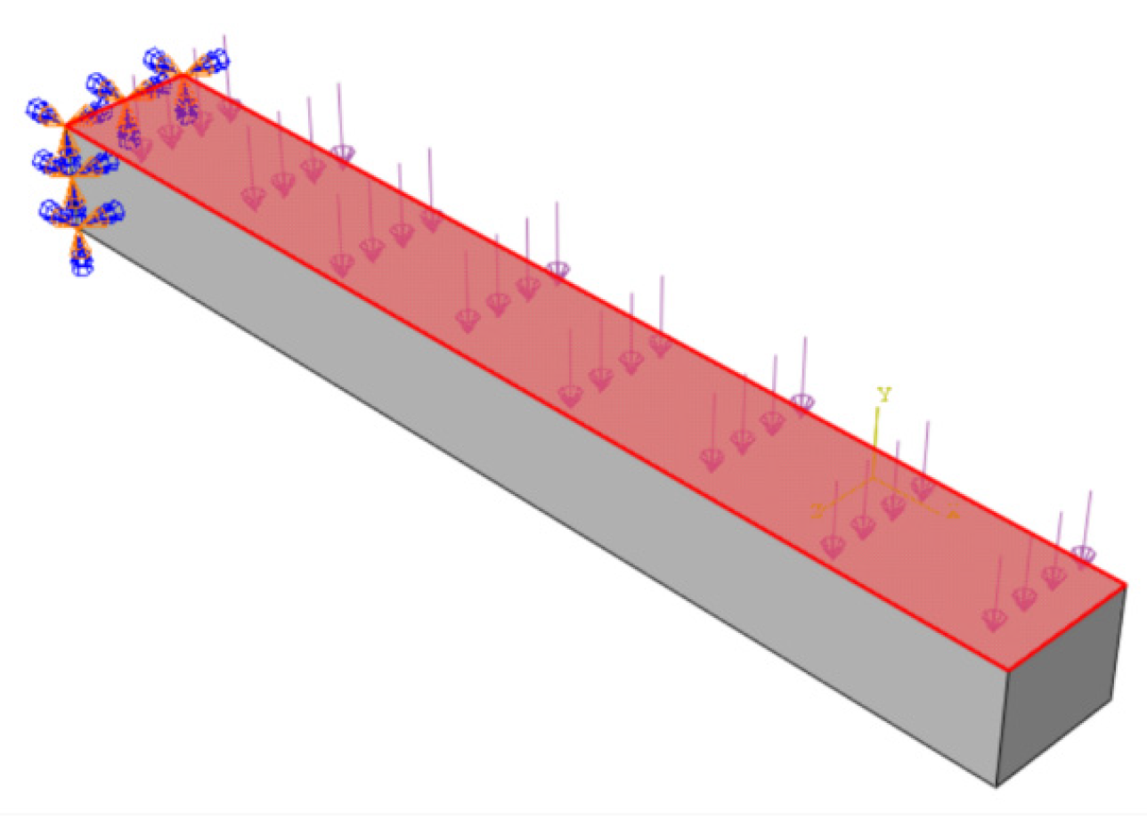
A three-dimensional cantilever beam is fixed at one end and subjected to a uniform load $\mathrm{w}$ on its top surface as shown in Figure 1. The deflection of the cantilever beam follows the Euler–Bernoulli beam equation:

$$EI{\displaystyle \frac{d^{4}v}{d{x}^4}}=q(x)$$

(32)

The analytical solution for the deflection $v$(x) of the beam is given by:

$$v(x)={\displaystyle \frac{w{x}^2}{24EI}}(6l^2-4lx+x^2);$$

(33)

where $x$ denotes distance from the fixed end, $I$ denotes length of the beam, E is Young’s modulus and I is moment of inertia of the cross-section. For a rectangular cross-section, the moment of inertia is:

$$I={\displaystyle \frac{b{h}^3}{12}}$$

(34)

where b represents the width of the cross-section and h denotes the height of the cross-section. For this problem, Young’s modulus (E) is 209,000 Pa, the beam length (l) is 200 m, the cross-section width (b) is 25 m, the cross-section height (h) is 20 m, the applied uniform pressure (p) is 0.5 Pa, and the equivalent 2D uniform load (w) is calculated as p multiplied by b, which equals 12.5 Pa.

In system identification problems, the design quality of the input $q\left(x\right)$ directly determines the theoretical best accuracy of the model. If the input signal fails to adequately cover the key dynamic range of the system or contains redundant or missing information, the model’s accuracy will inevitably be limited. Therefore, this study primarily considers sampling from a Gaussian Random Field (GRF) in function space, using a zero-mean Gaussian Random Field:

$$q\left(x\right)\sim \mathcal{G}\mathcal{P}(0,k(x,x^{\prime }\left)\right)$$

(35)

where the covariance kernel function $k(x,x^{\prime })$ is a Radial Basis Function (RBF) kernel with a length scale parameter $\mathrm{l}$. The length scale $\mathrm{l}$ determines the smoothness of the sampled functions—the larger $\mathrm{l}$, the smoother $q\left(x\right)$.

From the Gaussian random field of length $L$, 1150 sets of distributed load functions $q\left(x\right)$ are sampled with a resolution of $\Delta x$. The differential equation is solved using a second-order implicit finite difference method to obtain reference solutions for each $q\left(x\right)$ at $N$ positions. This example involves simple one-dimensional data, and the suggested method is employed for the solution. The input to the branch network is the function $q\left(x\right)$, with a shape of (150, 100). The input to the trunk network is the position information $x$ of the values, with a shape of (100, 1). The output is the $v\left(x\right)$ values at different positions for different functions $q\left(x\right)$.

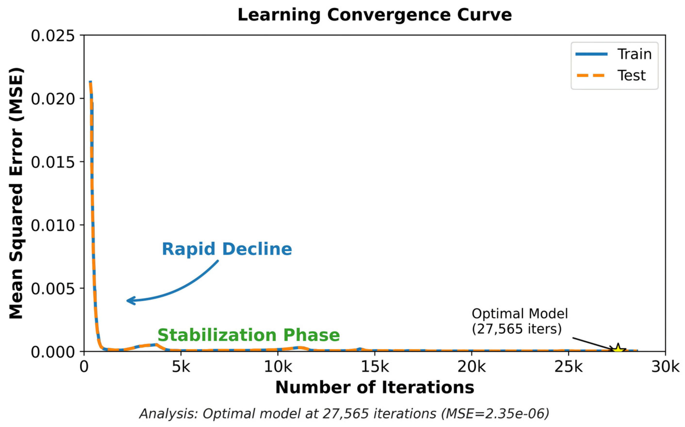
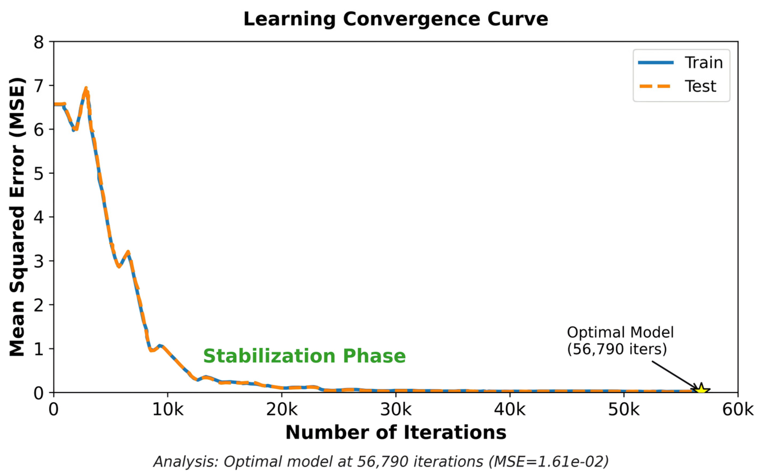
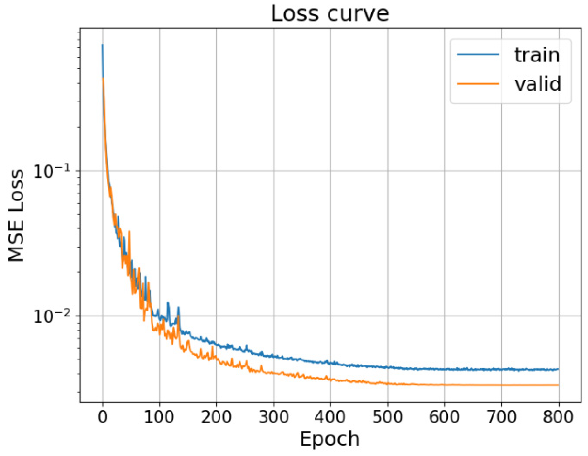
In this example, 150 sets of data points are used for training, and 1000 sets are used for testing. Figure 5 shows the convergence curves of the training loss, testing loss, and testing evaluation metrics (MSE) during the model training process. The overall convergence speed of the training and testing datasets is fast, with small errors, and the MSE of the testing set decreases synchronously, indicating that the model gradually improves its generalization performance and numerical prediction accuracy during training.

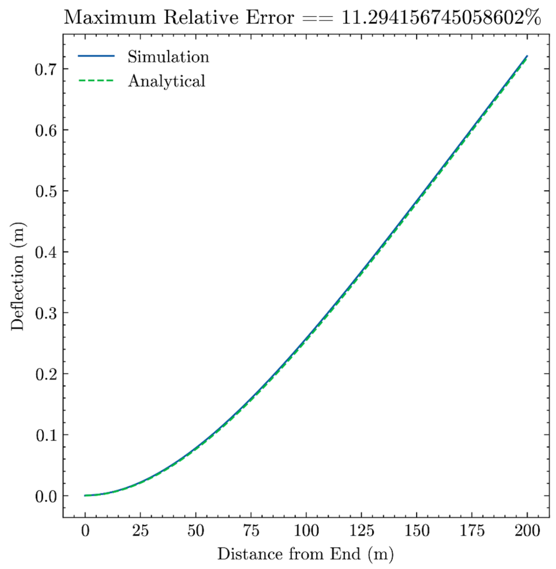
Moreover, the deflection of the top surface from the simulation closely matches the analytical solution as shown in Figure 6, where the blue solid and green dot lines represent the reference solution and the GS-PI-DeepONets prediction results, respectively. It can be observed that the deflection of the top surface from the simulation matches the analytical solution for a cantilever beam almost exactly.

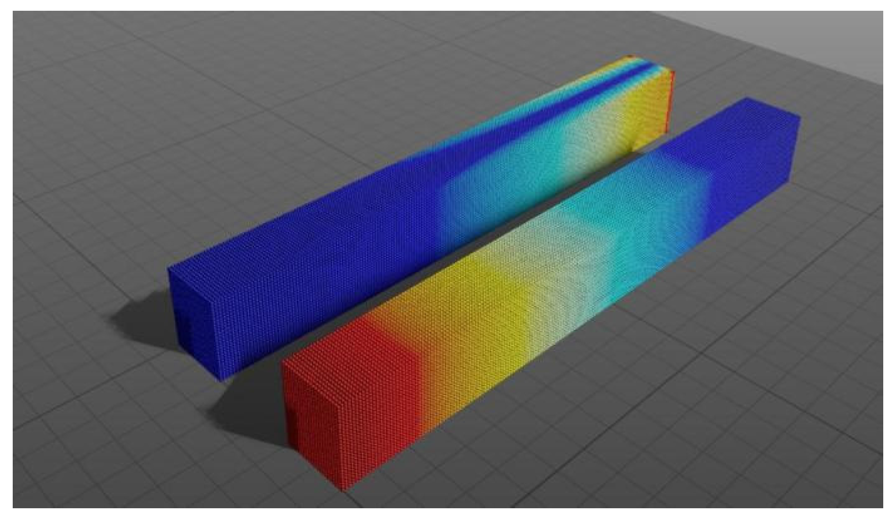
The simulation predicted by the suggested method results are shown in Figure 7. The results of various solution methods are presented

Table 2. Performance metrics for the cantilever beam bending problem.

Prediction Field	Metric	GS-PI-DeepONets
		In-Distribution	Out-Distribution
$w\left(x\right)$	Mean $R^2$	0.9998	0.9907
	Mean relative $L_2$ error	0.0925	0.0949
	Data generation time (s)	3.318
	Training time (s)	3.71
	Solution time (s)	0.2589

. In addition to relative $L_2$ error, $R^2$ other metrics are also used to evaluate the outcomes. For the in-distribution testing set, the $R^2$ values are as high as 0.9999, with a relative $L_2$ error of 5.45 × 10⁻². Meanwhile, the method also performs effectively in predictions for out-of-distribution samples. To illustrate this, a new testing dataset is constructed where the input functions are sampled from a Gaussian Random Field with a specified length scale ${\mathrm{l}}^{\prime }$. In this testing set, the model achieves an average $R^2$ of 0.9907 and a relative $L_2$ error of 6.49 × 10⁻² across 1000 test samples. The results demonstrate that the predictions of GS-PI-DeepONets exhibit excellent agreement with the reference solutions.

6.2. Hertz Contact Problem

A cylindrical roller is placed on a rectangular block. A uniform line load $F_n$ is applied to the roller, while the block’s bottom surface is fixed as shown in Figure 8. The contact is assumed to be frictionless.

The Hertz contact theory provides the analytical solution for contact pressure:

$$p(x)={\displaystyle \frac{2F_n}{\pi b}}\sqrt{1-{\left({\displaystyle \frac{x}{b}}\right)}^2}$$

(36)

where $F_n$ denotes applied load per unit length, $\mathrm{b}$ denotes half-width of the contact area, E′ denotes combined Young’s modulus, R′ denotes the combined radius and is defined as:

$${\displaystyle \frac{1}{E^{\prime }}}={\displaystyle \frac{1-{\nu }_1^2}{E_1}}+{\displaystyle \frac{1-{\nu }_2^2}{E_2}}$$

(37)

$${\displaystyle \frac{1}{R^{\prime }}}={\displaystyle \frac{1}{R_1}}+{\displaystyle \frac{1}{R_2}}$$

(38)

where E₁ and E₂ represent the Young’s module of the roller and block, respectively, ν₁ and ν₂ represent the Poisson’s ratios of the roller and block, respectively, and R₁ denotes the radius of the roller. In this problem, E₁ is 70 GPa, E₂ is 210 GPa, ν₁ and ν₂ are both 0.3, $F_n$ is 35 kN and R₁ is 50 mm.

The input to the branch network encodes the source term and/or parameters of the parametric PDE. For the Hertz contact problem, this is the applied load per unit length, $F_n$. Data Structure and Justification: Unlike the cantilever beam in 6.1 where the input was a function $q\left(x\right)$ sampled at many points, the Hertz problem is parameterized by a single scalar value $F_n$. Therefore, the branch net input is a finite-dimensional vector representing this parameter. The input to the trunk network defines the location at which the solution operator is evaluated. For the 1D Hertz contact problem, this is the spatial coordinate $x$ along the contact interface.

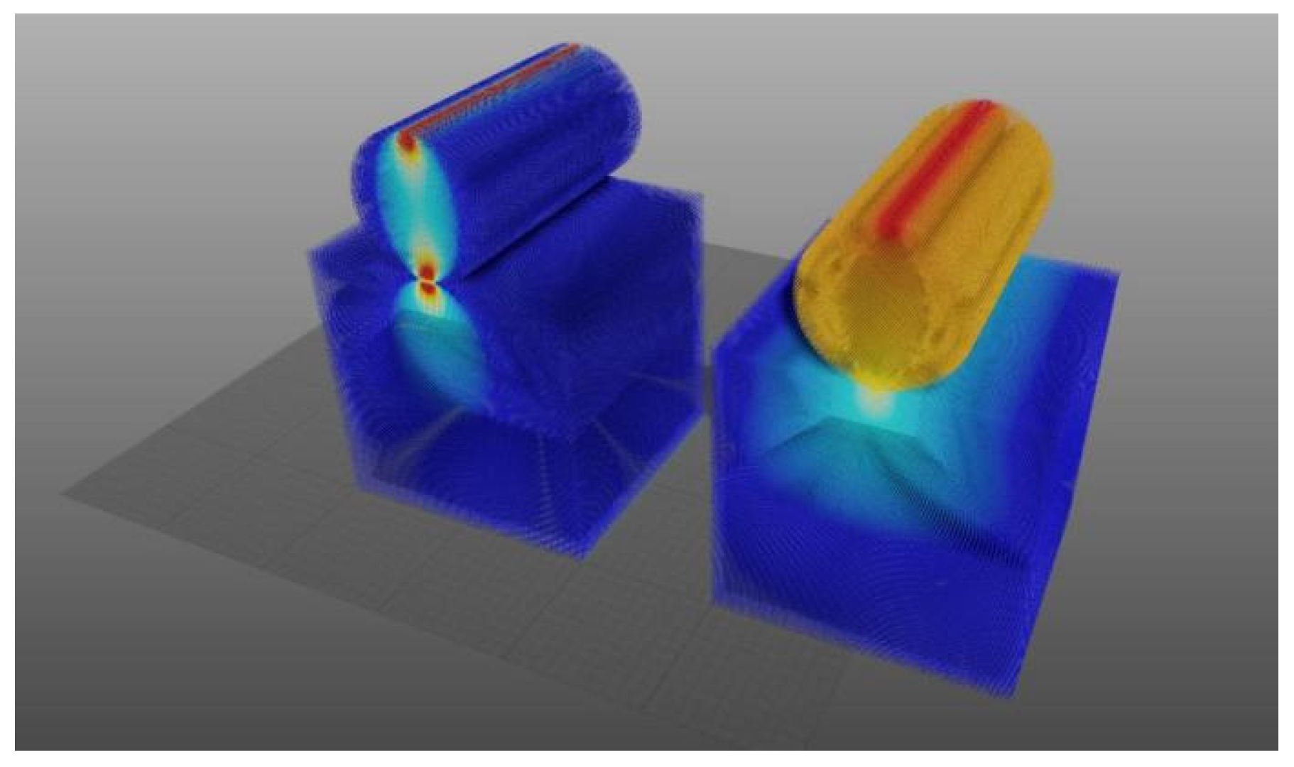
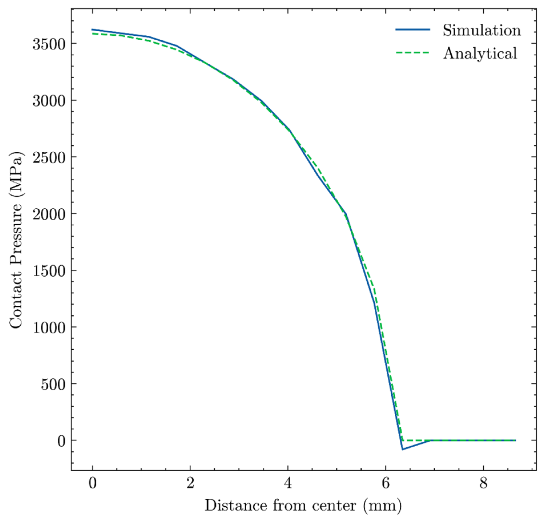
The settings of this problem are the same as those for the last one. Similar to the previous benchmark, Figure 9 shows the convergence curves of the training loss, testing loss, and testing evaluation metrics (MSE) during the model training process. The overall convergence speed of the training and testing datasets is fast, with small errors, and the MSE of the testing set decreases synchronously. The simulation predicted by the suggested method results are shown in Figure 10. The contact pressure distribution well matches the Hertz theory predictions as shown in Figure 11.

The simulation and analytical results are presented in Figure 11 and the outcomes of various solution methods are detailed in

Table 3. Performance metrics for Hertz problem.

Prediction Field	Metric	GS-PI-DeepONets
		In-Distribution	Out-Distribution
$p\left(x\right)$	Mean $R^2$	0.9878	0.9794
	Mean relative $L_2$ error	0.1345	0.2013
	Data generation time (s)	8.318
	Training time (s)	10.71
	Solution time (s)	0.2589

. For the in-distribution testing set, the R-squared $R^2$ values are as high as 0.9878, with a relative $L_2$ error of 1.345 × 10⁻¹. Meanwhile, the method also performs effectively in predictions for out-of-distribution samples. To illustrate this, a new testing dataset has been constructed where the input functions are sampled from a Gaussian random field with a specified length scale ${\mathrm{l}}^{\prime }$. In this testing set, the model achieves an average $R^2$ of 0.9794 and a relative $L_2$ error of 2.013 × 10⁻¹ across 1000 test samples. The results demonstrate that the predictions of GS-PI-DeepONets exhibit excellent agreement with the reference solutions.

7. Applications

7.1. Case 1: Stiffness Analysis of the Upper Connecting Plate in a Recliner Mechanism

Due to the installation constraints of the RTA motor in an electric automotive seat back, both the vertical and horizontal tubes of the backrest must be shortened. To maintain structural integrity, additional stiffening ribs are introduced to weld the two parts together. While the connecting plate used in both manual and electric seat backs is largely identical, an extra reinforcement plate is required for the electric version.

This section focuses on a structural analysis problem involving the upper connecting plate of the recliner mechanism. Specifically, the investigation aims to ensure that the shell structure does not deform excessively under compressive loading such that it interferes with the motor module.

The geometry of the connecting plate is illustrated in Figure 12, with the dashed line indicating the centerline of the pivot axis. The baseline dimensions are detailed as follows: the distance from the pivot axis centerline to the top of the reinforcement plate is 250 mm; the Z-direction length of the lower horizontal tube is 40 mm; the distance from the pivot axis centerline to the bottom surface of the lower horizontal tube is 85 mm; the backrest has an inward offset of 4 mm; and the lateral offset width is 10 mm. The material used for this component is 45# steel.

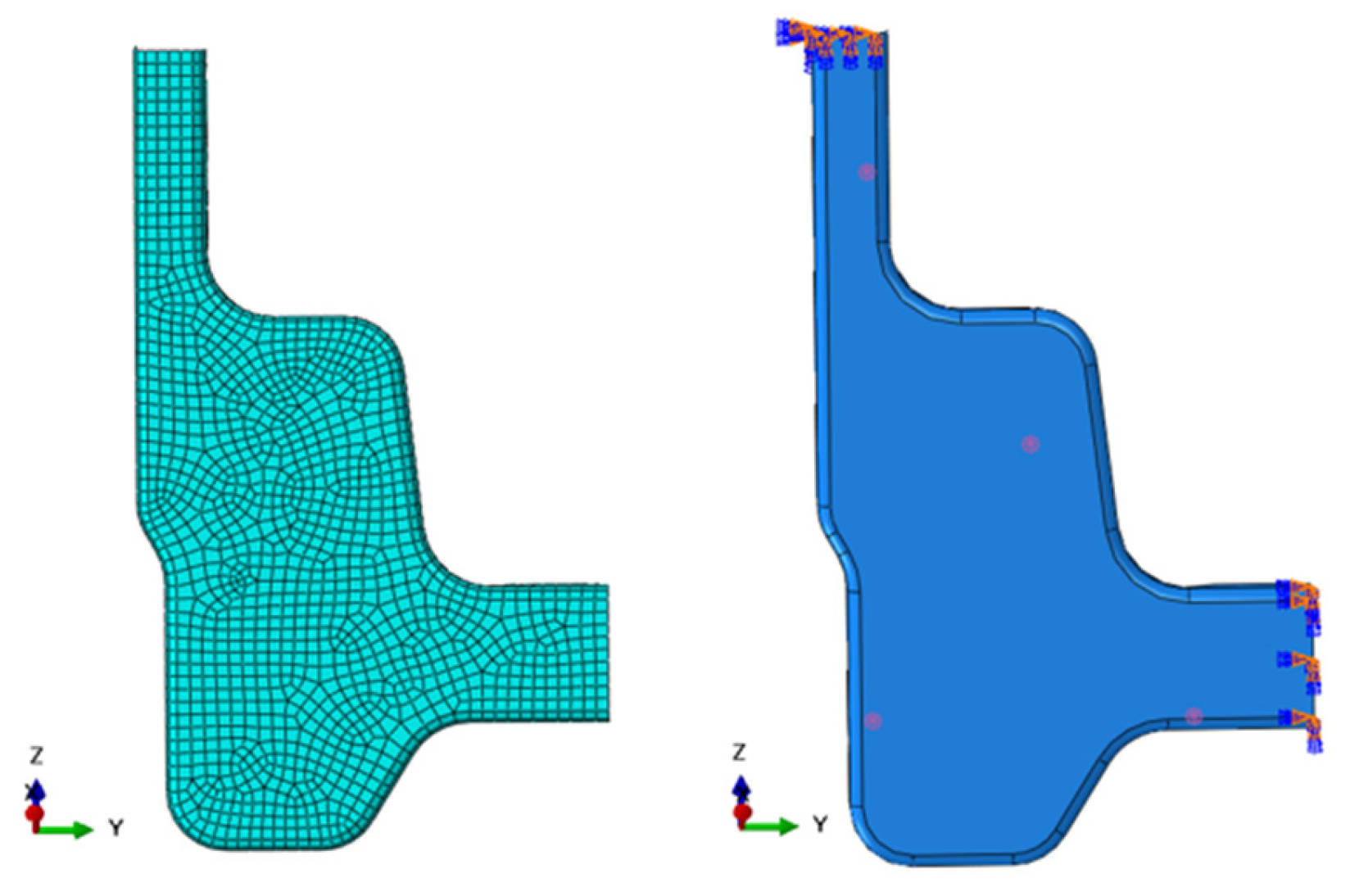
In the FE model, the upper ends of the vertical tube and the lower ends of the horizontal tube are fully fixed. A distributed load is applied across the contact surface, with the load design domain defined as (0.005, 0.5). The FE model consists of 2126 shell elements (S4R) and 2242 nodes, the shell thickness is 2 mm. The FE model with the initial and boundary conditions is shown in Figure 13.

In this case, we established two types of boundary conditions (BCs):

BC1: Uniformly distributed loads are applied to all nodes of the workpiece, each with a magnitude of 100 N. The load magnitude varied within a ±20% range.

BC2: Randomly distributed loads are applied, featuring both random placement locations and magnitude variations that matched the adjustment criteria of Boundary Condition 1, as shown in Figure 14.

Using the Latin Hypercube Sampling (LHS) method, 1200 different load cases were sampled within the parameter design space for both boundary conditions. The resolution was set accordingly, and the observed responses were obtained via FEA.

The neural network architecture comprises a branch network and a trunk network. The branch network input consists of design parameters, with a shape of (1000, 1). Meanwhile, the trunk network input includes node coordinates, labeled as node_coordinates, with a shape of (2242, 3), and edge index, labeled as edge_index, with a shape of (2, 16,500). The output of this neural network architecture is the displacement values at node locations, having a shape of (1000, 1). Regarding model training and evaluation, the dataset was divided into two parts: a training set comprising 1000 samples and a test set consisting of 200 samples.

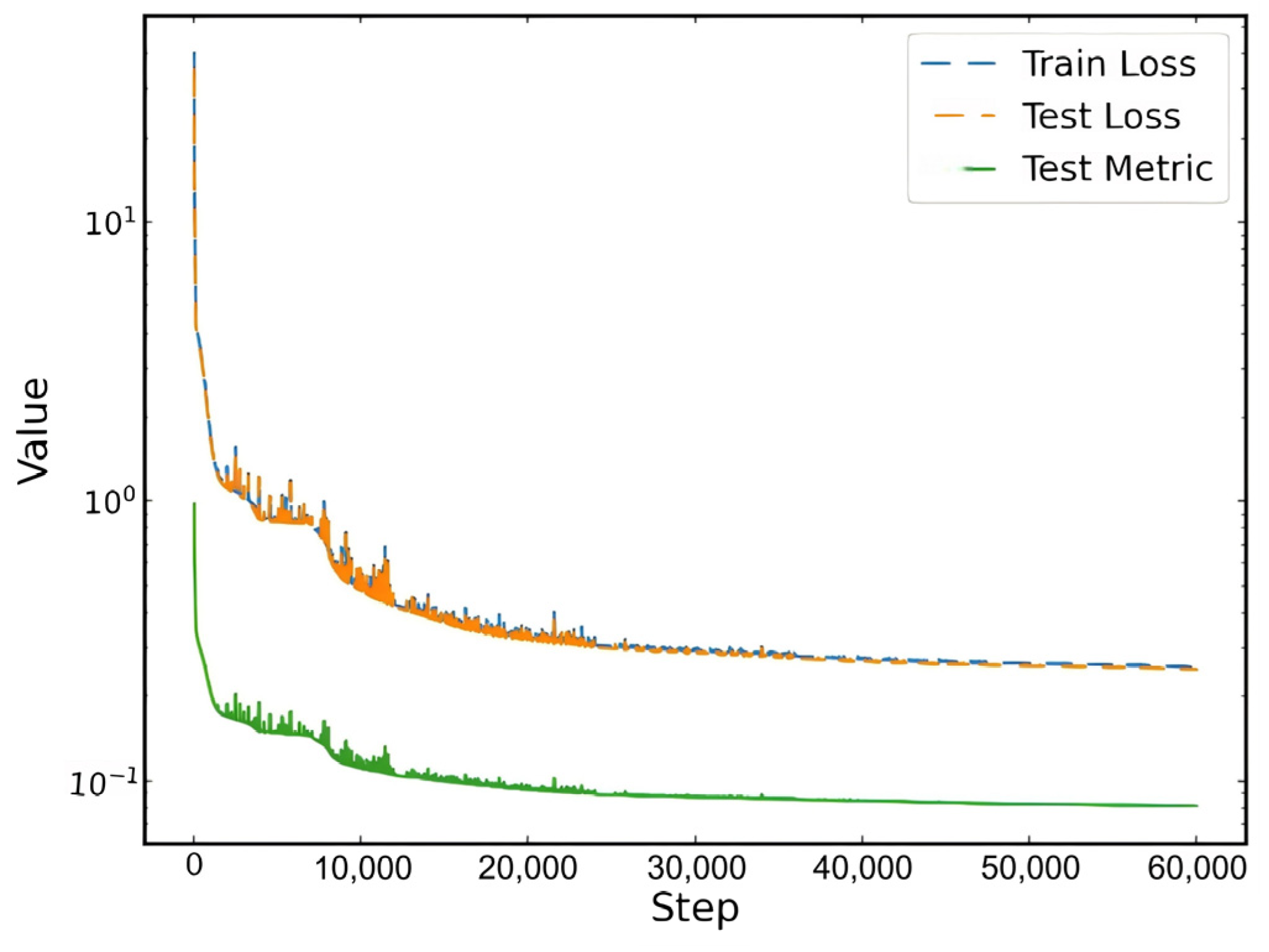
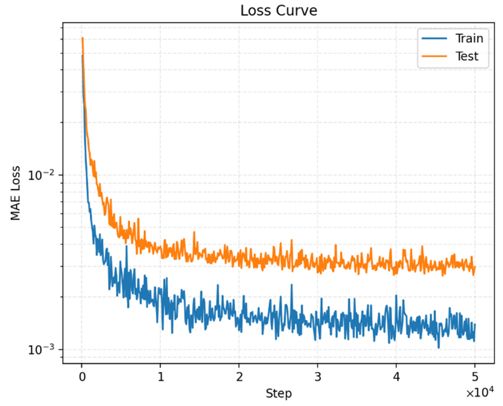
For BC1, as illustrated in Figure 15, the diagram, both training and test losses display smooth and stable convergence. The close alignment between the training and test losses signifies excellent generalization performance with no signs of overfitting.

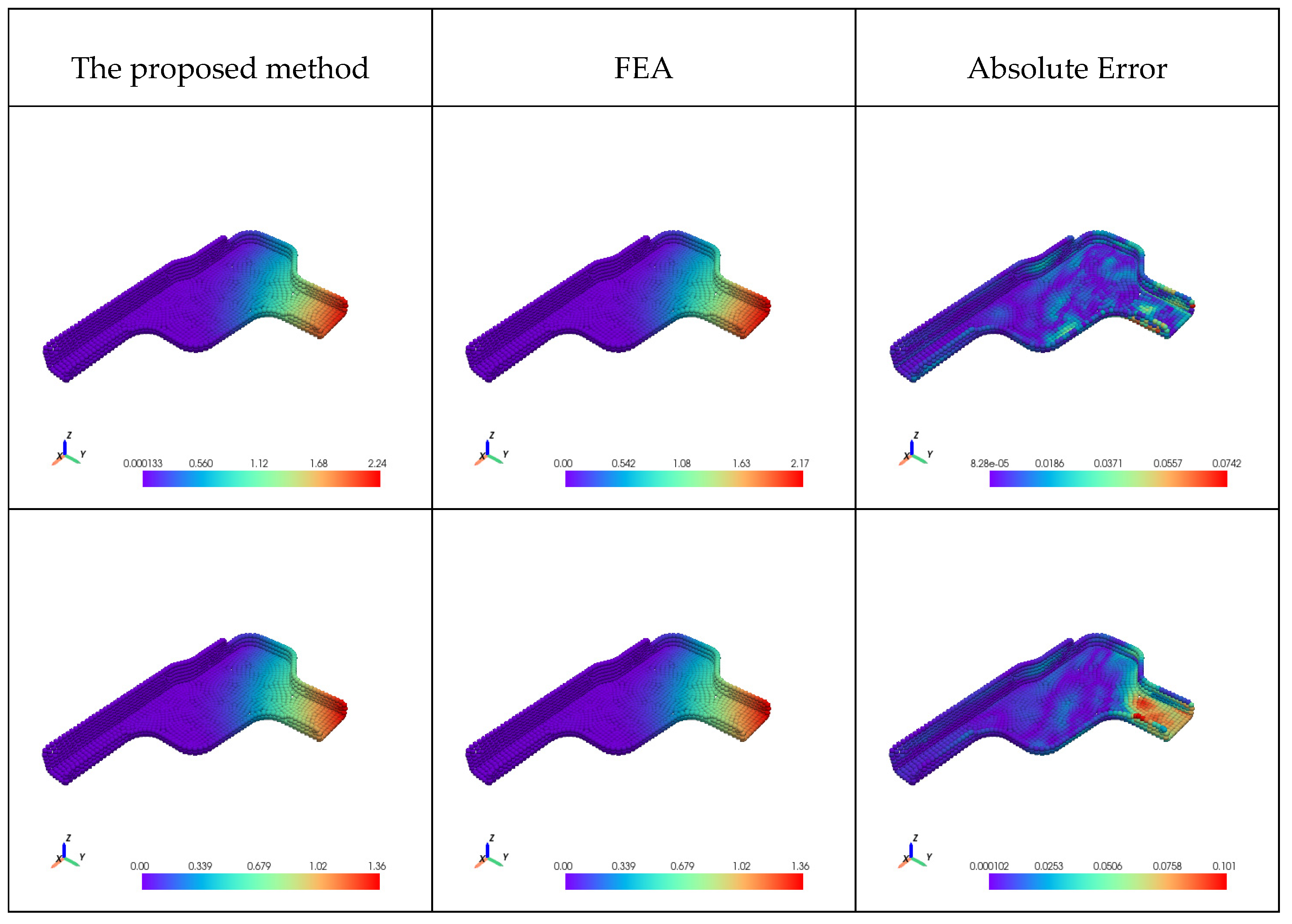
The predicted and reference displacement fields are visualized in Figure 16, arranged from left to right as: GS-PI-DeepONets prediction, FEA reference solution and test case error. From top to bottom, the samples correspond to maximum, minimum, and median relative errors, respectively. Notably, larger errors are observed near the geometric boundaries of the connecting plate.

Table 4. Performance comparison of different methods in connecting plate stiffness analysis for case 1 with BC1.

Predicted Field	Metric	FEM	GS-PI-DeepONets	DeepONets
Displacement Field	Mean R2	/	0.9832	0.9548
Displacement Field	Mean Relative $L_2$ Error	/	0.0685	0.1240
Data Generation Time (s)	Data Generation Time (s)	/	2522.8	2522.8
Training Time (s)	Training Time (s)	/	314.81	349.7
Solving Time (s)	Solving Time (s)	2.0163	0.2601	0.2823

summarizes the performance of various methods on the test set, with a Mean R² of 0.9832 and a Mean relative $L_2$ error of 6.85 × 10⁻². These metrics indicate a minimal discrepancy between the predicted and reference displacement fields. Compared to the original DeepONets, the proposed GS-PI-DeepONets method demonstrates significant improvements in both accuracy and training efficiency. Unlike simpler problems, such as cantilever beams, the deep learning approach in this case achieves much faster solution times than traditional FEM.

For the BC2, as shown in Figure 17, both training and test losses exhibit smooth and stable convergence. The close alignment between training and test losses indicates excellent generalization performance with no over-fitting. Similar to the results of case1 with BC1, the simulation results are illustrated in Figure 18 and corresponding criteria for efficiency and accuracy are listed in

Table 5. Performance comparison of different methods in connecting plate stiffness analysis for case 1 with BC2.

Predicted Field	Metric	FEM	GS-PI-DeepONets	DeepONets
Displacement Field	Mean R2	/	0.9998	0.9543
Displacement Field	Mean Relative $L_2$ Error	/	0.0296	0.0675
Data Generation Time (s)	Data Generation Time (s)	/	2532.7	2565.2
Training Time (s)	Training Time (s)	/	315.2	356.1
Solving Time (s)	Solving Time (s)	2.0163	0.2101	0.2934

. Obviously, the proposed GS-PI-DeepONets method demonstrates significant improvements in both accuracy and training efficiency.

7.2. Case 2: Strength Analysis of a Support Bracket

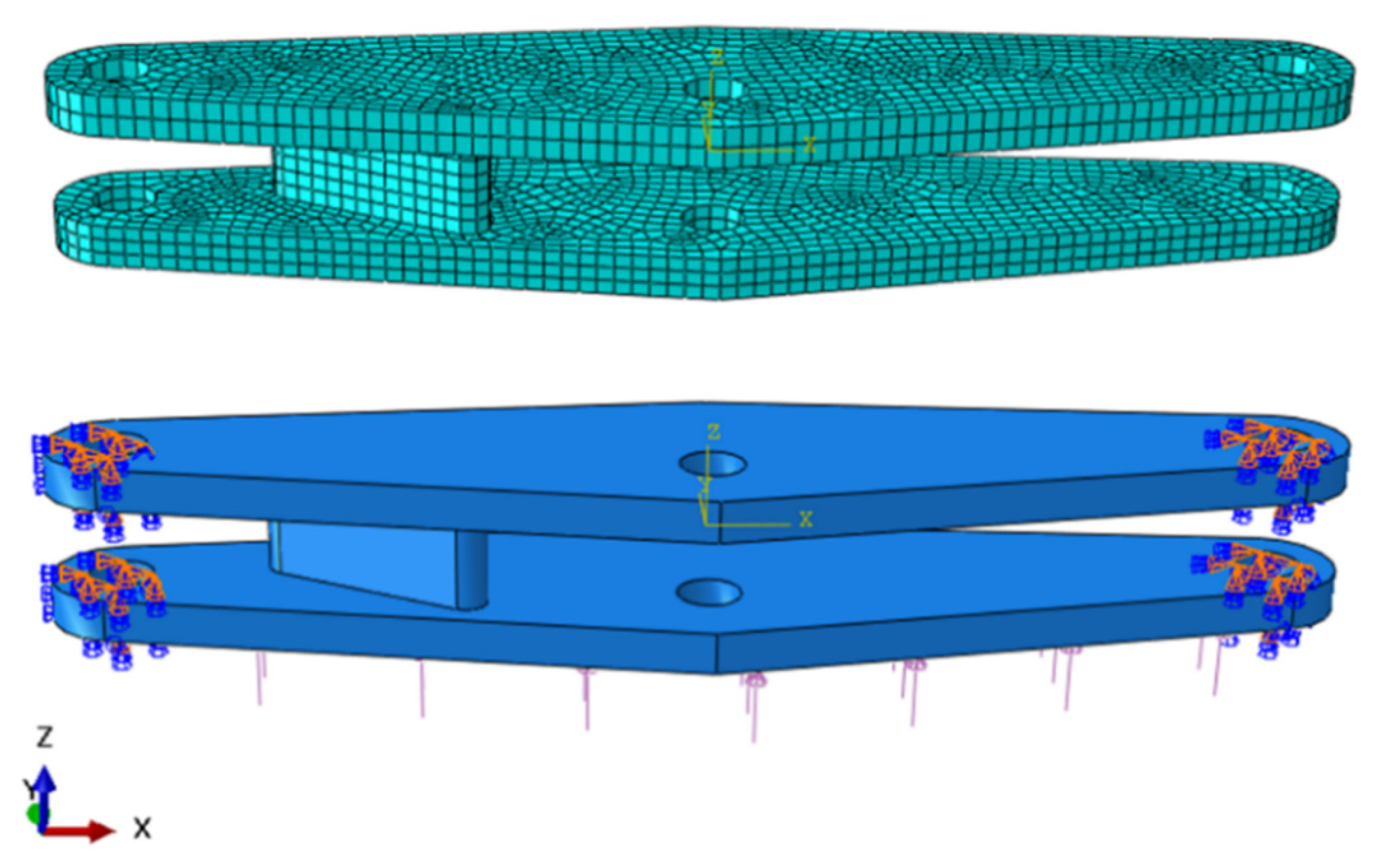
This section investigates the stress and deformation behavior of a support bracket subjected to external loading. The material utilized is 45# steel. The bolt-hole nodes of the bracket are constrained in all transitional and rotational degrees of freedom (X, Y, Z). The FE model consists of 5594 C3D8R elements and 8436 nodes. The FE model, along with its initial and boundary conditions, is illustrated in Figure 19. Similar to case 1, two BCs are considered. The first is that a uniformly distributed load 200 N is applied in the Z-direction to the lower surface of the component, where the load magnitude varied within ±20% range; the second one is to randomly generate a concentrated load different location applied in the Z-direction to the lower surface for each sample as shown in Figure 20.

For both BC1 and BC2 of case 2, a dataset comprising 1200 load cases is generated using LHS within the parameter design domain. The resolution is established to ensure comprehensive coverage. The FEM is utilized to obtain the corresponding displacement and stress fields. For this process, the following inputs are required: Branch Network Input includes design parameters (with a dimension of (1000, 1), while Trunk Network Input comprises node coordinates (node_coordinates, dimension: (8436, 3)) and edge indices (edge_index, dimension: (2, 101,690)). The output of this process is the predicted displacement and stress values at nodal locations, (with a dimension of (1000, 1).

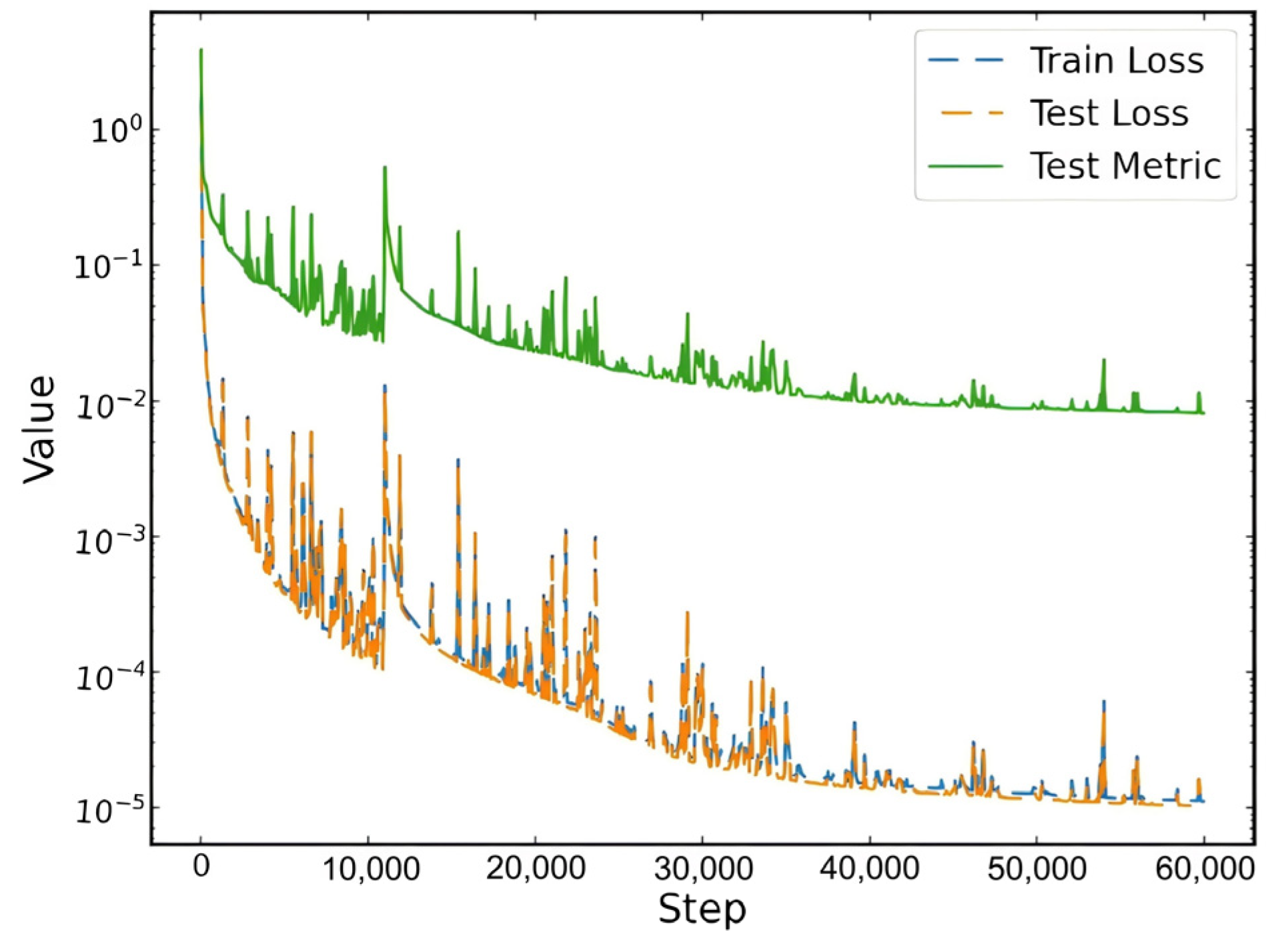
The training and testing comprise a training set of 1000 samples and a test set of 200 samples. As illustrated in Figure 21 the training losses for displacement field converge effectively on both the training and test sets of BC1. This convergence indicates that the GS-PI-DeepONets model is capable of extracting key physical information from geometric topology (via node coordinates), load characterization, and mechanical connectivity (via edge indices). Notably, the model demonstrates strong generalization capabilities, allowing for accurate predictions of mechanical field distributions under a variety of parametric conditions.

The performance of various methods on the test set is summarized in

Table 6. Performance comparison of different methods in static analysis of the support bracket of case 2 with BC1.

Predicted Field	Metric	FEM	PI-DeepGraphONets	DeepONets
Displacement Field	Mean R2	/	0.9999	0.9848
Displacement Field	Mean Relative $L_2$ Error	/	0.0086	0.0771
Data Generation Time (s)	Data Generation Time (s)	/	2522.8	2522.8
Training Time (s)	Training Time (s)	/	752.0	847.2
Solving Time (s)	Solving Time (s)	2.0209	0.2653	0.2721

. The suggested method achieves an R² of 0.9999 with a relative error of $8.60\times {10}^{-3}$, indicating an excellent agreement between the predicted and reference solutions. For the stress field, the method achieves an R² of 0.9991 with a relative error of $2.15\times {10}^{-2}$. Notably, the operator-learning approach performs better for displacement than for stress, as the stress field relies on spatial derivatives of displacement, (which involve complex calculations through the strain-displacement matrix, the Jacobian matrix, and constitutive equations.

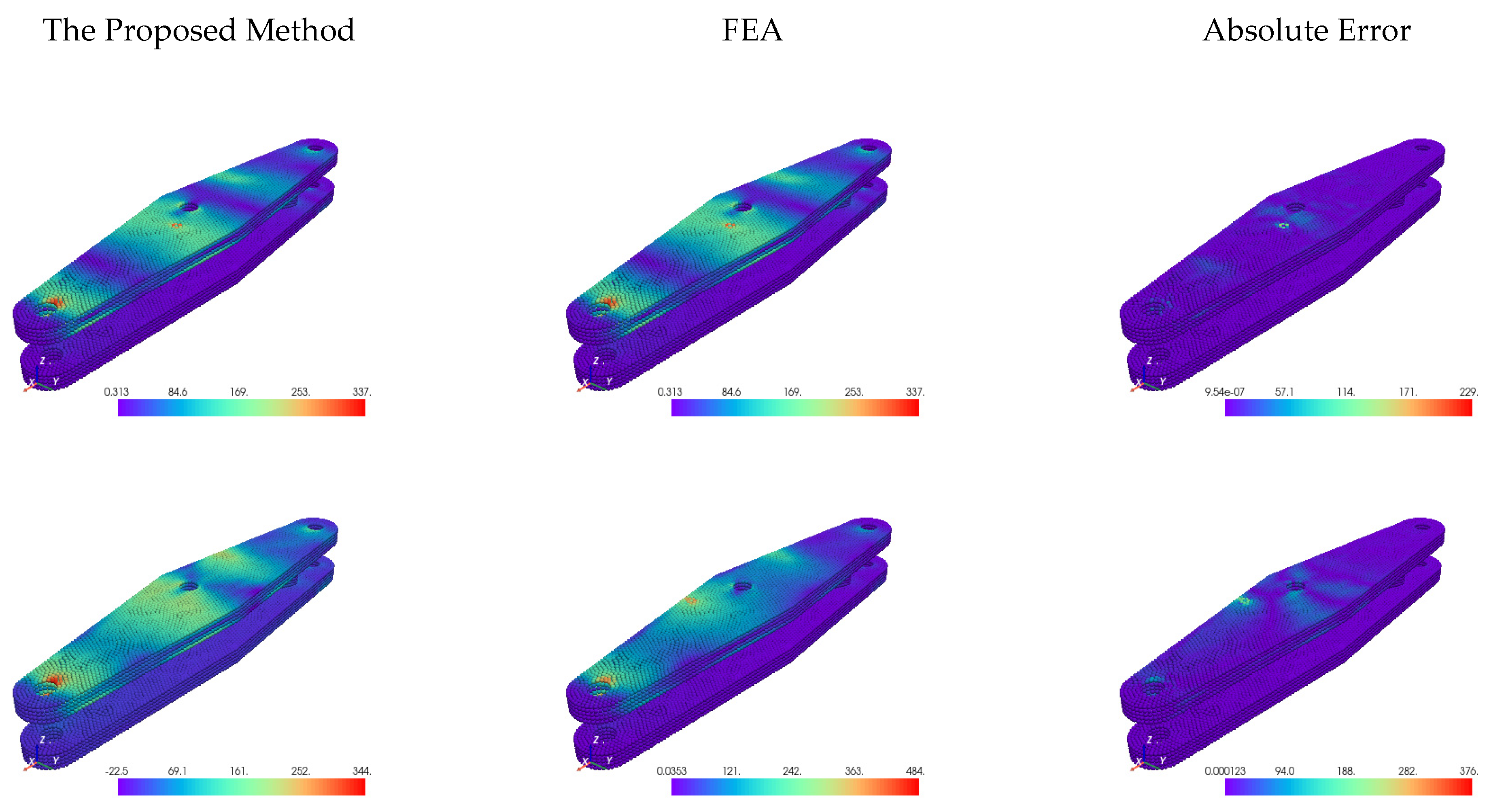
The comparative results of the GS-PI-DeepONets predictions against the FEM reference solutions for displacement distribution are presented. In these Figure 22, a consistent layout is adopted: predictions made by GS-PI-DeepONets are displayed on the left, with FEM reference solutions for comparison in the middle, and the absolute errors between the two on the right. From top to bottom, the cases shown correspond to the maximum, median, and minimum relative errors in the test set, providing a comprehensive view of the performance across different error ranges. The error distributions for both displacement and stress fields are visualized for both in-domain and out-of-domain test cases, as shown. Furthermore, it should be noted that displacement errors propagate to stress errors due to gradient amplification during backpropagation. Consequently, stress errors are larger in magnitude but follow a similar distribution pattern as displacement errors.

To further investigate the suggested method, the results of case 2 with BC2 are also demonstrated. For the BC2, as shown in Figure 23, both training and test losses exhibit smooth and stable convergence. The close alignment between training and test losses indicates excellent generalization performance with no over-fitting. Moreover, the simulation results are illustrated in Figure 24 and corresponding criteria for efficiency and accuracy are listed in

Table 7. Performance comparison of different methods in static analysis of the support bracket of case 2 with BC2.

Predicted Field	Metric	FEM	PI-DeepGraphONets	DeepONets
Displacement Field	Mean R2	/	0.9999	0.9848
Displacement Field	Mean Relative $L_2$ Error	/	0.0001	0.0771
Data Generation Time (s)	Data Generation Time (s)	/	2443.7	2623.1
Training Time (s)	Training Time (s)	/	753.0	806.4
Solving Time (s)	Inference Time (s)	2.0209	0.2341	0.2687

. Obviously, the proposed GS-PI-DeepONets method demonstrates significant improvements in both accuracy and training efficiency.

7.3. Summaries

The two case studies illustrate that GS-PI-DeepONets consistently outperforms both traditional FEM and the original DeepONets across structural problems resembling shells and solids. For the reclining adjuster connector (a shell model with 2126 S4R elements), the algorithm achieves a mean R² of 0.9832 and a relative $L_2$ error of $6.85\times {10}^{-2}$, surpassing DeepONets (0.9548, 0.1240) while reducing inference time from 2.0163 s (FEM) to 0.2601 s. For the support arm (a solid C3D8R model with 5594 elements), it achieves even greater accuracy—0.9999 R² and an 8.6 × 10⁻³ error for displacement, 0.9991 R² and a $2.15\times {10}^{-2}$ error for von-Mises stress—again improving on DeepONets (0.9848/0.9734 R², 0.0771/0.0946 error) and decreasing solve time from 2.0209 s (FEM) to approximately 0.266 s. Training remains efficient (314–752 s compared to 349–851 s for DeepONets), and the initial data-generation cost (2522.8 s) is amortized over thousands of rapid queries. Error distributions remain compact within the sampled load domain and are acceptable outside it, confirming strong generalization capabilities. Overall, GS-PI-DeepONets delivers FEM-grade fidelity with a 7–8 speed-up and significantly better accuracy than previous operator-learning baselines, making it an effective real-time surrogate for predicting both displacement and stress in complex automotive structures.

8. Conclusions

This study introduces the GS-PI-DeepONet, a novel neural framework designed to address the challenges of solving parametric PDEs in structural analysis, particularly for problems involving complex geometries and dynamic boundary conditions. By integrating GNNs, DeepONets and PINNs, the proposed method achieves significant improvements in accuracy, efficiency, and generalization compared to traditional numerical solvers and existing data-driven approaches.

The GS-PI-DeepONet leverages graph-structured data to model unstructured FE meshes and point clouds, efficiently capturing geometric and topological relationships. Nodes within this framework encode physical quantities such as displacements and loads, while edges represent connectivity or coupling, enabling the model to handle complex geometries and multi-scale features seamlessly. By embedding PDE constraints directly into the loss function, the model ensures that predictions adhere to the underlying physical laws, reducing the reliance on large datasets and enhancing generalization, particularly in scenarios with sparse or noisy data. Furthermore, the framework extends DeepONets to graph-structured inputs, enabling resolution-independent predictions and efficient handling of parametric PDEs. The branch and trunk networks map boundary conditions and spatial coordinates into a shared latent space, facilitating rapid inference for new parameter instances without re-simulation.

Extensive experiments on benchmark and real-world engineering problems have demonstrated the superiority of GS-PI-DeepONet. For instance, in the simply supported beam benchmark, the model achieves an $R^2$ value of 0.9999 and $L_2$ error of 5.45 × 10⁻² for in-distribution predictions, with comparable performance for out-of-distribution samples. In real-world applications, such as recliner mechanism stiffness analysis and support bracket strength analysis, the model outperforms traditional FEM and vanilla DeepONets, achieving speed-ups of 7–8 times while maintaining high accuracy. $R^2=0.9991$ Additionally, the model exhibits strong generalization capabilities, as evidenced by its compact error distributions and rare anomalies, confirming its ability to handle diverse and unseen scenarios.

Generally, the GS-PI-DeepONet offers a practical alternative to the traditional FEM for real-time simulations, particularly in applications requiring rapid parameter sweeps or design optimizations, such as in automotive or aerospace engineering. This method substantially alleviates the computational load associated with high-fidelity simulations by distributing the initial data-generation cost over thousands of queries, thereby reducing computational costs. Additionally, the framework is flexible and can be applied to a variety of structural problems, encompassing shell and solid mechanics. Its versatility extends to other fields involving parametric PDEs, including fluid dynamics and heat transfer, making it a highly adaptable tool with broad application potential.

Despite its advantages, the GS-PI-DeepONet framework has certain limitations. Like most data-driven approaches, it relies on a pre-generated dataset—typically obtained from high-fidelity FEM simulations—for training. While the model significantly reduces the need for large datasets through physics-informed regularization, the initial data generation process remains computationally expensive. Additionally, the current implementation is best suited for static linear-elastic problems; extending it to dynamic, nonlinear, or multiphysics scenarios would require further architectural and theoretical developments. Future work will focus on reducing data dependency through transfer learning and few-shot learning techniques, as well as extending the model to time-dependent and material-nonlinear problems.

References

1. Han, J.; Jentzen, A.; Weinan, E. Solving high-dimensional partial differential equations using deep learning. Proc. Natl. Acad. Sci. USA 2018, 115, 8505–8510. [Google Scholar] [CrossRef] [PubMed]
2. Raissi, M.; Perdikaris, P.; Karniadakis, G.E. Physics-informed neural networks: A deep learning framework for solving forward and inverse problems involving nonlinear partial differential equations. J. Comput. Phys. 2019, 378, 686–707. [Google Scholar] [CrossRef]
3. Cheng, M.; Fang, F.; Pain, C.C.; Navon, I.M. Data-driven modelling of nonlinear spatio-temporal fluid flows using a deep convolutional generative adversarial network. Comput. Methods Appl. Mech. Eng. 2020, 365, 113000. [Google Scholar] [CrossRef]
4. Jiang, X.; Wang, X.; Wen, Z.; Wang, H. Resolution-independent generative models based on operator learning for physics-constrained Bayesian inverse problems. Comput. Methods Appl. Mech. Eng. 2024, 420, 116690. [Google Scholar] [CrossRef]
5. Haghighat, E.; Raissi, M.; Moure, A.; Gomez, H. A physics-informed deep learning framework for inversion and surrogate modeling in solid mechanics. Comput. Methods Appl. Mech. Eng. 2021, 379, 113741. [Google Scholar] [CrossRef]
6. Wen, Z.; Li, Y.; Wang, H.; Peng, Y. Data-driven spatiotemporal modeling for structural dynamics on irregular domains by stochastic dependency neural estimation. Comput. Methods Appl. Mech. Eng. 2023, 404, 115831. [Google Scholar] [CrossRef]
7. Cai, S.; Mao, Z.; Wang, Z.; Yin, M.; Karniadakis, G.E. Physics-informed neural networks (PINNs) for fluid mechanics: A review. Acta Mech. Sin. 2021, 37, 1727–1738. [Google Scholar] [CrossRef]
8. He, W.; Li, J.; Kong, X.; Xu, Y. Multi-level physics informed deep learning for solving partial differential equations in computational structural mechanics. Commun. Eng. 2024, 3, 151. [Google Scholar] [CrossRef]
9. Wang, S.; Sankaran, S.; Perdikaris, P. Adaptive activation functions for scalable PINN architectures. Comput. Methods Appl. Mech. Eng. 2023, 407, 115887. [Google Scholar]
10. De Ryck, T.; Mishra, S.; Molinaro, R. wPINNs: Weak physics informed neural networks for approximating entropy solutions of hyperbolic conservation laws. SIAM J. Numer. Anal. 2024, 62, 811–841. [Google Scholar] [CrossRef]
11. Lu, L.; Pestourie, R.; Yao, W.; Wang, Z.; Verdugo, F.; Johnson, S.G. Physics-informed neural networks with hard constraints for inverse design. SIAM J. Sci. Comput. 2021, 43, B1105–B1132. [Google Scholar] [CrossRef]
12. Yin, J.; Wen, Z.; Li, S.; Zhang, Y.; Wang, H. Dynamically configured physics-informed neural network in topology optimization applications. Comput. Methods Appl. Mech. Eng. 2024, 426, 117004. [Google Scholar] [CrossRef]
13. Dwivedi, V.; Parashar, N.; Srinivasan, B. Distributed physics informed neural network for data-efficient solution to partial differential equations. Neurocomputing 2021, 420, 299–316. [Google Scholar] [CrossRef]
14. Luo, K.; Zhao, J.; Wang, Y.; Li, J.; Wen, J.; Liang, J.; Soekmadji, H.; Liao, S. Physics-informed neural networks for PDE problems: A comprehensive review. Artif. Intell. Rev. 2025, 58, 323. [Google Scholar] [CrossRef]
15. Simo, J.C.; Armero, F.; Taylor, C.A. Stable and time-dissipative finite element methods for the incompressible Navier–Stokes equations in advection dominated flows. Int. J. Numer. Methods Eng. 1995, 38, 1475–1506. [Google Scholar] [CrossRef]
16. Nooraiepour, M. Traditional and Machine Learning Approaches to Partial Differential Equations: A Critical Review of Methods, Trade-Offs, and Integration. Preprints 2025, 2025090472. [Google Scholar]
17. Difonzo, F.V.; Lopez, L.; Pellegrino, S.F. Physics informed neural networks for an inverse problem in peridynamic models. Eng. Comput. 2024, in press. [Google Scholar] [CrossRef]
18. Yang, L.; Perdikaris, P. Adversarial uncertainty quantification in physics-informed neural networks. J. Comput. Phys. 2023, 394, 136–152. [Google Scholar] [CrossRef]
19. Jiang, X.; Wang, X.; Wen, Z.; Li, E.; Wang, H. Practical uncertainty quantification for space-dependent inverse heat conduction problem via ensemble physics-informed neural networks. Int. Commun. Heat Mass Transf. 2023, 147, 106940. [Google Scholar] [CrossRef]
20. Wang, X.; Jiang, X.; Wang, H.; Li, G. Manifold learning-assisted uncertainty quantification of system parameters in the fiber metal laminates hot forming process. J. Intell. Manuf. 2025, 36, 2193–2219. [Google Scholar] [CrossRef]
21. Wang, H.; Zhou, W.; Wang, H.; Li, G. A DeepONets-based resolution independent ABC inverse method for determining material parameters of HAZ. Eng. Fract. Mech. 2025, 315, 110843. [Google Scholar] [CrossRef]
22. Long, Z.; Lu, Y.; Ma, X.; Dong, B. PDE-Net: Learning PDEs from data. In Proceedings of the 35th International Conference on Machine Learning, Stockholm, Sweden, 10–15 July 2018; Dy, J., Krause, A., Eds.; PMLR: Stockholm, Sweden, 2018; pp. 3208–3216. [Google Scholar]
23. Lu, L.; Jin, P.; Pang, G.; Zhang, Z.; Karniadakis, G.E. Learning nonlinear operators via DeepONet based on the universal approximation theorem of operators. Nat. Mach. Intell. 2021, 3, 218–229. [Google Scholar] [CrossRef]
24. Hao, Z.; Liu, S.; Zhang, Y.; Ying, C.; Feng, Y.; Su, H.; Zhu, J. GNOT: A general neural operator transformer for operator learning. In Proceedings of the 40th International Conference on Machine Learning (ICML), Honolulu, HI, USA, 23–29 July 2023. [Google Scholar]
25. Tran, A.; Mathews, A.; Xie, L.; Ong, C.S. Factorized Fourier Neural Operators for PDEs. In Proceedings of the 40th International Conference on Machine Learning (ICML), Honolulu, HI, USA, 23–29 July 2023. [Google Scholar]
26. Goswami, S.; Kontolati, K.; Shields, M.D.; Karniadakis, G.E. Deep transfer operator learning for partial differential equations under conditional shift. Nat. Mach. Intell. 2022, 4, 1155–1164. [Google Scholar] [CrossRef]
27. Li, J.; Liu, W. An approximate operator-based learning method for the numerical solutions of stochastic differential equations. arXiv 2023, arXiv:2312.08072. [Google Scholar] [CrossRef]
28. Yin, J.; Li, S.; Zhang, Y.; Wang, H. An efficient discrete physics-informed neural networks for geometrically nonlinear topology optimization. Comput. Methods Appl. Mech. Eng. 2025, 442, 118043. [Google Scholar] [CrossRef]
29. Zhang, E.; Yin, M.; Karniadakis, G.E. Physics-informed neural networks for nonhomogeneous material identification in elasticity imaging. arXiv 2020, arXiv:2009.04525. [Google Scholar] [CrossRef]
30. Lütjens, B.; Crawford, C.H.; Watson, C.D.; Hill, C.; Newman, D. Multiscale neural operator: Learning fast and grid-independent pde solvers. arXiv 2022, arXiv:2207.11417. [Google Scholar] [CrossRef]
31. Diab, A.; Abueidda, D.W.; Pantidis, P. DeepOKAN: Deep operator network based on Kolmogorov Arnold networks for mechanics problems. Comput. Methods Appl. Mech. Eng. 2025, 436, 117699. [Google Scholar] [CrossRef]
32. Sanchez-Gonzalez, A.; Godwin, J.; Pfaff, T.; Ying, R.; Leskovec, J.; Battaglia, P. Learning to simulate complex physics with graph networks. In Proceedings of the 37th International Conference on Machine Learning, Vienna, Austria, 13–18 July 2020; Daumé, H., III, Singh, A., Eds.; PMLR: Stockholm, Sweden, 2020; pp. 8459–8468. [Google Scholar]
33. Pfaff, T.; Fortunato, M.; Sanchez-Gonzalez, A.; Battaglia, P. Learning mesh-based simulation with graph networks. In Proceedings of the International Conference on Learning Representations, Addis Ababa, Ethiopia, 26–30 April 2020. [Google Scholar]
34. Brandstetter, J.; Berg, R.v.d.; Welling, M.; Gupta, J.K. Geometric and Physical Quantities Improve E(3) Equivariant Message Passing. In Proceedings of the International Conference on Learning Representations (ICLR), Virtual Event, 25–29 April 2022. [Google Scholar]
35. Li, Z.; Huang, D.Z.; Lin, G. E(n)-Equivariant Graph Neural Networks for PDEs on Dynamic Geometries. J. Mach. Learn. Res. 2024, 25, 1–35. [Google Scholar]
36. Wang, R.; Walters, R.; Yu, R. Equivariant Graph Neural Networks for Learning PDEs on Deforming Meshes. In Proceedings of the 40th International Conference on Machine Learning (ICML), Vienna, Austria, 21–27 July 2024. [Google Scholar]
37. Dwivedi, V.; Thandavan, A.; Srinivasan, B. Geometric Graph Learning for Computational Fluid Dynamics on Unstructured Meshes. Comput. Fluids 2024, 268, 106101. [Google Scholar]
38. Lino, M.; Cantwell, C.; Fotiadis, S.; Bharath, A.A.; Storkey, A. Simulating Continuum Mechanics with Multi-Scale Graph Neural Networks. Comput. Methods Appl. Mech. Eng. 2022, 390, 114474. [Google Scholar]
39. Bishnoi, S.; Bhattacharya, K.; Admal, P.C. GNN-based Physics Inference for Clerk-Maxwell’s Equations. J. Comput. Phys. 2023, 491, 112375. [Google Scholar]
40. Kashinath, K.; Mustafa, M.; Albert, A.; Wu, J.L.; Jiang, C.; Esmaeilzadeh, S.; Azizzadenesheli, K.; Anandkumar, A. MeshGraphNets 2.0: Towards Universal Physical System Simulators. arXiv 2025, arXiv:2502.01265. [Google Scholar]
41. Daw, A.; Karpatne, A.; Watkins, W.D.; Read, J.S. Physics-guided neural networks (PGNN): An application in lake temperature modeling. In Knowledge Guided Machine Learning; Karpatne, A., Majumdar, A.P., Kumar, V., Steinbach, M., Eds.; CRC Press: Boca Raton, FL, USA, 2022; pp. 353–376. [Google Scholar]
42. Faroughi, S.A.; Pawar, N.M.; Fernandes, C.; Raissi, M.; Das, S.; Kalantari, N.K.; Mahjour, S.K. Physics-guided, physics-informed, and physics-encoded neural networks and operators in scientific computing: Fluid and solid mechanics. J. Comput. Inf. Sci. Eng. 2024, 24, 040802. [Google Scholar] [CrossRef]
43. Kipf, T.N.; Welling, M. Semi-supervised classification with graph convolutional networks. arXiv 2017, arXiv:1609.02907. [Google Scholar] [CrossRef]
44. Jiang, B.; Zhang, Z.; Lin, D.; Tang, J.; Luo, B. Semi-supervised learning with graph learning-convolutional networks. In Proceedings of the IEEE/CVF Conference on Computer Vision and Pattern Recognition, Long Beach, CA, USA, 15–20 June 2019; pp. 11305–11312. [Google Scholar]
Figure 1. An illustration of simply supported beam problem.
Make 07 00137 g001
Figure 2. An illustration of GATs.
Make 07 00137 g002
Figure 3. An illustration of the geometric embedding of DeepONet.
Make 07 00137 g003
Figure 4. An illustration of the GS-PI-DeepONet architecture.
Make 07 00137 g004
Figure 5. Training process of the GS-PI-DeepONets model for cantilever beam.
Make 07 00137 g005
Figure 6. Comparison of the deflection of the top surface by the simulation matches the analytical solution for a cantilever beam.
Make 07 00137 g006
Figure 7. Predicated Von Mises stress (left) and displacement magnitude (right) of cantilever beam.
Make 07 00137 g007
Figure 8. An illustration of the Hertz problem.
Make 07 00137 g008
Figure 9. Training process of the GS-PI-DeepONets model for Hertz problem.
Make 07 00137 g009
Figure 10. The predicted Von Mises stress (left) and displacement magnitude (right) for the Hertz problem.
Make 07 00137 g010
Figure 11. Comparison between the predicted contact pressure distribution and the Hertz theory.
Make 07 00137 g011
Figure 12. The geometry of the connecting plate.
Make 07 00137 g012
Figure 13. The FE model along with the initial and boundary conditions for BC1.
Make 07 00137 g013
Figure 14. The FE model along with the initial and boundary conditions for BC2.
Make 07 00137 g014
Figure 15. Training process of the GS-PI-DeepONets model for case 1 with BC1.
Make 07 00137 g015
Figure 16. Comparison of the predicted, reference, and error distribution of displacement fields for case 1 with BC1 (Left: GS-PI-DeepONet; Middle: FEM; Right: Absolute Error).
Make 07 00137 g016
Figure 17. Training process of the GS-PI-DeepONets model for case 1 with BC2.
Make 07 00137 g017
Figure 18. Comparison of the predicted, reference, and error distribution of displacement fields for case 1 with BC2 (Left: GS-PI-DeepONet; Middle: FEM; Right: Absolute Error).
Make 07 00137 g018
Figure 19. FE model and boundary conditions of the support bracket with BC1.
Make 07 00137 g019
Figure 20. FE model and boundary conditions of the support bracket with BC2.
Make 07 00137 g020
Figure 21. Training loss convergence curves for displacement field predictions of case 2 with BC1.
Make 07 00137 g021
Figure 22. Predicted vs. reference displacement responses for case 2 with BC1 (Left: GS-PI-DeepONet; Middle: FEM; Right: Absolute Error).
Make 07 00137 g022
Figure 23. Training loss convergence curves for displacement field predictions of case 2 with BC2.
Make 07 00137 g023
Figure 24. Comparison of the predicted, reference, and error distribution of displacement fields for case 2 with BC2 (Left: GS-PI-DeepONet; Middle: FEM; Right: Absolute Error).
Make 07 00137 g024