Article

A Novel Spatio-Temporal Graph Convolutional Network with Attention Mechanism for PM2.5 Concentration Prediction

School of Cyberspace Security (School of Cryptology), Hainan University, Haikou 570228, China
*
Authors to whom correspondence should be addressed.
These authors contributed equally to this work.
Mach. Learn. Knowl. Extr. 2025, 7(3), 88; https://doi.org/10.3390/make7030088
Submission received: 17 June 2025 / Revised: 3 August 2025 / Accepted: 25 August 2025 / Published: 27 August 2025

Abstract

Accurate and high-resolution spatio-temporal prediction of PM2.5 concentrations remains a significant challenge for air pollution early warning and prevention. Advanced artificial intelligence (AI) technologies, however, offer promising solutions to this problem. A spatio-temporal prediction model is designed in this study, which is built upon a seq2seq architecture. This model employs an improved graph convolutional neural network to capture spatially dependent features, integrates time-series information through a gated recurrent unit, and incorporates an attention mechanism to achieve PM2.5 concentration prediction. Benefiting from high-resolution satellite remote sensing data, the regional, multi-step and high-resolution prediction of PM2.5 concentration in Beijing has been performed. To validate the model’s performance, ablation experiments are conducted, and the model is compared with other advanced prediction models. The experimental results show our proposed Spatio-Temporal Graph Convolutional Network with Attention Mechanism (STGCA) outperforms comparison models in multi-step forecasting, achieving root mean squared error (RMSE), mean absolute error (MAE) and mean absolute percentage error (MAPE) of 4.21, 3.11 and 11.41% for the first step, respectively. For subsequent steps, the model also shows significant improvements. For subsequent steps, the model also shows significant improvements, with RMSE, MAE and MAPE values of 5.08, 3.69 and 13.34% for the second step and 6.54, 4.61 and 16.62% for the third step, respectively. Additionally, STGCA achieves the index of agreement (IA) values of 0.98, 0.97 and 0.95, as well as Theil’s inequality coefficient (TIC) values of 0.06, 0.08 and 0.10 proving its superiority. These results demonstrate that the proposed model offers an efficient technical approach for smart air pollution forecasting and warning in the future.

1. Introduction

With the acceleration of urbanization, air pollution has become a critical environmental issue in cities worldwide. Among the various pollutants, fine particulate matter with a diameter of 2.5 microns or less PM2.5 is of primary concern due to its severe health implications. These microscopic particles can penetrate deep into the human respiratory system, leading to a range of cardiovascular and respiratory diseases and an increased risk of premature mortality [1]. Beyond its impact on human health, high concentrations of PM2.5 also contribute to broader environmental issues, including ecosystem degradation [2]. Therefore, accurately predicting PM2.5 concentration to support decision makers in air quality management is of great practical value and scientific significance.
Although ground-based monitoring stations can provide information on pollutant concentration in some areas, their coverage is limited, and it is difficult to meet the demand for high resolution in time and space. In recent years, the development of satellite remote sensing technology has brought new opportunities for air quality monitoring. Remote sensing data including Aerosol Optical Thickness (AOD), meteorological data, and the Normalized Vegetation Index (NDVI), provide more dimensional information for PM2.5 prediction. However, the task of PM2.5 prediction still faces challenges, especially in effectively integrating multi-source data and capturing their complex spatial and temporal dependencies.
The existing approaches to forecast the concentrations of air pollutants can be roughly divided into three categories, namely numerical forecast, statistical forecast and artificial intelligence (AI). Numerical models are designed to replicate the physical, chemical, and transport processes of pollutants in the atmosphere by solving intricate differential equations. Notable examples of such models include the Community Multi-Scale Air Quality (CMAQ) [3] and the Weather Research and Forecasting model coupled with Chemistry (WRF-Chem) [4]. The performance of these models largely depends on accurate emission data for pollutant sources, which are often uncertain or unavailable. Additionally, the modeling process is computationally intensive and time-consuming. Thus, there is a need for the development of more efficient and precise models to improve air quality forecasting.
In contrast, statistical models are based on data mining of the internal relationships within historical data related to pollution. Classic examples, such as the Autoregressive Integrated Moving Average (ARIMA) model [5], are relatively simple to implement, and approaches like Multiple Linear Regression (MLR) have also been applied with success for pollutant forecasting [6]. However, these models are more suitable for smaller datasets and univariate time series analysis. Moreover, these models are based on linear assumptions and have strict requirements on the stationarity of the data. Hence, it is inherently difficult to capture the nonlinear relationships within data. These restrictions greatly limit the performance and applicability of classical statistical models in air pollution prediction.
Compared to conventional statistical models, AI models can approximate complex nonlinear relationships and tend to have stronger robustness and fault tolerance [7,8]. To address the challenge of nonlinearity, various machine learning (ML) algorithms have been widely adopted for air pollution forecasting. Models such as Support Vector Regression (SVR) [9], Random Forest (RF) [10], Extreme Gradient Boosting (XGB) [11], and Artificial Neural Networks (ANN) [12] have demonstrated their capability in this domain. For example, one study by Li et al. [13] successfully developed a hybrid system combining a least squares support vector machine (LSSVM) with a multi-objective optimization algorithm to forecast the Air Quality Index (AQI), validating its effectiveness across multiple cities.
However, traditional machine learning models usually require researchers to manually construct features, which is heavily dependent on personal experience. Moreover, they exhibit insufficient ability to reduce redundant data, which in turn affects their learning and generalization abilities when processing increasingly large datasets [14].
Recently, deep learning algorithms have made major breakthroughs in various areas such as computer vision, emotion recognition, and machine translation. As the latest AI achievement, deep learning algorithms have also become a hotspot in the field of air pollution prediction for their powerful feature learning and nonlinear mapping capabilities [15]. Among the various architectures, Recurrent Neural Networks (RNNs) and their variants—such as Long Short-Term Memory (LSTM) and Gated Recurrent Units (GRU)—are widely used for sequence prediction [16], while Transformer-based models, which first achieved state-of-the-art performance in Natural Language Processing (NLP), have since been successfully applied in many domains. RNNs remain a powerful and prevalent choice for spatio-temporal forecasting. This is often attributed to their inherent recurrent structure, which provides a strong inductive bias for ordered time-series data, and their linear complexity with respect to sequence length, which can be more efficient than the quadratic complexity of standard Transformers [17]. These models not only depend on information obtained at the current point in time but also consider prior information from previous moments. This characteristic is highly suitable for time-series air pollution prediction, making RNN-based models a mainstream approach in this field.
Given their ability to capture time dependencies in sequence data, RNN-based models are generally preferred over other statistical and machine learning models. However, air pollution prediction requires modeling the spatio-temporal relationships among various non-stationary air pollutant data and meteorological data [18]. Single RNN-based models may still be inadequate in dealing with the complex spatio-temporal dependencies. To overcome the drawbacks of single RNN models, researchers have explored other deep learning algorithms to enhance spatio-temporal modeling. Convolutional Neural Networks (CNNs) have been widely used due to their outstanding feature extraction capabilities, stemming from weight sharing and local awareness through the convolutional operation [19]. For example, Sayeed et al. [20] adopted a CNN model to forecast O3 concentration 24 h ahead. The model incorporated both air pollution and meteorology data, and the results showed that the CNN model outperformed traditional methods like Ridge and Lasso regression. Mo et al. [21] proposed TSTM, an integrated CNN-BiLSTM-Attention model with ConvLSTM enhancement, for multistep prediction of hourly concentrations of six conventional air pollutants in regional air quality forecasting, demonstrating superior prediction accuracy. In order to more effectively model complex spatio-temporal dependencies, especially the complex interactions between pollutants and meteorological factors, researchers have begun to explore more advanced models, such as Graph Convolutional Networks (GCN). GCN, with its ability to process graph-structured data, can better capture spatial dependencies and provide new solutions for air pollution prediction. GCNs are particularly effective in capturing complex spatial dependencies, making them well-suited for predicting the concentrations of air pollutants; while Euclidean distance accurately measures the physical proximity between monitoring stations, it is often insufficient for capturing the full complexity of pollution dynamics, which are influenced by factors beyond simple distance. For example, two stations may be geographically close but separated by a mountain, limiting direct pollutant transport. Conversely, two distant stations aligned with prevailing wind patterns may exhibit strong correlations. Graph-based representations are uniquely suited to model such connections, where edges can represent these complex dependencies. GCNs can then learn from this rich relational structure, leading to more accurate predictions. Several studies have explored the combination of GCN and LSTMs, especially in the context of spatio-temporal forecasting. For example, Ehteram et al. [22] proposed a GCN-LSTM hybrid model for spatio-temporal prediction tasks, demonstrating that GCN’s ability to capture complex spatial relationships significantly improves the temporal prediction performance of LSTM models. Chen et al. [23] also combined GCN and LSTM to propose an air quality prediction model named AAMGCRN, demonstrating improved accuracy in predicting PM2.5, PM10, and O3 concentrations.
GRUs have demonstrated strong potential in modeling the complex spatial and temporal dependencies inherent in air pollution data. Unlike previous methods that either focus on spatial or temporal features alone, the combination of GCN and GRU can effectively capture non-Euclidean spatial correlations across grid points as well as temporal dynamics. GRUs, by employing a simplified gating mechanism with only reset and update gates, reduce model complexity and parameters compared to LSTMs, leading to faster training and reduced risk of overfitting. Motivated by these advantages, this study proposes a novel spatio-temporal model integrating GCN and GRU to improve PM2.5 concentration prediction. We further enhance the model with an attention mechanism to dynamically weigh spatial and temporal features, enabling the extraction of critical information from multi-source data.
The main innovations and contributions of this work are summarized as follows:
  • The Spatio-Temporal Graph Convolutional Network with Attention Mechanism (STGCA) model is proposed, which is designed based on a seq2seq framework, and is able to effectively capture the complex dependencies of PM2.5 concentration in both spatial and temporal dimensions by combining GCN and GRU. GCN processes the non-Euclidean spatial features for accurately modeling spatial correlations among different regions, while the GRU models time series information to capture the long-term and short-term temporal dynamics.
  • A spatio-temporal attention mechanism for air pollution prediction is designed, which is used to extract features in the temporal and spatial dimensions. By learning the distribution of attention weights, this mechanism can effectively extract important information to improve the prediction of air pollutant concentrations.
  • To objectively and comprehensively evaluate the proposed model, we design extensive experiments utilizing multi-source data, including air pollutant data, meteorological data and other relevant data. These experiments encompass multi-step regional prediction tasks of PM2.5 concentrations at high spatial resolution in Beijing and compare the model performance against baseline methods using various accuracy and robustness metrics.

2. Study Area and Dataset Analysis

2.1. Study Area

The study area covers the Beijing metropolitan region, a vital political, cultural, and economic center in China situated in the North China Plain. The selection of Beijing as the primary case study is motivated by its dual role as both a representative megacity and a region with unique and complex pollution dynamics. Specifically, its basin-like topography, surrounded by the Yan and Taihang Mountains, often traps local emissions, while its unique meteorological conditions facilitate the regional transport of pollutants from surrounding industrial zones. These factors, combined with elevated emissions from coal combustion for winter heating, create a challenging environment for air quality forecasting, making Beijing an ideal testbed for validating the performance and robustness of advanced spatio-temporal models. Concurrently, Beijing shares air quality challenges common to many rapidly urbanizing regions worldwide, including high population density and heavy vehicular traffic. Therefore, studying Beijing helps to address its own complex environmental problems. Furthermore, the methodology and conclusions from this research can provide a valuable reference for other cities facing similar challenges. This dual relevance justifies the selection of Beijing and underscores the value of this work.
The study area encompasses Beijing’s 16 administrative districts: Yanqing (YQ), Miyun (MY), Huairou (HR), Changping (CP), Pinggu (PG), Shunyi (SY), Haidian (HD), Chaoyang (CY), Tongzhou (TZ), Daxing (DX), Fangshan (FS), Mentougou (MTG), Shijingshan (SJS), Fengtai (FT), Dongcheng (DC), and Xicheng (XC). The map also shows the Beijing Capital International Airport, which is an administrative exclave of Chaoyang District. The overall study area is shown in Figure 1.

2.2. Dataset Description

In order to achieve high spatial and temporal resolution of predictions, remote sensing data with a resolution of 10 km is used for analysis and modeling of multiple raster cells for one city. Unlike data from monitoring stations, remote sensing data are characterized by wide coverage and high spatial resolution [24]. Data on air pollutant concentration, AOD, NDVI and meteorological factors are combined in this work to analyze the spatial and temporal distributions of PM2.5 concentrations and to make daily predictions.
Each grid point has its own time series, and the spatial distribution of PM2.5 concentration data from all grid points at a certain time can be abstracted into an undirected topological map. The spatial features at each time step are extracted to form a spatial feature time series, and then the time series based on the spatial feature timing dependence is decoded to obtain the target PM2.5 concentration.
The China High Resolution High Quality Near Surface Air Pollutants (CHAP) dataset served as the primary source for the experimental data in this study. This dataset is provided by the National Earth System Science Data Centre (NESDC) and is publicly accessible for download (https://www.aers-cloud.org.cn/) (accessed on 15 August 2024).
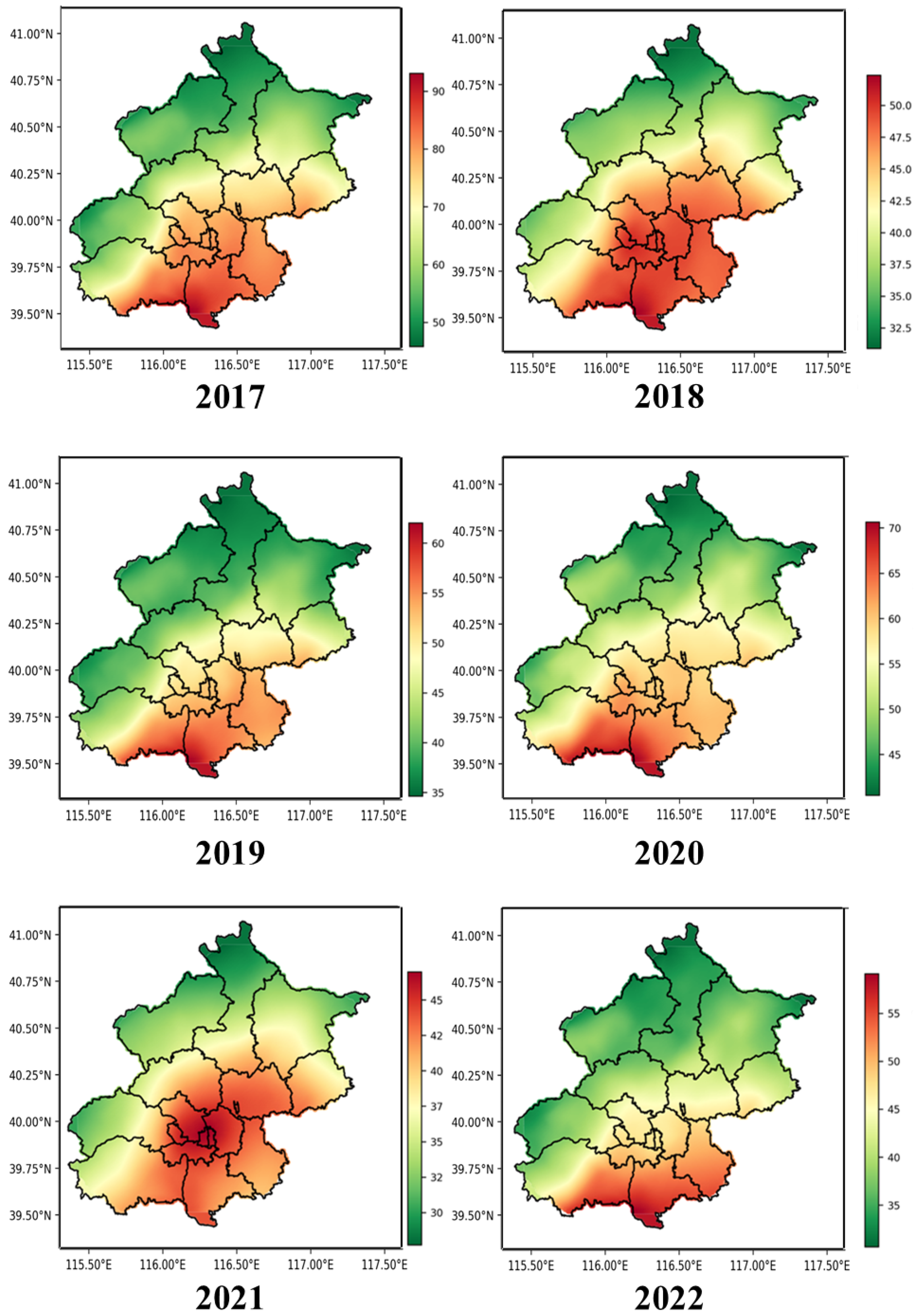
These datasets encompass six key air pollutants: PM2.5, PM10, NO2, CO, O3, and SO2 [25]. Figure 2 illustrates the spatial distribution of the annual average PM2.5 concentration across Beijing from 2017 to 2022. These maps enable an assessment of temporal trends in PM2.5 pollution, highlighting regions with persistently high concentrations as well as areas showing potential improvement. These co-pollutants are included as they are known precursors or indicators of atmospheric chemical processes that influence PM2.5 formation [26].
Meteorological data were derived from the ERA5-Land dataset, provided by the European Centre for Medium-Range Weather Forecasting (ECMWF) and accessible via the Copernicus Climate Data Store (https://cds.climate.copernicus.eu/) (accessed on 15 August 2024) [27]. This dataset was used to capture key atmospheric variables such as 2-m dewpoint temperature (D2m), 2-m temperature (T2m), total precipitation (TP), the 10-m u-component of wind (UW), the 10-m v-component of wind (VW), surface pressure (SP), and surface solar radiation (SSR). These factors critically modulate the dispersion, transformation, and deposition processes of PM2.5 and related pollutants. For the ERA5-Land hourly data, daily averages are calculated to align the temporal resolution with pollutant monitoring. These meteorological variables are crucial as they directly govern the transport, dispersion, and deposition of airborne particles [28].
Additionally, other data sources include AOD and NDVI data. The AOD data were also obtained from the National Earth System Science Data Centre (NESDC) [29], featuring a daily temporal resolution. This dataset provides critical information about the concentration and distribution of atmospheric aerosols, a key factor influencing PM2.5 pollution levels. The NDVI data are acquired from NASA’s Earth Observing System (NEO) platform, available at https://neo.gsfc.nasa.gov/ (accessed on 15 August 2024). To align with the daily frequency of our primary dataset, the monthly NDVI value was applied to each day within that respective month [30]. This dataset serves as a critical indicator of vegetation health and coverage. The NDVI directly influences atmospheric pollutant dynamics by mediating pollutant absorption and modifying local microclimatic conditions. Both AOD and NDVI have been widely demonstrated in previous studies to be significant predictors for ground-level PM2.5 concentrations [31,32].
To create a complete and robust spatio-temporal dataset, we employed a two-step hybrid interpolation strategy, similar to methods widely used in recent remote sensing studies [33]. First, a linear temporal interpolation was applied independently to each grid cell to fill short-term data gaps, effectively handling the majority of sporadic missing values. For any remaining gaps, a spatial interpolation based on the Inverse Distance Weighting (IDW) method was subsequently performed, imputing missing values by calculating a weighted average from the nearest neighboring cells at the same time step.
This dataset, with its extensive spatial and temporal coverage, provides a comprehensive foundation for atmospheric pollutant concentration prediction tasks, enabling detailed analysis of pollutant distributions and the influence of meteorological and environmental factors on air quality.
Table 1 details the experimental data and sources.
The data used in this study are publicly accessible and applicable to a broad range of regions. For instance, the CHAP dataset provides high-resolution pollutant data for many urban areas across China. Additionally, the ERA5-Land meteorological data and NASA NDVI products offer global coverage and are freely available. These characteristics ensure that the proposed model can be adapted not only to other cities within China but also to international regions with similar data availability.

2.3. Analysis of Temporal and Spatial Correlation

An analysis of the spatio-temporal characteristics of the PM2.5 concentration data was performed prior to model development. To this end, the stationarity of the time series was assessed using the Augmented Dickey–Fuller (ADF) test, while global spatial correlation analysis was employed to quantify the spatial relationships within the data. These preliminary statistical tests provide a scientific foundation for our predictive modeling approach.

2.3.1. Analysis of Temporal Correlation

The ADF test [34] was applied to evaluate the stationarity of the PM2.5 concentration time series. To obtain a single representative time series for the entire study area, the daily PM2.5 concentrations were spatially averaged across all 173 grid cells. The detailed results of the ADF test on this spatially averaged series are shown in Table 2.
The test statistic for the time series is −5.9135, which is much lower than the critical thresholds at the 1%, 5%, and 10% confidence levels. Additionally, the p-value is approximately 2.61 × 10 7 . These results strongly support the rejection of the null hypothesis, which posits the existence of a unit root. This confirms that the PM2.5 concentration time series is stationary over the studied period, ensuring its suitability for subsequent modeling.

2.3.2. Analysis of Spatial Correlation

PM2.5 concentrations are not only time-dependent but also exhibit significant spatial correlation. To evaluate this, this study utilizes Moran’s index to quantify both global and local spatial autocorrelation [35]. The Global Moran’s index (I) and the Local Moran’s index ( I i ) are defined as
I = N i = 1 N j = 1 N w i j i = 1 N j = 1 N w i j ( x i x ¯ ) ( x j x ¯ ) i = 1 N ( x i x ¯ ) 2
I i = x i x ¯ S 2 j = 1 N w i j ( x j x ¯ ) ,
where N is the number of spatial units, x i is the attribute value for unit i, x ¯ is the mean of the attribute, S 2 is the variance of the attribute, and w i j is the spatial weight between unit i and j.
A critical component of this analysis is the spatial weights matrix, W, which contains the weights w i j and defines the neighborhood relationships between locations. For the purpose of this exploratory spatial analysis, we constructed this matrix based on spatial contiguity using the K-Nearest Neighbors method. In this matrix, the weight w i j is set to 1 if location j is one of the 8 nearest neighbors of location i, and 0 otherwise. The resulting matrix was then row-standardized for the analysis [36].
Global Spatial Autocorrelation
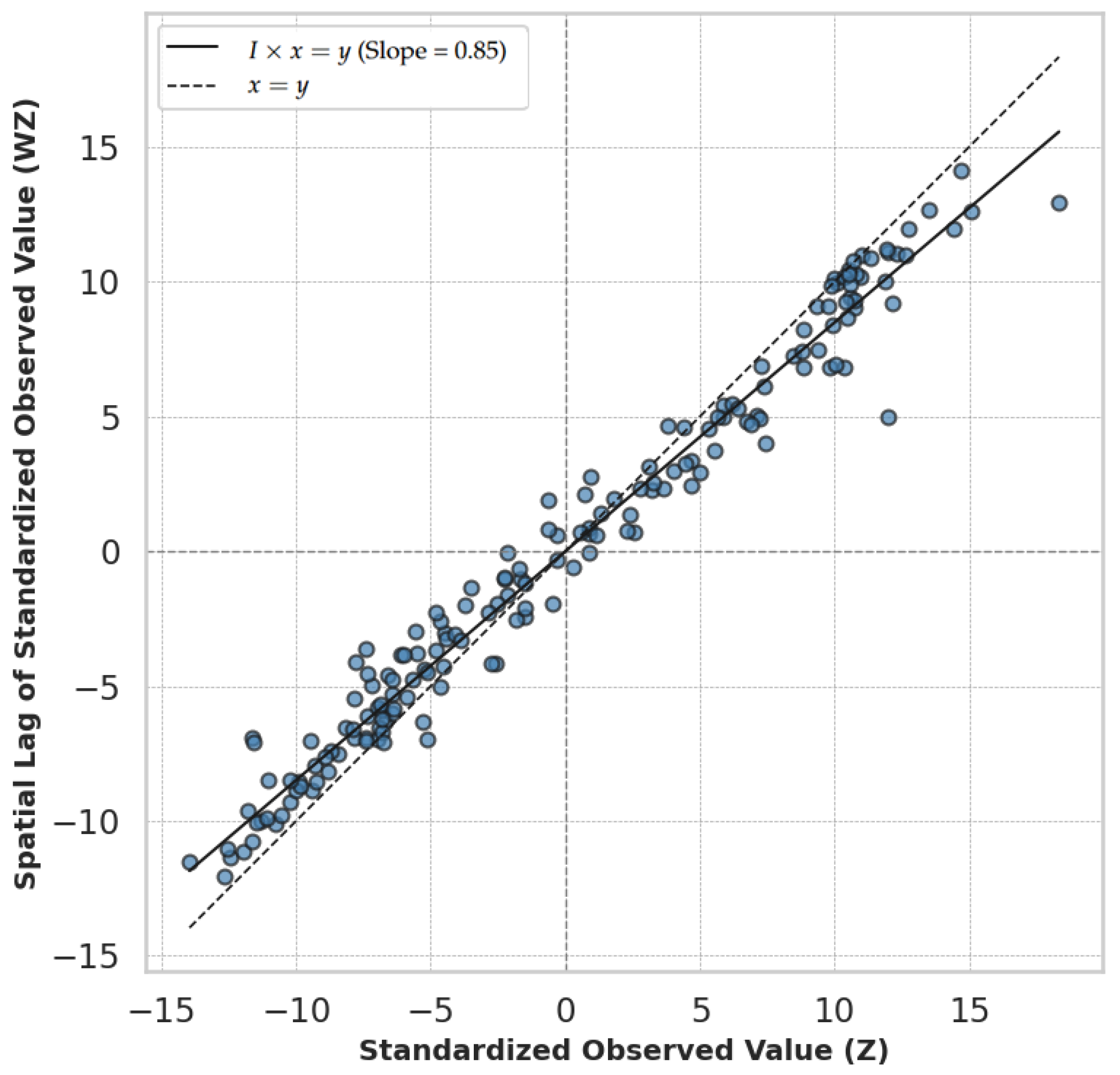
As shown in the scatter plot in Figure 3, the relationship between the standardized observed values (Z) and their spatial lags ( W Z ) demonstrates a clear positive linear trend. The regression line, representing I × x = y , has a slope of 0.85, which corresponds to the Global Moran’s I value. This positive trend, coupled with the concentration of points in the first (High-High) and third (Low-Low) quadrants, confirms that PM2.5 concentrations are not randomly distributed. Instead, they exhibit a significant spatial dependency where high-concentration areas tend to be located near other high-concentration areas, and vice versa.
Local Spatial Autocorrelation (LISA)
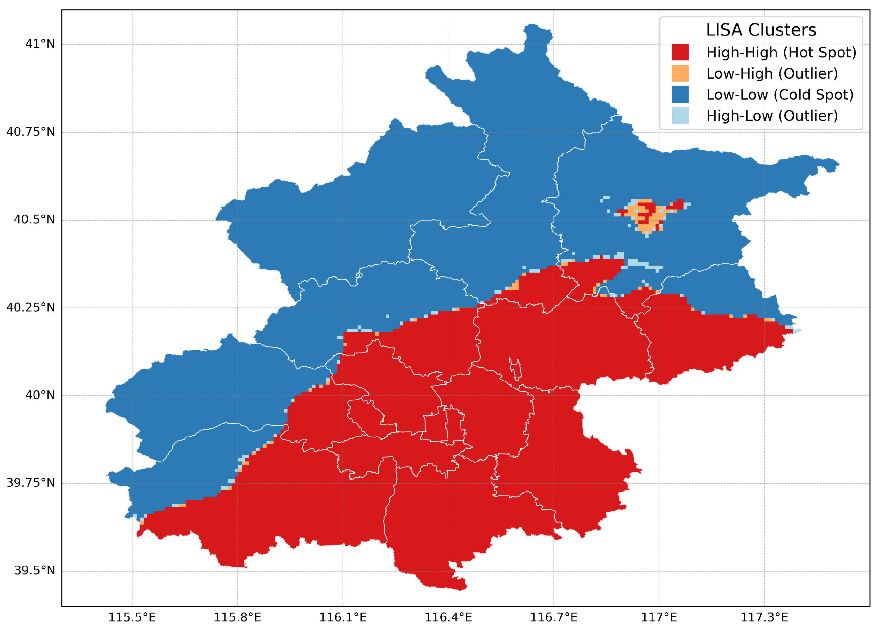
To identify the specific locations of statistically significant spatial clusters and outliers, we performed a Local Indicators of Spatial Association (LISA) analysis. The resulting cluster map is presented in Figure 4. The map reveals distinct spatial heterogeneity within Beijing. For instance, significant High-High clusters (hot spots) of PM2.5 concentration are predominantly located in the southern districts, which host more industrial and traffic activities. Conversely, Low-Low clusters (cold spots) are mainly found in the northern mountainous and suburban areas, such as Yanqing and Miyun. This analysis not only confirms the presence of localized clusters but also provides crucial spatial insights that justify the use of a graph-based model capable of capturing these specific local dependencies.

2.4. Evaluation Metrics

To thoroughly evaluate the model’s performance in predicting PM2.5 concentrations, a range of evaluation metrics is applied in this study. Specifically, root mean square error (RMSE), mean absolute error (MAE), and mean absolute percentage error (MAPE) are utilized to quantify the deviations and errors between the model’s predicted values and the observed data. Additionally, to further measure the relevance and accuracy of the model predictions, we use the index of agreement (IA) and Theil’s inconsistency coefficient (TIC) [37]. Smaller values of RMSE, MAE, MAPE, and TIC, as well as larger values of IA, indicate that the model has better predictive performance.
Table 3 summarizes all the evaluation metrics used for this comprehensive assessment.

3. Research Methodology

3.1. Prediction Model

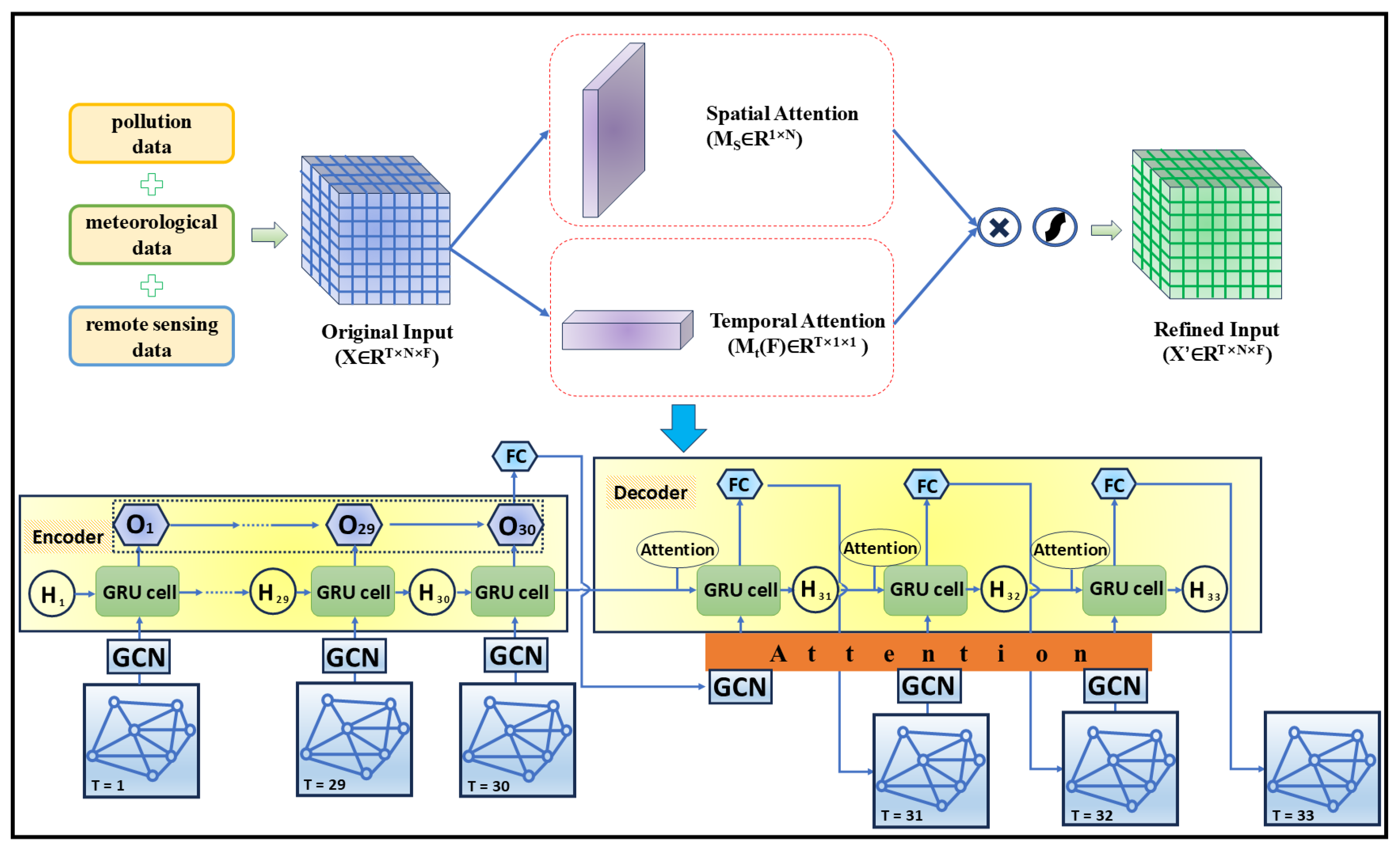
Figure 5 shows the process of our developed prediction method. It mainly consists of the following three steps:
  • We integrate and preprocess the multi-source data required for PM2.5 concentration prediction. These data include air pollutants, meteorological elements, and other environmental factors from remote sensing for Beijing. To effectively represent the spatio-temporal characteristics, the data for the 173 raster cells are structured into a tensor containing three dimensions: a temporal dimension representing the sequence of historical time steps, a spatial dimension corresponding to the raster cells, and a feature dimension. This results in a unified three-dimensional (3D) spatio-temporal matrix that provides high-precision input for the proposed model, ensuring that the model absorbs rich spatio-temporal information.
  • The spatio-temporal matrix is then processed by the attention module. This module contains two parts, spatial attention and temporal attention, which are used to assign spatial and temporal weights to the data.
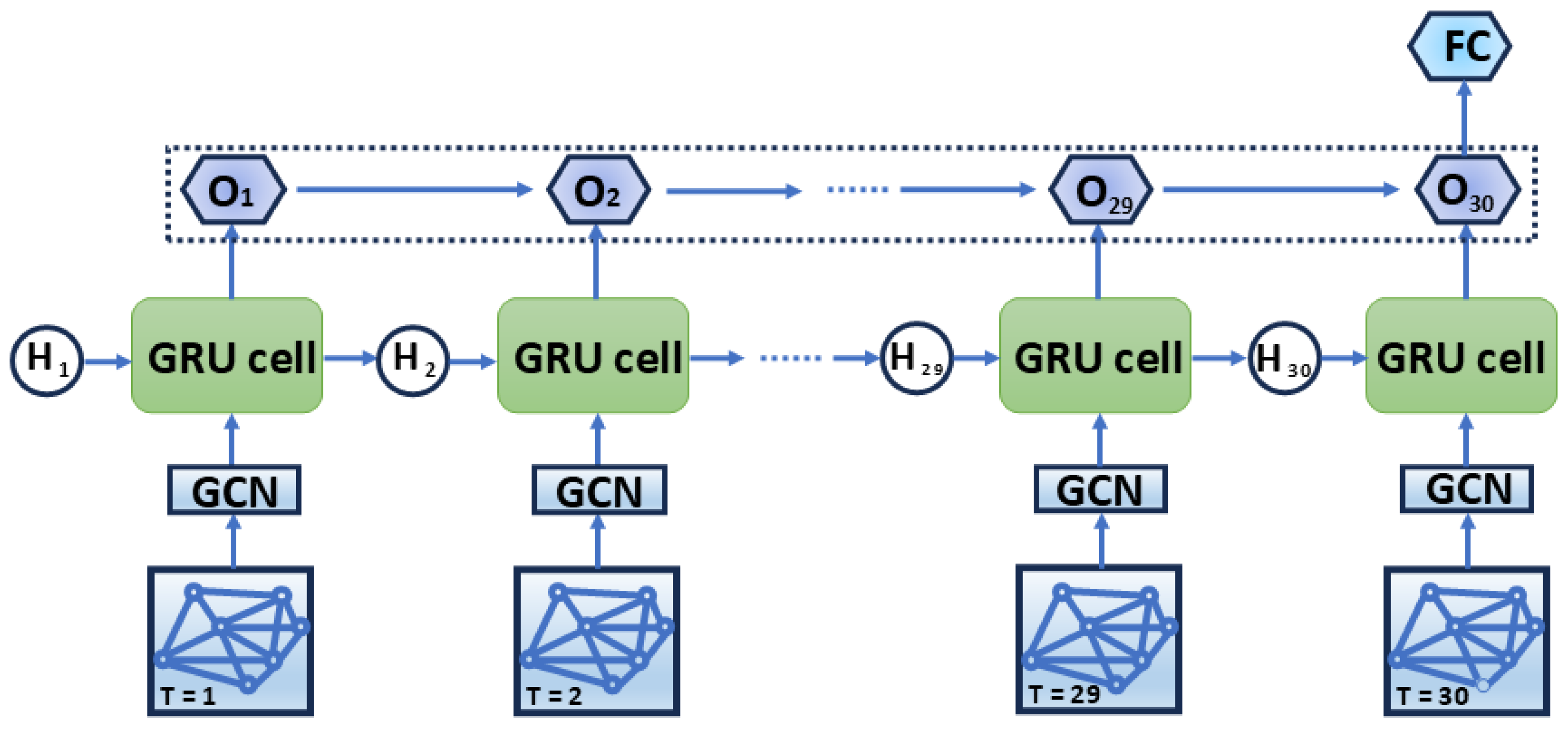
  • The refined input data are passed to the proposed STGCA prediction model. The model utilizes a seq2seq architecture that combines GCN and GRU. In the encoder, the GCN is tasked with modeling intricate spatial relationships among raster cells, while the GRU is used to process time-series information to capture dynamic patterns of PM2.5 concentrations over time. The hidden representation generated by the encoder is passed to the decoder, which realizes multi-step prediction through the GRU and GCN layers and enhances the time-dependent representation through the attention layer to generate PM2.5 concentration values at future moments. This structure effectively integrates the spatio-temporal features, which makes the model highly accurate in capturing the spatial and temporal dependence of PM2.5 concentration changes in the Beijing area [38].

3.2. Spatio-Temporal Attention Mechanism

The attention mechanism is inspired by the way humans focus on important information while ignoring irrelevant details. Its primary purpose is to identify intrinsic relationships in raw data, suppressing noise and emphasizing critical features through higher weights [39].
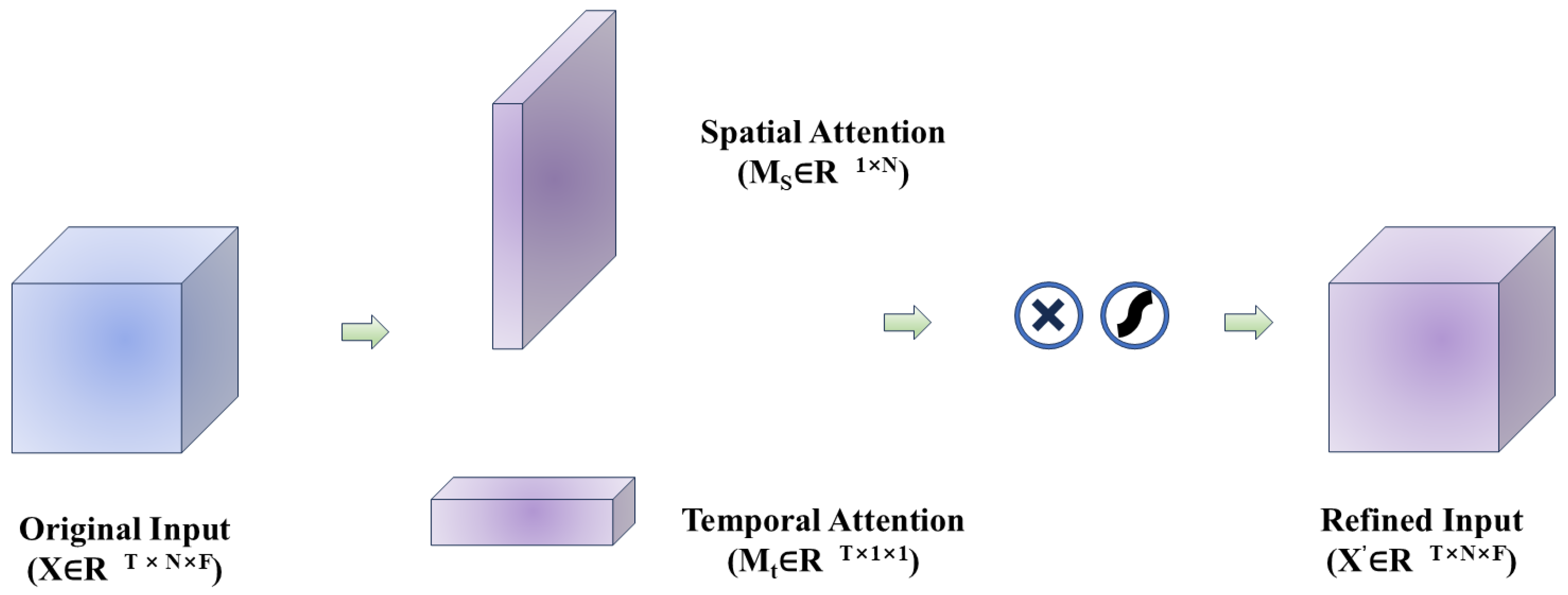
The input to the attention module is the three-dimensional tensor X R T × N × F , where T is the number of time steps, N is the number of spatial locations (raster cells), and F is the number of features. This clear tensor structure allows the subsequent attention modules to operate distinctly on the temporal (T) and spatial (N) axes.
Spatial attention (SA) and channel attention (CA) are extensively utilized in computer vision applications, demonstrating exceptional capabilities in allocating weights effectively across spatial and temporal dimensions to identify critical patterns [40].

3.2.1. Spatial Attention Module

The spatial attention module is designed to identify important spatial regions by analyzing inter-spatial relationships. As illustrated in Figure 6, this is achieved by first compressing the information across the temporal and feature dimensions (T and F axes). Specifically, both global max-pooling and global average-pooling operations are applied along these axes to generate two distinct 1D spatial feature maps. These two maps are then concatenated and processed through a 1D convolutional layer, followed by a Sigmoid activation function, to compute the final spatial attention weights. The process can be expressed as
M S ( X ) = σ Conv 1 D MaxPool ( X ) ; AvgPool ( X ) ,
where M S ( X ) R 1 × N is the resulting spatial attention map.

3.2.2. Temporal Attention Module

The temporal attention module is designed to capture the significance of different features over the channel dimension, which in our case corresponds to the temporal sequence. As illustrated in Figure 7, the process starts by applying global max pooling and average pooling operations across the spatial dimension (N) of the input data. This results in two vectors, F Max T R T × 1 × F and F Avg T R T × 1 × F , which encode global spatial information for each time step.
These vectors are then passed through a shared network of two 1 × 1 convolutional layers. These layers form a bottleneck structure for computational efficiency. The first convolutional layer reduces the dimensionality of the feature channels by a reduction ratio r, and the second layer expands it back to the original dimension. This compression-expansion process allows the model to learn complex inter-channel relationships with fewer parameters. The outputs from both pooling paths are then combined via element-wise addition and activated by a Sigmoid function to generate the final temporal attention map, M T ( F ) .
The computational process is defined as
M T ( F ) = σ W 1 ( ReLU ( W 0 ( F Avg T ) ) ) + W 1 ( ReLU ( W 0 ( F Max T ) ) ) ,
where W 0 R F r × F and W 1 R F × F r represent the weights of the dimensionality reduction and expansion convolutional layers, respectively, and r is the reduction ratio.

3.2.3. Spatio-Temporal Attention Module

The spatial and temporal attention modules work together to extract key features across grid points and temporal dimensions. The fusion process of the two modules is presented in Figure 8. Their fusion results in a spatio-temporal attention distribution M S T ( F ) and the final weighted feature F * is integrated with the original input using element-wise multiplication:
F * = F σ M S ( F ) M T ( F ) = F σ M S T ( F ) ,
where ⊗ represents element-wise multiplication, and σ denotes the Sigmoid activation function, which produces the spatio-temporal enhanced features.

3.3. GCA Module

3.3.1. Graph Convolutional Neural Network

PM2.5 concentrations exhibit spatial correlation, as supported by the first law of geography and prior spatial analysis studies [41]. CNNs, a type of feed-forward neural network with deep structures, perform computations through convolutional operations [42]. Essentially, CNNs act as filters that apply shared parameters across regular grids, computing a weighted sum of the central pixel and its neighboring pixels. This approach enables effective spatial feature extraction, with translation invariance being a core characteristic. However, when applied to PM2.5 data, CNNs face limitations because PM2.5 concentrations originate from discrete raster cells, where the assumption of translation invariance does not hold.
In recent years, the increasing prevalence of graph-structured data, such as transportation networks, social networks and the World Wide Web, has shifted attention toward developing deep learning methods for graphs. GCNs have emerged as a powerful framework for analyzing such data. A Graph Convolutional Network models the flow of information across the graph through a process analogous to information diffusion. In each GCN layer, a node updates its feature representation by aggregating information from its immediate neighbors. When multiple layers are stacked, information effectively propagates or “diffuses” across the graph, allowing a node’s final representation after L layers to be influenced by its L-hop neighborhood. These methods can be categorized into two main types [43].
Graph convolutional methods are generally categorized into spectral-based and spatial-based approaches [43]. Spectral GCNs are grounded in graph signal processing theory and define convolution operations in the spectral domain via eigendecomposition of the graph Laplacian. However, these methods often suffer from high computational complexity, lack of spatial localization, and poor scalability to large or dynamically changing graphs. In contrast, spatial-based GCNs directly perform convolution by aggregating features from a node’s local neighborhood in the graph structure. This approach is more flexible, easier to generalize to inductive settings, and computationally efficient. In this study, we adopt a spatial-based GCN framework due to its scalability, ability to model local spatial dependencies, and suitability for real-world air pollution forecasting, where graph structures may evolve over time. The pollutants graph network can be described as G = ( V , E , W ) , where V is the set of N nodes representing the monitoring locations, E is the set of edges indicating connections between nodes, and W R N × N is the weighted adjacency matrix characterizing the relationships between nodes.
The degree matrix is given by D i i = j W i j , which represents the total sum of edge weights connected to each node.
Based on the spatial distance among nodes, an adjacency matrix W is constructed. In this research, we divide a city into raster cells at a resolution of 10 km to represent each node in the graph and construct the neighborhood matrix based on the distance among these raster cells [23]. We use the Haversine formula to calculate the great-circle distance between nodes based on their latitude and longitude. This method is chosen over simple Euclidean distance as it accurately accounts for the Earth’s curvature, providing a more precise measure of geographical distance between raster cells. For each pair of raster cells, the distance between them is calculated as shown in the following equation:
d i j = 2 R · arcsin sin 2 a 2 + cos ( L a t i ) cos ( L a t j ) sin 2 b 2 ,
where d i j represents the actual distance between node i and node j, R is the radius of the Earth, L a t i and L o n g i represent the latitude and longitude of node i, L a t j and L o n g j represent the latitude and longitude of node j, a = L a t i L a t j is the difference in latitude between the two nodes, and b = L o n g i L o n g j is the difference in longitude.
The adjacency matrix W, representing the environmental data network, is defined as follows:
W i j = exp d i j σ 2 , i j and exp d i j σ 2 ε 0 , i = j ,
where σ 2 and ε are parameters used to control the distribution and sparsity of the adjacency matrix W. In this study, we set their values to 10 and 0.5, respectively.
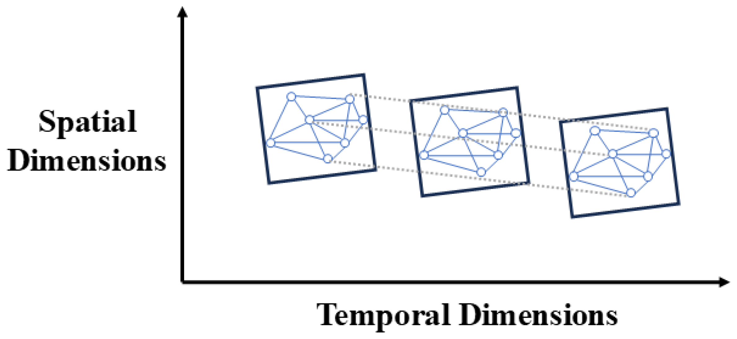
Each raster point in G generates a sequence of pollutant concentrations with the same sampling frequency, which forms a graphical sequence of data in Figure 9.

3.3.2. The Improved GCN

Standard GCNs often face challenges such as over-smoothing in deep architectures and limited receptive fields in shallow ones. To address these theoretical limitations, we introduce two key modifications to our GCN filter, inspired by recent advances in graph neural networks [44,45]. From a dynamical systems perspective, our iterative GCN layers learn to map inputs to stable attractors, which theoretically supports the model’s robustness in multi-step forecasting as follows [46]:
(1)
To mitigate over-smoothing, where node features become indistinguishable after many layers, we adjust the weight of self-loops by introducing a parameter p [ 0 , 1 ] [47]. By re-distributing weights between a node and its neighbors, we can explicitly control the amount of information retained from the node itself in each layer. The modified adjacency matrix W is defined as
W i j = p · exp d i j 2 σ 2 , i j and exp d i j 2 σ 2 ε 1 p , i = j .
When p approaches 1, the contribution of a node’s neighbors is emphasized, whereas a p value closer to 0 increases the weight of its self-information. After extensive testing, we found that the optimal value of p is approximately 0.91 , which effectively balances these influences for our task.
(2)
To expand the receptive field of the graph convolution without excessively deepening the model, we incorporate multi-hop neighborhood connections. By applying the normalized adjacency matrix K times, the model can directly capture information from up to K-hop neighbors in a single layer. This approach theoretically enhances the model’s ability to capture larger-scale spatial dependencies, which are crucial for regional pollution modeling [44].
While the adjacency matrix W ˜ (which is W in our case) defines the connections, using it directly can lead to numerical instabilities. To address this, we use the symmetrically normalized adjacency matrix, A ^ = D ˜ 1 / 2 W ˜ D ˜ 1 / 2 , a formulation derived from graph Laplacian theory. This normalization effectively averages neighbor features, ensuring a stable propagation process.
This multi-hop operation is applied using the modified adjacency matrix W (defined in Equation (8)), which already includes self-loop adjustments. For clarity, let W ˜ = W and D ˜ be its corresponding degree matrix. The operation is defined as
H ( L ) = σ D ˜ 1 / 2 W ˜ D ˜ 1 / 2 K H ( L 1 ) Θ ( L ) .
As shown in Equation (9), the normalized adjacency matrix is applied K times to expand the receptive field of the convolutional kernel up to K-hops. We tested seven different values for K, namely K = 1, 2, 3, 4, 5, 6, and 7. By observing the prediction results on the validation dataset, we found that the minimum error was achieved when K = 5. This specific value of K enables the model to capture relevant information from 5-hop neighborhoods efficiently.

3.3.3. GC-GRU

To overcome the gradient vanishing and explosion problems inherent in standard RNNs, gated mechanisms like those in LSTM and GRU are essential. In this work, we selected GRU to capture temporal dynamics. Theoretically, GRU possesses a simpler architecture with fewer gates (an update gate and a reset gate) compared to LSTM. This reduced complexity leads to fewer model parameters, which not only accelerates the training process but also mitigates the risk of overfitting, a crucial consideration for our complex, multi-source dataset [48,49].
The GC-GRU module in this work consists of the following components:
  • The core of our temporal modeling component is the GC-GRU cell. This module enhances the conventional GRU structure by making its gating mechanisms spatially aware. Instead of standard matrix multiplications, graph convolution operations ( 🟉 G ) are integrated into the update and reset gates. This modification allows each GRU to aggregate information not only from its own past state but also from its spatial neighbors at the current time step, thereby learning a unified spatio-temporal representation.
    The update gate u ˜ ( t ) and reset gate r ˜ ( t ) are computed as follows [48]:
    u ˜ ( t ) = σ Θ u 🟉 G X ( t ) , H ( t 1 ) + b u .
    r ˜ ( t ) = σ Θ r 🟉 G X ( t ) , H ( t 1 ) + b r .
    The candidate hidden state C ˜ ( t ) is then calculated using the reset gate to modulate the influence of the previous hidden state:
    C ˜ ( t ) = tanh Θ c 🟉 G X ( t ) , r ˜ ( t ) H ( t 1 ) + b c .
    Finally, the new hidden state H ( t ) is produced by the update gate, which balances information from the previous state and the current candidate state:
    H ( t ) = u ˜ ( t ) H ( t 1 ) + 1 u ˜ ( t ) C ˜ ( t ) ,
    where X ( t ) is the input feature matrix at time t, and H ( t 1 ) is the hidden state from the previous time step. The symbol 🟉 G denotes the graph convolution operation [50], σ is the Sigmoid activation function, and ⊙ represents the element-wise (Hadamard) product. The terms Θ u , Θ r , Θ c are the learnable weight matrices for their respective gates.
    The integration of graph convolution in this framework allows the GRU to effectively model spatio-temporal dependencies in graph-structured data, addressing challenges for traditional sequence-based architectures [48]. Figure 10 shows the GRU network cell structure.
  • Series connection of loop units: all GC-GRU cells are connected in series in chronological order, and the output of each unit is used as the input of the next unit to ensure the temporal continuity. With this structural design, the model is able to process inputs from different time steps and gradually establish global temporal dependencies. Figure 11 illustrates the architecture of the GC-GRU network.
  • Multi-Layer Architecture: To enhance the model’s capacity for learning complex patterns, multiple GC-GRU layers can be stacked. A ReLU activation function is applied between each layer to improve the model’s nonlinear representation capabilities. Finally, the output from the last GC-GRU layer is processed by a fully connected layer to generate the final predictions.

3.3.4. Seq2Seq

RNN has attracted a lot of attention in sequence data modeling because of its ability to effectively relate contextual information in sequence data [51]. The Seq2Seq model is one of the important extensions of RNN. The model compresses the input information into a fixed-length context vector through an encoder and then decodes it into the target sequence through a decoder. Usually, the Seq2Seq model uses two RNN models as an encoder and a decoder, respectively, and the last hidden state of the encoder is used as the overall context information [48].
In this study, both the encoder and decoder are implemented using GRU networks. GRU controls the information flow by setting update gates and reset gates to effectively mitigate the gradient vanishing or gradient explosion problems that may be encountered in long sequence processing. GRU performs well in dealing with long-time dependencies and has high training efficiency.
Within this framework, a GCN serves as the initial module to extract spatial relationships from the input data. The extracted spatial features are then organized into a time series matrix, which serves as the input for the encoder. The encoder, implemented using GC-GRUs, processes the input sequence ( X ( 1 ) , X ( 2 ) , , X ( T ) ) one time step at a time. During each iteration at time step t, the encoder generates an output vector, O t , which is the hidden state from its final layer. Crucially, unlike traditional Seq2Seq models that only use the final hidden state, our encoder provides the entire sequence of these output vectors, O = ( O 1 , O 2 , , O T ) , to the subsequent attention mechanism. This sequence provides a rich, contextual representation of the full input history, which is essential for the decoder to selectively focus on relevant information. This iterative approach continues until the entire sequence is fully analyzed, providing a comprehensive representation of the input data.
The decoder is initialized using the encoder’s final hidden state as its initial state: the output of each step becomes the input for the next step. It introduces potential error accumulation due to reliance on model-generated values. To address this, the decoder integrates the spatio-temporal context matrix produced by the encoder, ensuring that each prediction step considers both historical temporal patterns and spatial correlations extracted by the GCN module. A schematic representation of the seq2Seq model is shown in Figure 12.

3.3.5. Attention Mechanism

The seq2seq framework faces a limitation where the context vectors cannot fully capture the entire information present in the input sequence, thereby restricting the decoder’s performance during the decoding process. Attention mechanisms were found to be effective in mitigating information decay in sequence prediction models [52]. Because the encoder distributes critical information across its output vectors at each time step, the attention mechanism enables the decoder to move beyond sole dependence on context vectors. Instead, it integrates all encoder output vectors across time steps, applying weighted coefficients to calculate weighted sums. This process ensures that the decoder focuses on the most relevant information for the current time step. The attention mechanism focuses on the correlation between the value x k in the target sequence at a certain time and the dependency sequence x t s t e = [ x t s , , x t e ] , with the correlation represented by a set of attention weights a t s t e = [ a t s , , a t e ] [52]. Each element in the dependency sequence x t s t e has the same dimensionality d x as the target value x k . The target value x k and the elements in the dependency sequence x t s t e are projected into parameter spaces:
Q = x k W Q ,
K = x t s t e W K ,
V = x t s t e W V ,
where W Q is the parameter matrix of the query with dimensions d x × d q , W K is the parameter matrix of the key with dimensions d x   ×   d k , and W V is the parameter matrix of the value with dimensions d x   ×   d v , and d q   =   d k   =   d v .
The roles of W Q , W K and W V are weight matrices in fully connected neural networks and need to be updated through backpropagation. The target value, when multiplied with the query parameter matrix, projects the target value x k from dimension d x into a vector Q of dimension d q . Similarly, the matrix x t s t e is projected into a matrix K with element dimensions d k and into a matrix V with element dimensions d v . Both K and V represent different representations of the dependency sequence x t s t e . The difference is that K is used to quantify the relationship between the target value and the dependency sequence, serving as the basis for computing the attention weights, while the variable V is used to employ to compute the weighted sum of values derived from the dependency sequence, forming the output of the attention mechanism.
The relationship between the target value and the dependency sequence is defined as
a t s t e t k = softmax Q K d k ,
where softmax is the activation function used in deep learning, which normalizes the data to the range (0,1).
softmax ( x ) = e x j e j ,
where a t s t e t k represents the attention weight of the target value d x for each time step in the dependency sequence x t s t e . The stronger the correlation, the higher the attention weight. The attention vector is derived by computing the weighted sum of the attention weight matrix and the elements of the dependency sequence.
Attention = a t s t e t k V .
In order to improve the expression ability of attention between target values and dependent sequences and to enhance the breadth and depth of attention, the concept of multi-head attention. This approach involves utilizing H parameter matrices ( W Q , W K , W V ) to compute H independent attention mechanisms based on the same set of target values and dependency sequences, resulting in H attention vectors. Subsequently, the H attention vectors are concatenated to form a unified vector, representing the final output of the attention mechanism.

3.4. STGCA Model

The GCA model is proposed in this study, and it is structured with three main modules: GCN, a GRU-based encoder and a GRU-based decoder.
The GRU decoder integrates a multi-attention mechanism designed to model complex connections between input and output sequences over multiple steps, enhancing the precision of the decoding process. A multi-head self-attention mechanism is specifically embedded in the GRU decoder to form dependencies between the current time step’s input and all prior decoded outputs.
This multi-attention mechanism enables the model to capture both intra-sequence and cross-sequence dependencies, enhancing its ability to decode complex temporal relationships effectively.
Figure 13 illustrates the architecture of the GCA model. During prediction mode, the model operates autoregressively, meaning the output from the previous time step serves as the input for the next. The decoding process proceeds as follows:
  • Initialization: The hidden state of the decoder is initialized with the final hidden state vector from the encoder’s last time step. A special start-of-sequence token is used as the initial input to begin the generation process.
  • Decoder Self-Attention: At each decoding step t, the decoder first employs a self-attention mechanism. It uses its current state to attend to the sequence of all previously generated outputs ( y 0 , , y t 1 ). This step allows the decoder to consider the context of its own predictions so far.
  • Encoder–Decoder Attention: Subsequently, the decoder uses an attention mechanism to consult the source information. The decoder’s current hidden state is used as the “query” to attend to the entire sequence of the encoder’s output vectors. This produces a context vector that captures the most relevant input information needed for the current prediction.
  • Prediction and Iteration: The context vector obtained from the previous step is combined with the decoder’s current hidden state. This combined vector is then passed through a final fully connected layer to generate the prediction for the current time step, y t . This new output, y t , will then be used as the input for the next decoding step.

3.5. Experimental Configurations

All experiments are conducted on a Windows 11 workstation equipped with an Intel i7-13700 CPU (5.0 GHz), an NVIDIA GeForce RTX 4060 GPU with 8 GB, and 32 GB RAM. Data processing, model construction, and training are implemented using Python 3.9 with open-source libraries including Pandas 2.2.3, Numpy 2.2.6, and PyTorch 2.7.0.
The dataset is sequentially split into training, validation, and testing sets with ratios of 60%, 20%, and 20%, respectively, without shuffling to preserve temporal continuity. The selection of key hyperparameters was based on an empirical grid search. For instance, while several candidates for the observation window were tested, the 30-day window was ultimately selected, as it provided an optimal balance between capturing sufficient historical context and maintaining computational efficiency. For the loss function, MAE was selected [53], which is a commonly used and effective metric in the field of air pollution forecasting. Early stopping is employed to prevent overfitting, terminating training if validation loss does not improve by at least 1 × 10⁻⁴ over 50 consecutive epochs. The final hyperparameter values are summarized in Table 4. This configuration ensures accurate and stable multi-step PM2.5 concentration prediction, fully leveraging the STGCA architecture’s strength in modeling complex spatio-temporal dependencies.

4. Experimental Design and Validation

4.1. Experimental Design

Ablation Experiments

To evaluate the contribution of each component of the STGCA model for multi-step prediction of PM2.5 concentration, we conduct ablation experiments focusing on recurrent units, convolution methods, graph convolution filters, and the attention mechanism. The default backbone of our proposed STGCA model, which serves as the benchmark in these experiments, is composed of a GC-GRU recurrent unit, the Improved Convolution (IConv) method, a Dual Random Walk Filter (DRWF), and the integrated spatio-temporal attention mechanism. Each of the following experiments modifies one of these components to assess its impact.
  • Comparison between GC-LSTM and GC-GRU
    To explore the differences between LSTM and GRU in prediction accuracy, we compare the GC-LSTM with GC-GRU models. Table 5 presents the performance comparison between the GC-LSTM and GC-GRU models for PM2.5 prediction tasks. The results demonstrate that the GC-GRU model outperforms the GC-LSTM model across all metrics. Specifically, GC-GRU achieves lower RMSE, MAPE, TIC and higher IA values indicating better accuracy in predicting PM2.5 concentrations. This indicates that the GC-GRU has shown superior accuracy over GC-LSTM in prediction tasks.
  • Convolution methods
    In the graph convolution module, we test Chebyshev polynomial convolution (CConv) [54], diffusion convolution (DConv) [55], and our proposed IConv, which is detailed in Section 3.3.2. Our improved convolution method achieved the best performance across all metrics (Table 6).
  • Graph Convolution filter
    We further investigated three types of graph convolution filters to understand their effect on capturing spatial dependencies: the standard Laplacian Filter (LF), the Random Walk Filter (RWF), and DRWF. The RWF and DRWF are based on the diffusion process defined in [56]. The DRWF extends the standard random walk by considering both forward and backward diffusion directions, allowing more comprehensive modeling of spatial dependencies across the graph [56]. The DRWF demonstrated superior performance, highlighting its better ability to capture spatial dependencies (Table 7).
  • Attention mechanism
    Finally, we assess the effect of the attention mechanism by comparing the STGCA model with STGC, without the attention mechanism. The attention-enhanced STGCA model demonstrated improved accuracy by dynamically weighting important historical data, as shown in Table 8.
    The ablation experiments demonstrate that all the introduced IConv, DRWF and attention mechanisms significantly contribute to enhancing the proposed STGCA model’s predictive accuracy for PM2.5 concentrations. By jointly improving the model’s capacity to capture complex spatial and temporal dependencies, our proposed strategies achieve high performance in spatio-temporal prediction tasks.

4.2. Comparative Experiments

To further evaluate the effectiveness of the proposed STGCA model, we conducted comparative experiments with several advanced spatio-temporal prediction models, including VAR [57], FCLSTM [58], ASTGCN [59], MTGNN [60], and MTGODE [61] from other scholars. These models are widely used in the field of spatio-temporal forecasting and provide a solid baseline for comparison.
Each model was trained on the same dataset with identical preprocessing procedures. For shared hyperparameters, we applied the same grid search strategy to identify the optimal values. Other model-specific hyperparameters were set to their default values to ensure consistency and fairness in comparison.

Performance Comparisons Among Prediction Models

Table 9 presents the multi-step prediction performance of the six different models. This table provides insight into how each model performs over extended forecasting horizons, allowing us to evaluate their effectiveness in handling sequential dependencies across multiple steps.
The comparative experiments validate that the STGCA model provides a substantial improvement over other advanced models in PM2.5 concentrations prediction. It consistently achieves better evaluation indicators compared with benchmark models, indicating superior prediction accuracy in both single-step and multi-step forecasting. Benefiting from its attention mechanism and improved convolutional layers, STGCA is better equipped to capture complex temporal dependencies, as evidenced by its overall stronger performance across multiple evaluation metrics in the multi-step setting. Moreover, while other models exhibit significant performance degradation in multi-step forecasting, STGCA maintains relatively stable results, demonstrating its robustness and enhanced ability to model long-term dependencies. While the simpler VAR model is the fastest, its prediction accuracy is considerably lower. Among the deep learning models, our proposed STGCA (1602s) demonstrates a competitive advantage, being notably faster than more complex baselines like ASTGCN (1855s), MTGNN (2160s), and MTGODE (2450s) while delivering state-of-the-art accuracy. These combined strengths in both accuracy and efficiency make STGCA highly suitable for complex environmental forecasting tasks.

4.3. Comparisons Between Prediction and Observation

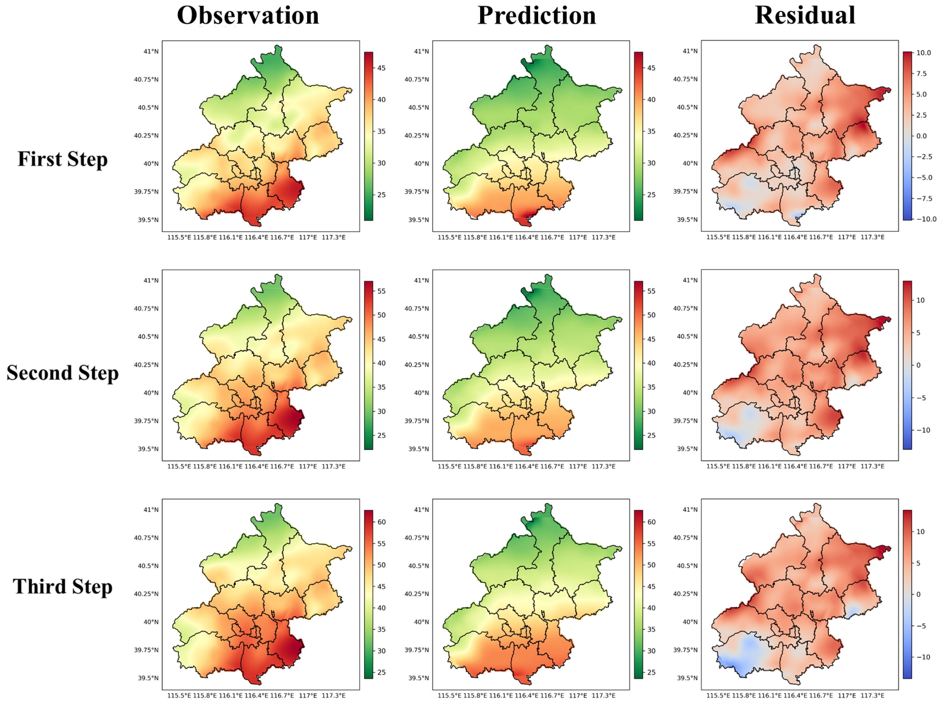
To visually assess the model’s performance, a representative case study for a multi-step forecast is presented in Figure 14. The figure compares the spatial distributions of observed PM2.5 concentrations, the model’s predictions, and the resulting residuals (observation–prediction) over a three-day horizon. In this example, the model effectively captures the overall spatial patterns and temporal dynamics, with predictions closely aligning with the actual measurements.
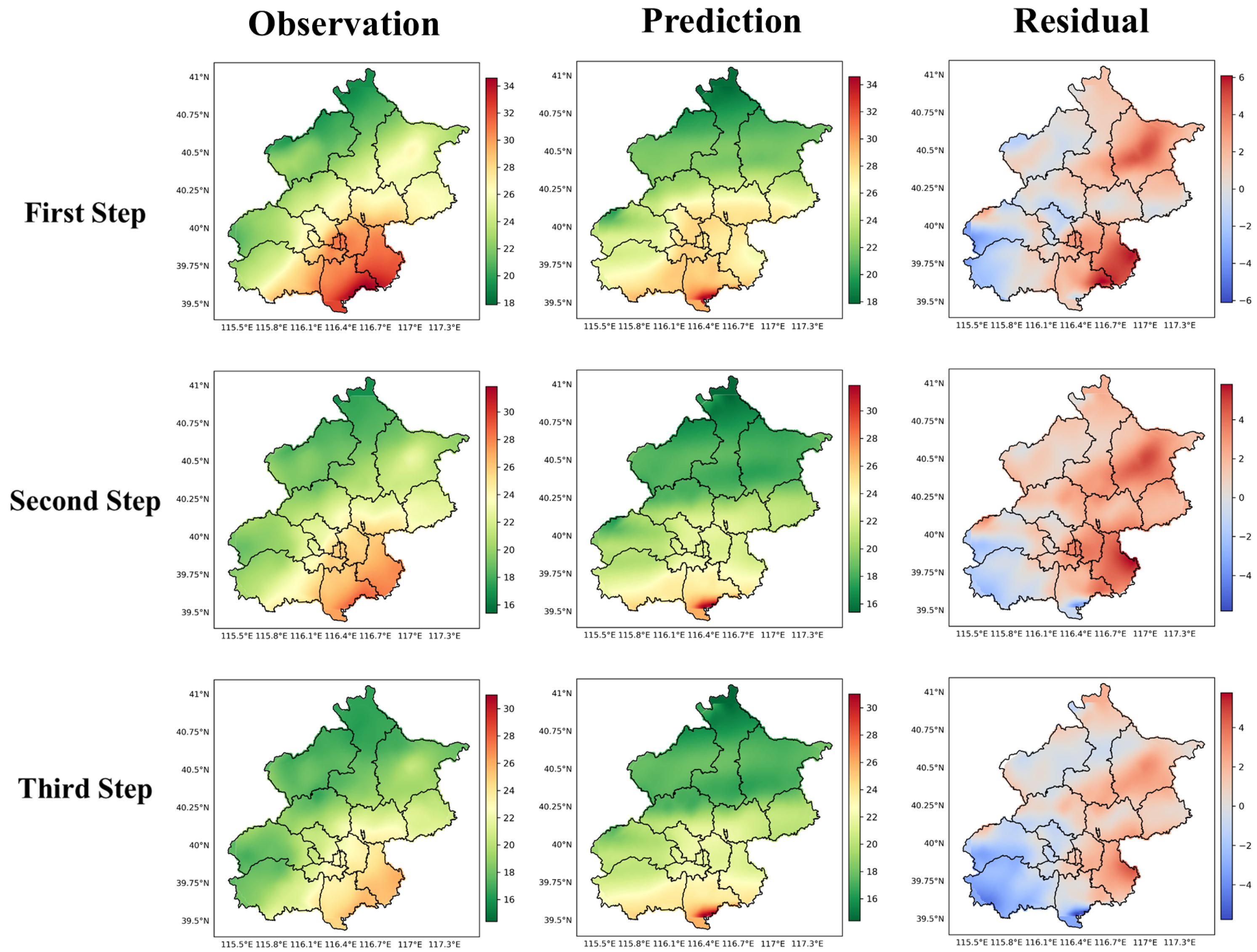
Furthermore, to provide a more comprehensive evaluation, additional randomly selected prediction examples are included in Appendix A (Figure A1 and Figure A2). The residual maps in these cases reveal similar error patterns. Overall, the prediction errors are small across most regions, and the model’s performance remains robust as the forecast step increases. In general, no obvious systematic biases have been shown across region and concentration range.
Based on the experimental results, the STGCA model has effectively learned the spatio-temporal dependencies of PM2.5 pollution and demonstrated excellent robustness in regional, multi-step forecasting. Although STGCA successfully captures the overall pollution patterns and achieves low prediction errors, it has limitations in distinguishing the precise boundaries of sharp concentration gradients and in capturing extreme values. These results confirm the model’s potential as a reliable tool for regional air quality forecasting.

5. Conclusions

In this work, we proposed the STGCA model, which integrates a spatio-temporal attention module, an improved graph convolution, and a GRU-based seq2seq framework. Compared with existing models, STGCA demonstrates superior capability in modeling complex spatio-temporal dependencies. The experimental results validate its effectiveness, achieving significantly lower prediction errors across multi-step PM2.5 forecasting tasks. For the first (second, third) step, our model achieved RMSE of 4.21 (5.08, 6.54), MAE of 3.11 (3.69, 4.61), MAPE of 11.41% (13.34%, 16.62%), IA of 0.98 (0.97, 0.95) and TIC of 0.06 (0.08, 0.10), respectively, outperforming the baseline models.
Unlike traditional approaches that focus on sparse station-based point-wise predictions, STGCA advances the state-of-the-art by enabling high-resolution regional “surface-level” forecasting through learning from spatially rasterized grids. This shift from point to grid prediction not only improves the spatial granularity but also significantly enhances prediction accuracy. The model effectively captures complex spatio-temporal dependencies, enabling comprehensive coverage over urban areas and offering stronger support for air quality management in large-scale heterogeneous environments; while multi-source data, including remote sensing and meteorological information, are incorporated, the key innovation lies in transitioning to fine-grained surface prediction, breaking through the limitations of traditional sparse monitoring data.
Although the proposed framework demonstrates promising results, some improvements will be considered in future research. Firstly, the validation of this study was conducted in Beijing; while Beijing serves as a representative and complex case study, future work will focus on evaluating the model’s robustness and generalizability across more diverse urban environments with different data characteristics. Secondly, to further refine the experimental process, we plan to introduce automated hyperparameter optimization techniques. Thirdly, a thorough analysis of feature importance, for instance through a feature-level ablation study, will be conducted to provide deeper insights into the key drivers of PM2.5 pollution. Finally, we will explore methods for uncertainty quantification, such as generating prediction intervals, to make the model more practical and powerful for decision-making under uncertainty.

Author Contributions

Funding acquisition, X.M. and H.L.; methodology, X.G., X.M., and H.L.; software, X.G.; writing—original draft, X.G., X.M., and H.L.; writing—review and editing, X.G., X.M., and H.L. All authors have read and agreed to the published version of the manuscript.

Funding

This work is supported by the Hainan Provincial Natural Science Foundation of China (grant numbers 623RC455, 623RC457, 425QN244), the Scientific Research Fund of Hainan University (grant numbers KYQD (ZR)-22096, KYQD(ZR)-22097), and the Lanzhou University-Hainan University Technical Service Project (HD-KYH-2024424).

Institutional Review Board Statement

Not applicable.

Informed Consent Statement

Not applicable.

Data Availability Statement

The datasets presented in this study can be found in the following online repositories. Further inquiries can be directed to the corresponding author. The China High Air Pollutants (CHAP) dataset and the Aerosol Optical Depth (AOD)-LGHAP dataset are both publicly available from the National Earth System Science Data Centre, which can be accessed at https://www.aers-cloud.org.cn/ (accessed on 15 August 2024). The ERA5-Land meteorological data are publicly available from the Copernicus Climate Data Store at https://cds.climate.copernicus.eu/ (accessed on 15 August 2024). The Normalized Difference Vegetation Index (NDVI) data are publicly available from NASA’s Earth Observing System (NEO) platform at https://neo.gsfc.nasa.gov/ (accessed on 15 August 2024). The source code developed to reproduce the results of this study has been made publicly available on GitHub and can be accessed at the following repository: https://github.com/chuxina7-aiguo/STGCA.git (accessed on 15 August 2024).

Conflicts of Interest

The authors declare no conflicts of interest.

Appendix A

Figure A1. Comparison of observation, prediction and residual for case 1.
Make 07 00088 g0a1
Figure A2. Comparison of observation, prediction and residual for case 2.
Make 07 00088 g0a2

References

  1. Hill, W.; Lim, E.L.; Weeden, C.E.; Lee, C.; Augustine, M.; Chen, K.; Kuan, F.C.; Marongiu, F.; Evans, E.J., Jr.; Moore, D.A.; et al. Lung adenocarcinoma promotion by air pollutants. Nature 2023, 616, 159–167. [Google Scholar] [CrossRef] [PubMed]
  2. Mo, X.; Li, H.; Zhang, L.; Qu, Z. Environmental impact estimation of PM2.5 in representative regions of China from 2015 to 2019: Policy validity, disaster threat, health risk, and economic loss. Air Qual. Atmos. Health 2021, 14, 1571–1585. [Google Scholar] [CrossRef]
  3. Fann, N.L.; Nolte, C.G.; Sarofim, M.C.; Martinich, J.; Nassikas, N.J. Associations between simulated future changes in climate, air quality, and human health. JAMA Netw. Open 2021, 4, e2032064. [Google Scholar] [CrossRef] [PubMed]
  4. Yarragunta, Y.; Francis, D.; Fonseca, R.; Nelli, N. Evaluation of the WRF-Chem performance for the air pollutants over the United Arab Emirates. Atmos. Chem. Phys. 2025, 25, 1685–1709. [Google Scholar] [CrossRef]
  5. Bhatti, U.A.; Yan, Y.; Zhou, M.; Ali, S.; Hussain, A.; Qingsong, H.; Yu, Z.; Yuan, L. Time series analysis and forecasting of air pollution particulate matter (PM2.5): An SARIMA and factor analysis approach. IEEE Access 2021, 9, 41019–41031. [Google Scholar] [CrossRef]
  6. Abdullah, S.; Napi, N.N.L.M.; Ahmed, A.N.; Mansor, W.N.W.; Mansor, A.A.; Ismail, M.; Abdullah, A.M.; Ramly, Z.T.A. Development of multiple linear regression for particulate matter (PM10) forecasting during episodic transboundary haze event in Malaysia. Atmosphere 2020, 11, 289. [Google Scholar] [CrossRef]
  7. Xu, X.; Tong, T.; Zhang, W.; Meng, L. Fine-grained prediction of PM2.5 concentration based on multisource data and deep learning. Atmos. Pollut. Res. 2020, 11, 1728–1737. [Google Scholar] [CrossRef]
  8. Masood, A.; Ahmad, K. A model for particulate matter (PM2.5) prediction for Delhi based on machine learning approaches. Procedia Comput. Sci. 2020, 167, 2101–2110. [Google Scholar] [CrossRef]
  9. Liu, Z.; Huang, X.; Wang, X. PM2.5 prediction based on modified whale optimization algorithm and support vector regression. Sci. Rep. 2024, 14, 23296. [Google Scholar] [CrossRef] [PubMed]
  10. Gao, Z.; Do, K.; Li, Z.; Jiang, X.; Maji, K.J.; Ivey, C.E.; Russell, A.G. Predicting PM2.5 levels and exceedance days using machine learning methods. Atmos. Environ. 2024, 323, 120396. [Google Scholar] [CrossRef]
  11. Pan, B. Application of XGBoost algorithm in hourly PM2.5 concentration prediction. IOP Conf. Ser. Earth Environ. Sci. 2018, 113, 012127. [Google Scholar] [CrossRef]
  12. Maleki, H.; Sorooshian, A.; Goudarzi, G.; Baboli, Z.; Tahmasebi Birgani, Y.; Rahmati, M. Air pollution prediction by using an artificial neural network model. Clean Technol. Environ. Policy 2019, 21, 1341–1352. [Google Scholar] [CrossRef] [PubMed]
  13. Li, H.; Wang, J.; Li, R.; Lu, H. Novel analysis–forecast system based on multi-objective optimization for air quality index. J. Clean. Prod. 2019, 208, 1365–1383. [Google Scholar] [CrossRef]
  14. Kow, P.Y.; Chang, L.C.; Lin, C.Y.; Chou, C.C.K.; Chang, F.J. Deep neural networks for spatiotemporal PM2.5 forecasts based on atmospheric chemical transport model output and monitoring data. Environ. Pollut. 2022, 306, 119348. [Google Scholar] [CrossRef] [PubMed]
  15. Zhang, K.; Cao, H.; Thé, J.; Yu, H. A hybrid model for multi-step coal price forecasting using decomposition technique and deep learning algorithms. Appl. Energy 2022, 306, 118011. [Google Scholar] [CrossRef]
  16. Zhang, K.; Thé, J.; Xie, G.; Yu, H. Multi-step ahead forecasting of regional air quality using spatial-temporal deep neural networks: A case study of Huaihai Economic Zone. J. Clean. Prod. 2020, 277, 123231. [Google Scholar] [CrossRef]
  17. Lim, B.; Zohren, S. Time-series forecasting with deep learning: A survey. Philos. Trans. R. Soc. A 2021, 379, 20200209. [Google Scholar] [CrossRef]
  18. Abirami, S.; Chitra, P. Regional air quality forecasting using spatiotemporal deep learning. J. Clean. Prod. 2021, 283, 125341. [Google Scholar] [CrossRef]
  19. Acikgoz, H. A novel approach based on integration of convolutional neural networks and deep feature selection for short-term solar radiation forecasting. Appl. Energy 2022, 305, 117912. [Google Scholar] [CrossRef]
  20. Sayeed, A.; Choi, Y.; Eslami, E.; Lops, Y.; Roy, A.; Jung, J. Using a deep convolutional neural network to predict 2017 ozone concentrations, 24 hours in advance. Neural Netw. 2020, 121, 396–408. [Google Scholar] [CrossRef] [PubMed]
  21. Mo, X.; Li, H.; Zhang, L. Design a regional and multistep air quality forecast model based on deep learning and domain knowledge. Front. Earth Sci. 2022, 10, 995843. [Google Scholar] [CrossRef]
  22. Ehteram, M.; Ahmed, A.N.; Khozani, Z.S.; El-Shafie, A. Graph convolutional network–Long short term memory neural network-multi layer perceptron-Gaussian progress regression model: A new deep learning model for predicting ozone concertation. Atmos. Pollut. Res. 2023, 14, 101766. [Google Scholar] [CrossRef]
  23. Chen, Q.; Ding, R.; Mo, X.; Li, H.; Xie, L.; Yang, J. An adaptive adjacency matrix-based graph convolutional recurrent network for air quality prediction. Sci. Rep. 2024, 14, 4408. [Google Scholar] [CrossRef] [PubMed]
  24. Bai, H.; Shi, Y.; Seong, M.; Gao, W.; Li, Y. Influence of spatial resolution on satellite-based PM2.5 estimation: Implications for health assessment. Remote Sens. 2022, 14, 2933. [Google Scholar] [CrossRef]
  25. Wei, J.; Li, Z. China High Resolution High Quality PM2.5 Dataset (2000–2021); National Tibetan Plateau/Third Pole Environment Data Center: Beijing, China, 2023. [Google Scholar]
  26. Mathias, S.; Wayland, R. Fine Particulate Matter (PM2.5) Precursor Demonstration Guidance; Office of Air Quality Planning and Standards, United States Environmental Protection Agency: Washington, DC, USA, 2019. [Google Scholar]
  27. Muñoz Sabater, J.; Dutra, E.; Agustí-Panareda, A.; Albergel, C.; Arduini, G.; Balsamo, G.; Boussetta, S.; Choulga, M.; Harrigan, S.; Hersbach, H.; et al. ERA5-Land: A state-of-the-art global reanalysis dataset for land applications. Earth Syst. Sci. Data 2021, 13, 4349–4383. [Google Scholar] [CrossRef]
  28. Cai, W.; Li, K.; Liao, H.; Wang, H.; Wu, L. Weather conditions conducive to Beijing severe haze more frequent under climate change. Nat. Clim. Change 2017, 7, 257–262. [Google Scholar] [CrossRef]
  29. Bai, K.; Li, K.; Ma, M.; Li, K.; Li, Z.; Guo, J.; Chang, N.B.; Tan, Z.; Han, D. LGHAP: A Long-term Gap-free High-resolution Air Pollutants concentration dataset derived via tensor flow based multimodal data fusion. Earth Syst. Sci. Data Discuss. 2021, 2021, 1–39. [Google Scholar] [CrossRef]
  30. Zhang, X.; Friedl, M.A.; Schaaf, C.B.; Strahler, A.H.; Hodges, J.C.; Gao, F.; Reed, B.C.; Huete, A. Monitoring vegetation phenology using MODIS. Remote Sens. Environ. 2003, 84, 471–475. [Google Scholar] [CrossRef]
  31. Van Donkelaar, A.; Martin, R.V.; Brauer, M.; Kahn, R.; Levy, R.; Verduzco, C.; Villeneuve, P.J. Global estimates of ambient fine particulate matter concentrations from satellite-based aerosol optical depth: Development and application. Environ. Health Perspect. 2010, 118, 847–855. [Google Scholar] [CrossRef]
  32. Gong, C.; Xian, C.; Wu, T.; Liu, J.; Ouyang, Z. Role of urban vegetation in air phytoremediation: Differences between scientific research and environmental management perspectives. npj Urban Sustain. 2023, 3, 24. [Google Scholar] [CrossRef]
  33. Yao, R.; Wang, L.; Huang, X.; Sun, L.; Chen, R.; Wu, X.; Zhang, W.; Niu, Z. A robust method for filling the gaps in MODIS and VIIRS land surface temperature data. IEEE Trans. Geosci. Remote Sens. 2021, 59, 10738–10752. [Google Scholar] [CrossRef]
  34. Dickey, D.A.; Fuller, W.A. Distribution of the estimators for autoregressive time series with a unit root. J. Am. Stat. Assoc. 1979, 74, 427–431. [Google Scholar] [PubMed]
  35. Wang, W.; Zhao, S.; Jiao, L.; Taylor, M.; Zhang, B.; Xu, G.; Hou, H. Estimation of PM2.5 concentrations in China using a spatial back propagation neural network. Sci. Rep. 2019, 9, 13788. [Google Scholar] [CrossRef] [PubMed]
  36. Getis, A.; Aldstadt, J. Constructing the spatial weights matrix using a local statistic. Geogr. Anal. 2004, 36, 90–104. [Google Scholar] [CrossRef]
  37. Yang, H.; Zhu, Z.; Li, C.; Li, R. A novel combined forecasting system for air pollutants concentration based on fuzzy theory and optimization of aggregation weight. Appl. Soft Comput. 2020, 87, 105972. [Google Scholar] [CrossRef]
  38. Zhang, K.; Yang, X.; Cao, H.; Thé, J.; Tan, Z.; Yu, H. Multi-step forecast of PM2.5 and PM10 concentrations using convolutional neural network integrated with spatial–temporal attention and residual learning. Environ. Int. 2023, 171, 107691. [Google Scholar] [CrossRef]
  39. Bahdanau, D. Neural machine translation by jointly learning to align and translate. arXiv 2014, arXiv:1409.0473. [Google Scholar]
  40. Woo, S.; Park, J.; Lee, J.Y.; Kweon, I.S. Cbam: Convolutional block attention module. In Proceedings of the European Conference on Computer Vision (ECCV), Munich, Germany, 8–14 September 2018; pp. 3–19. [Google Scholar]
  41. Wang, H.; Chen, Z.; Zhang, P. Spatial Autocorrelation and Temporal Convergence of PM2.5 Concentrations in Chinese Cities. Int. J. Environ. Res. Public Health 2022, 19, 13942. [Google Scholar] [CrossRef]
  42. Chae, S.; Shin, J.; Kwon, S.; Lee, S.; Kang, S.; Lee, D. PM10 and PM2.5 real-time prediction models using an interpolated convolutional neural network. Sci. Rep. 2021, 11, 11952. [Google Scholar] [CrossRef] [PubMed]
  43. Zhou, J.; Cui, G.; Hu, S.; Zhang, Z.; Yang, C.; Liu, Z.; Wang, L.; Li, C.; Sun, M. Graph neural networks: A review of methods and applications. AI Open 2020, 1, 57–81. [Google Scholar] [CrossRef]
  44. Wu, F.; Souza, A.; Zhang, T.; Fifty, C.; Yu, T.; Weinberger, K. Simplifying graph convolutional networks. In Proceedings of the International Conference on Machine Learning, PMLR, Long Beach, CA, USA, 9–15 June 2019; pp. 6861–6871. [Google Scholar]
  45. Chen, Z.M.; Wei, X.S.; Wang, P.; Guo, Y. Multi-label image recognition with graph convolutional networks. In Proceedings of the IEEE/CVF Conference on Computer Vision and Pattern Recognition, Long Beach, CA, USA, 15–20 June 2019; pp. 5177–5186. [Google Scholar]
  46. Marino, R.; Buffoni, L.; Chicchi, L.; Giambagli, L.; Fanelli, D. Stable attractors for neural networks classification via ordinary differential equations (SA-nODE). Mach. Learn. Sci. Technol. 2024, 5, 035087. [Google Scholar] [CrossRef]
  47. Gasteiger, J.; Bojchevski, A.; Günnemann, S. Predict then propagate: Graph neural networks meet personalized pagerank. arXiv 2018, arXiv:1810.05997. [Google Scholar]
  48. Cho, K. Learning phrase representations using RNN encoder-decoder for statistical machine translation. arXiv 2014, arXiv:1406.1078. [Google Scholar] [CrossRef]
  49. Chung, J.; Gulcehre, C.; Cho, K.; Bengio, Y. Empirical evaluation of gated recurrent neural networks on sequence modeling. arXiv 2014, arXiv:1412.3555. [Google Scholar] [CrossRef]
  50. Kipf, T.N.; Welling, M. Semi-supervised classification with graph convolutional networks. arXiv 2016, arXiv:1609.02907. [Google Scholar]
  51. Sutskever, I. Sequence to Sequence Learning with Neural Networks. arXiv 2014, arXiv:1409.3215. [Google Scholar] [CrossRef]
  52. Vaswani, A.; Shazeer, N.; Parmar, N.; Uszkoreit, J.; Jones, L.; Gomez, A.N.; Kaiser, L.; Polosukhin, I. Attention is all you need. In Proceedings of the 31st International Conference on Neural Information Processing Systems, Long Beach, CA, USA, 4–9 December 2017; pp. 5998–6008. [Google Scholar]
  53. Goodfellow, I.; Bengio, Y.; Courville, A. Deep Learning; MIT Press: Cambridge, MA, USA, 2016. [Google Scholar]
  54. Defferrard, M.; Bresson, X.; Vandergheynst, P. Convolutional neural networks on graphs with fast localized spectral filtering. Adv. Neural Inf. Process. Syst. 2016, 29, 1386–1394. [Google Scholar]
  55. Atwood, J.; Towsley, D. Diffusion-convolutional neural networks. Adv. Neural Inf. Process. Syst. 2016, 29, 1993–2001. [Google Scholar]
  56. Li, Y.; Yu, R.; Shahabi, C.; Liu, Y. Diffusion convolutional recurrent neural network: Data-driven traffic forecasting. arXiv 2017, arXiv:1707.01926. [Google Scholar]
  57. Gholamzadeh, F.; Bourbour, S. Air pollution forecasting for Tehran city using Vector Auto Regression. In Proceedings of the 2020 6th Iranian Conference on Signal Processing and Intelligent Systems (ICSPIS), Mashhad, Iran, 23–24 December 2020; pp. 1–5. [Google Scholar]
  58. Yu, W.; Li, J.; Liu, Q.; Zhao, J.; Dong, Y.; Wang, C.; Lin, S.; Zhu, X.; Zhang, H. Spatial–Temporal Prediction of Vegetation Index With Deep Recurrent Neural Networks. IEEE Geosci. Remote Sens. Lett. 2022, 19, 1–5. [Google Scholar] [CrossRef]
  59. Guo, S.; Lin, Y.; Feng, N.; Song, C.; Wan, H. Attention based spatial-temporal graph convolutional networks for traffic flow forecasting. In Proceedings of the AAAI Conference on Artificial Intelligence, Honolulu, HI, USA, 27 January–1 February 2019; pp. 922–929. [Google Scholar]
  60. Wu, Z.; Pan, S.; Long, G.; Jiang, J.; Chang, X.; Zhang, C. Connecting the dots: Multivariate time series forecasting with graph neural networks. In Proceedings of the 26th ACM SIGKDD International Conference on Knowledge Discovery & Data Mining, Virtual Event, CA, USA, 23–27 August 2020; pp. 753–763. [Google Scholar]
  61. Jin, M.; Zheng, Y.; Li, Y.F.; Chen, S.; Yang, B.; Pan, S. Multivariate time series forecasting with dynamic graph neural odes. IEEE Trans. Knowl. Data Eng. 2022, 35, 9168–9180. [Google Scholar] [CrossRef]
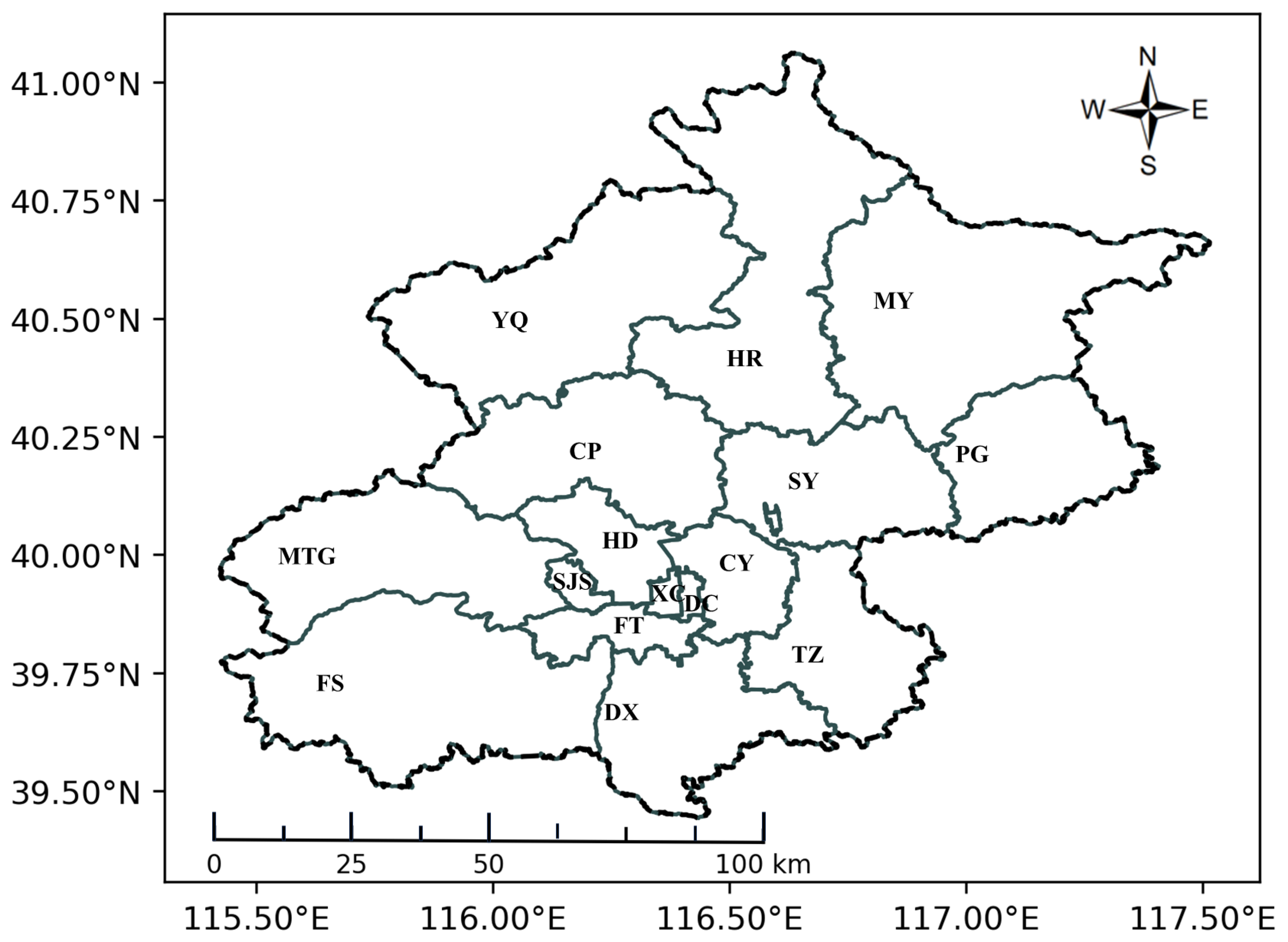
Figure 1. Geographical distribution of Beijing.
Make 07 00088 g001
Figure 2. PM2.5 concentration in Beijing.
Make 07 00088 g002
Figure 3. Global Moran’s index (I) scatter plot, showing a strong positive spatial autocorrelation ((I) = 0.85).
Make 07 00088 g003
Figure 4. LISA cluster map of PM2.5 concentrations.
Make 07 00088 g004
Figure 5. The framework of the STGCA.
Make 07 00088 g005
Figure 6. Spatial attention module.
Make 07 00088 g006
Figure 7. Temporal attention module.
Make 07 00088 g007
Figure 8. Spatio-temporal attention module.
Make 07 00088 g008
Figure 9. Spatio-temporal structure of air pollutant data.
Make 07 00088 g009
Figure 10. The structure of GRU.
Make 07 00088 g010
Figure 11. Graph convolutional gating layer.
Make 07 00088 g011
Figure 12. The architecture of Seq2Seq model.
Make 07 00088 g012
Figure 13. The architecture of GCA model.
Make 07 00088 g013
Figure 14. Comparisons among the observation, prediction and residual.
Make 07 00088 g014
Table 1. Experimental data and sources.
Data TypeVariableUnitSource
PollutantPM2.5µg/m3CHAP
ConcentrationPM10µg/m3CHAP
NO2µg/m3CHAP
COmg/m3CHAP
O3µg/m3CHAP
SO2µg/m3CHAP
MeteorologicalD2m°CECMWF ERA5
FactorT2m°CECMWF ERA5
TPmmECMWF ERA5
UWm/sECMWF ERA5
VWm/sECMWF ERA5
SPhPaECMWF ERA5
SSRMJ/m2ECMWF ERA5
OthersAOD CHAP
NDVI NEO
Table 2. ADF results of PM2.5 concentrations.
ADF Statistic1%5%10%p-Value
−5.9135−3.4314−2.8620−2.5670 2.61 × 10 7
Table 3. Definition and calculation formula of evaluation metrics.
MetricCalculation Formula
RMSE 1 N i = 1 N y i y i 2
MAE 1 N i = 1 N y i y i
MAPE 1 N i = 1 N y i y i y i
IA 1 i = 1 N y i y i 2 i = 1 N y i y ¯ + y i y ¯ 2
TIC 1 N i = 1 N y i y i 2 1 N i = 1 N y i 2 + 1 N i = 1 N y i 2
Note: N denotes the total number of forecasting samples. y i is the predicted data, and y i is the observed data. y ¯ represents the average of the observed data.
Table 4. Hhyperparameter selection.
Training ParametersMethod/Value
Observation window30 days
Prediction window3 days
Number of hidden layer neurons64
Activation function of convolutionalTanh
Activation function of fully connected layers in decoderReLU
Dropout ratio30%
Loss functionMAE
Optimization algorithmAdam
Initial learning rate0.001
Batch size128
Training epochs300
Table 5. Performance of GC-LSTM and GC-GRU.
Time StepModelRMSEMAEMAPEIATIC
First StepGC-LSTM5.633.9413.120.810.09
GC-GRU4.213.1111.410.980.06
Second StepGC-LSTM6.214.5114.200.780.11
GC-GRU5.083.6913.340.970.08
Third StepGC-LSTM7.025.1315.890.730.13
GC-GRU6.544.6116.620.950.10
Note: Bold values indicate the best performance for each metric.
Table 6. Performance of different convolutional approaches at different time steps.
Time StepModelRMSEMAEMAPEIATIC
First StepCConv7.335.4719.930.920.12
DConv7.735.2716.370.900.13
IConv4.213.1111.410.980.06
Second StepCConv8.896.1520.100.900.13
DConv8.106.3219.880.890.11
IConv5.083.6913.340.970.08
Third StepCConv9.407.6321.340.880.15
DConv9.657.7120.410.870.13
IConv6.544.6116.620.950.10
Note: Bold values indicate the best performance for each metric.
Table 7. Performance of graph convolution filters.
Time StepModelRMSEMAEMAPEIATIC
First StepLF5.574.3417.310.950.09
RWF6.905.3522.330.930.10
DRWF4.213.1111.410.980.06
Second StepLF6.805.5018.000.940.10
RWF7.205.6023.000.920.11
DRWF5.083.6913.340.970.08
Third StepLF7.005.7020.500.930.13
RWF7.505.8025.500.900.12
DRWF6.544.6116.620.950.10
Note: Bold values indicate the best performance for each metric.
Table 8. The impact of attention mechanism on prediction performance at different time steps.
Time StepModelRMSEMAEMAPEIATIC
First StepSTGC4.704.2213.890.930.09
STGCA4.213.1111.410.980.06
Second StepSTGC5.314.3814.260.920.10
STGCA5.083.6913.340.970.08
Third StepSTGC6.834.8917.020.910.11
STGCA6.544.6116.620.950.10
Note: Bold values indicate the best performance for each metric.
Table 9. Performance and efficiency comparison of six different models for PM2.5 multi-step prediction.
Time StepModelRMSEMAEMAPEIATICTime (s)
VAR8.134.9816.190.980.08221.5
FCLSTM8.105.9713.930.930.131480.7
First StepASTGCN7.464.729.000.840.171855.2
MTGNN7.545.4218.720.910.122160.4
MTGODE4.383.2210.680.980.072450.9
STGCA4.213.1111.410.980.061602.0
VAR11.517.0621.420.960.12221.5
FCLSTM9.506.6015.500.910.141480.7
Second StepASTGCN9.626.3612.000.880.161855.2
MTGNN7.772.3319.100.910.122160.4
MTGODE6.985.0316.430.940.102450.9
STGCA5.083.6913.340.970.081602.0
VAR14.559.1526.540.930.15221.5
FCLSTM10.007.2016.000.900.141480.7
Third StepASTGCN11.037.5821.000.700.281855.2
MTGNN9.476.9023.210.850.152160.4
MTGODE10.237.7928.560.820.152450.9
STGCA6.544.6116.620.950.101602.0
Note: Bold values indicate the best performance for each metric.
Disclaimer/Publisher’s Note: The statements, opinions and data contained in all publications are solely those of the individual author(s) and contributor(s) and not of MDPI and/or the editor(s). MDPI and/or the editor(s) disclaim responsibility for any injury to people or property resulting from any ideas, methods, instructions or products referred to in the content.