Abstract
The data landscape has changed, as more and more information is produced in the form of continuous data streams instead of stationary datasets. In this context, several online machine learning techniques have been proposed with the aim of automatically adapting to changes in data distributions, known as drifts. Though effective in certain scenarios, contemporary techniques do not generalize well to different types of data, while they also require manual parameter tuning, thus significantly hindering their applicability. Moreover, current methods do not thoroughly address drifts, as they mostly focus on concept drifts (distribution shifts on the target variable) and not on data drifts (changes in feature distributions). To confront these challenges, in this paper, we propose an AutoML Pipeline for Streams (AML4S), which automates the choice of preprocessing techniques, the choice of machine learning models, and the tuning of hyperparameters. Our pipeline further includes a drift detection mechanism that identifies different types of drifts, therefore continuously adapting the underlying models. We assess our pipeline on several real and synthetic data streams, including a data stream that we crafted to focus on data drifts. Our results indicate that AML4S produces robust pipelines and outperforms existing online learning or AutoML algorithms.
1. Introduction
Currently, more than ever before, technology plays an increasingly central role in daily life, making data a cornerstone of human activity. The amount of data to be exploited has increased tremendously, leading to a new era, that of big data. In addition to their large volume, big data are also characterized by high velocity and substantial variety [1], resulting from their production in continuous flows [2], known as data streams, while they may also arrive in various semi-structured or even unstructured formats.
The mining of these data streams is a challenging process because of their evolving characteristics. Apart from the large volume and possible variability, the distribution of the data may often undergo several changes, known as drifts. Drifts may represent changes that affect specific data variables (typically referred to as data drifts) or even, in a machine learning context, changes that affect the correlation between input and output variables (typically referred to as concept drifts) [3,4]. Either way, the research community has identified the need for machine learning techniques that are capable of adapting to these drifts [5].
Contemporary techniques for data streams, or so-called online machine learning algorithms, typically include mechanisms to identify drifts, which allow the algorithm to adapt to distribution shifts [6,7,8,9,10,11]. Though useful, these methods usually require manual configuration, while their performance is highly dependent on the dataset under analysis. On the other hand, AutoML approaches for data streams are few and rather limited [12,13,14,15,16,17]; most of them either do not adapt to drifts, or they focus only on concept drifts, while they may also employ a narrow selection of models (e.g., only trees) or introduce considerable latency when integrating distribution changes into the models.
In this work, we propose a methodology that confronts the aforementioned limitations. We design an AutoML Pipeline for Streams (AML4S), which involves different preprocessing techniques and online machine learning models, effectively making it able to handle a wide variety of data streams. All steps of our pipeline (i.e., preprocessing, model selection, hyperparameter tuning) are fully automated, while it also integrates a drift detection mechanism that can identify both data drifts and concept drifts, thus allowing our pipeline to adapt to any changes in the distribution of the data. Finally, to assess our methodology, we also craft a data stream generator to create synthetic datasets that include both data drifts and concept drifts. Our methodology is then compared with different online learning methods, as well as a contemporary AutoML approach.
The remainder of this paper is organized as follows. Section 2 provides background information and related work on data streams. Section 3 describes our proposed framework for an AutoML pipeline. Section 4 provides the results of our evaluation on different datasets. Section 5 discusses certain threats to validity and limitations, while Section 6 concludes this paper and provides ideas for future work.
2. Background and Related Work
As already mentioned, technological advancements have brought forth a new era in data mining and machine learning research; one where algorithms must be able to adapt to ever-evolving data streams. Click-through data, social media outputs, financial micro-transactions, and even IoT sensor data are only a few of the example applications that generate large amounts of data at high velocity [18]. In this context, a significant challenge faced by traditional (batch) machine learning models is that the distribution of the incoming data may shift at some point, e.g., a new product launch may significantly change the buying behavior of consumers, unexpected news may alter the stock price of a company, etc. These types of changes in distribution are commonly referred to as drifts [3,4]. Drifts can take various forms, as shown in Figure 1.
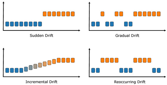
Figure 1.
Different types of drifts. Figure adapted from [4].
They can be sudden, where the distribution changes drastically in a small time frame, usually in response to an unexpected event, or the distribution can change gradually due to the inertia of the scenario, with the two distributions coexisting temporarily, (e.g., a new popular framework may replace another older one in user preference). Incremental drifts are also similar; however, they occur in cases where there is no clear transition between the two underlying data distributions, but rather the shift happens progressively and continuously (e.g., electricity/gas use throughout the autumn and winter months when the weather becomes progressively colder). Finally, a drift can even be reoccurring, meaning that previously observed distributions reappear occasionally, which is a common response to external changes that keep appearing at different points in time (e.g., a weather event may change the traffic conditions whenever it happens).
Another important distinction can be made based on the variables that are affected by the distribution change. In current literature, the two main categories of drifts recognized are concept drifts and data drifts [3,4], as shown in Figure 2 (current literature also provides other names for these drifts; e.g., data drifts are sometimes referred to as virtual drifts or feature drifts, while concept drifts are also known as label drifts [5]). In the context of a classification scenario, concept drifts signify changes in the correlation between the input variables (X) and the target output (y), i.e., a shift in the conditional distribution . As a result, the decision boundary initially learned by the model becomes outdated and must be adjusted to reflect the new concept (see top-right panel of Figure 2). Data drifts, on the other hand, signify changes in the input data features (i.e., in the distribution ), which may or may not affect the model’s output; thus, the classifier’s decision boundary may or may not still be valid (see bottom two panels of Figure 2).
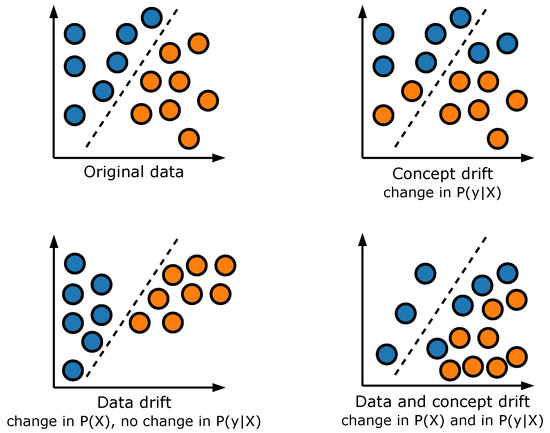
Figure 2.
Concept and data drifts. Figure adapted from [3,19].
When they occur, concept and data drifts can significantly affect the performance of machine learning models; thus, the challenge of online learning is to build algorithms that are capable of adapting to changes, even in real time. Several approaches have been developed in this area [6,7,8,9], with models that are trained per data instance which may also include drift detectors, such as the Adaptive Windowing (ADWIN) estimator [20]. These approaches are analyzed in the following paragraphs.
One of the earliest efforts that deals with evolving data streams and adapts to concept drifts is the Hoeffding Adaptive Tree model [6]. The algorithm builds a tree in an incremental way, and it uses a sliding window of variable length, which is changing over time, managing statistics at its nodes. The model has three different versions: HAT-INC, which uses a linear incremental estimator, HAT-EWMA, which uses an Exponential Weight Moving Average (EWMA), and HAT-ADWIN, which uses ADWIN for drift detection.
Other approaches have also adapted ensembles for the online learning scenario. For instance, Oza and Russell [21] designed an ensemble that uses the Poisson distribution to resample the data on which every base model is trained. Building on this approach, Bifet proposed the Leveraging Bagging method [7], an ensemble that further increases resampling by experimenting with larger Poisson lambda values. Moreover, the method uses random output detection codes instead of deterministic codes so that each classifier makes a prediction using a different function (rather than the same, which is standard practice in ensemble methods). And, finally, ADWIN is also used to detect concept drift; when changes are detected in the ensemble error rate, the base classifier with the highest error rate is replaced with a new one (model reset).
A similar approach is followed by Gomes [8], who proposed the Adaptive Random Forest method. This method also creates an ensemble model with decision trees as base learners, which are trained using Poisson distribution on resampling. The training process is based on the Hoeffding tree algorithm, with the main differences being that there is no early tree pruning and that whenever a node is created, a random subset of features is selected to decide the split at that point. This Adaptive Random Forest also uses a drift detection mechanism to cope with concept drift; the mechanism detects warnings of drifts, and when a warning occurs, a “background” tree is created and trained along with the ensemble without influencing the ensemble predictions. Then, if a drift is detected, the tree from which the warning signal originated is replaced by its respective background tree.
Another forest-based ensemble has been proposed by Rad et al. [10]. The authors introduced Hybrid Forest, a method using two components: a complete Hoeffding Tree as the main learner and many weak learners (also Hoeffding Trees) to improve prediction when needed. The main learner uses all data features, whereas each weak learner uses a subset of the features. The decision of whether the algorithm uses the main learner or the weak learners is based on the performance on the last samples, using a sliding window. When the number of correct answers of the weak learners is above a threshold (usually when drifts occur), their majority decision is used; otherwise, the main learner is used.
The Streaming Random Patches method [9] also creates an ensemble model, where the base models of the ensemble are decision trees (Hoeffding Trees). The trees are trained on data originating from resampling online bagging using the Poisson distribution. The main difference between this method and the Adaptive Random Forest is that random subsets of features are created in order to train every base model of the ensemble, thus achieving better diversity in models. Apart from that, Streaming Random Patches also integrates a drift detection method and adaptation similar to the Adaptive Random Forest.
An interesting combination of online ensemble methods is offered by the Performance-Weighted Probability Averaging Ensemble (PWPAE) [11]. The method uses two classification algorithms, Adaptive Random Forest and Streaming Random Patches, and combines them with two state-of-the-art drift detectors, ADWIN and DDM. A novelty of this method is that the weights of the ensemble models are not predefined; instead, they are modified dynamically according to the performance of each learner. PWPAE also employs k-means to sample the data in order to create a representative subset for the learning process.
The aforementioned approaches attempt to solve the problem of the occurrence of drifts in evolving data streams; however, their main drawback is the requirement of manual configuration. Moreover, those algorithms may be effective on certain data streams, but they do not generalize well to others due to the fact that they are limited by the specifics of each classification algorithm. As a result, recently, several researchers have attempted to design AutoML approaches for evolving data streams [12,13,15,16,17]. AutoML is a field of machine learning that aspires to automate model selection and hyperparameter optimization, thus providing a configuration that is effective on a variety of data. In the context of online learning, AutoML models are typically coupled with drift detection mechanisms.
One such solution is the adaptation algorithm proposed by Madrid et al. [12]. The authors implemented a modification to the Auto-Sklearn machine learning toolkit [22], which integrates countermeasure mechanisms for concept drifts in data streams. The method receives data in batches. The first batch is used to train the first ensemble model using Auto-Sklearn. This ensemble model is then used to make predictions on the next batch, and subsequently, when the real values arrive, a Hoeffding Drift Detection Method (FHDDM) [23] is used to determine whether there is any concept drift in the data. If there is, the model is updated, either via full model replacement (a new model is created and trained with the data of all past batches) or by changing the weights of the ensemble (using the latest batch or all the stored batches).
Another approach is EvoAutoML [13], an AutoML method that expands on online bagging [21], inspired by genetic algorithms. The method initially creates an ensemble with a random population of algorithm pipelines. After that, the algorithm decides when a mutation should occur in this population, based on a sampling rate. When a mutation is about to happen, the algorithm chooses the best pipeline and changes a random parameter to create the new pipeline, while also determining the worst pipeline, in order to be removed from the population. After the mutation step, the population is trained on the new instance (every sample).
Another AutoML approach that is also based on evolutionary algorithm generation is AutoClass [14]. Initially, AutoClass creates a population of algorithms with their default parameters (Hoeffding Tree, Hoeffding Adaptive Tree, kNN with and without ADWIN). After that, a sliding window is used to decide each time which configuration should been removed, and which should be added with new parameters. The decision is made using fitness proportionate selection [24], where the fitness of each configuration is defined as its predictive performance.
An alternative approach is followed by Chacha [15], an AutoML method that is used to determine the best parameters for the prediction model. Upon setting up the initial configuration, the algorithm continuously determines the best configuration as the data are coming. The best configuration (champion) is determined each time by comparing the latest best one with others from memory (challengers) based on the value of the progressive validation loss metric. The challengers are limited to a number provided by the user, while not all challengers run (and compete with the champion) at the same time for efficiency. Every time a new sample arrives, it is used by the champion for prediction, and after that (when the real value arrives), it is used to update the champion and some of the challengers (the live models). Subsequently, the algorithm chooses if it needs to change the champion or to remove any model from the challengers (and replace it with a new one).
ASML [17] is an online AutoML method, which further focuses on providing a scalable solution by creating simple pipelines or ensembles (depending on user configuration). A batch of data is needed at the beginning to train the initial pipelines and determine the optimal one. After that, every time a new batch of data arrives, it is used to assess a set of different pipelines. Apart from the best pipeline at the time, the pipelines to be assessed are generated from adaptive random directed nearby search, and from random combinations of the search space.
A similar approach is followed by the OAML method [16]. OAML initially requires an amount of data to train a number of different pipelines, then evaluate them in order to find the best one to use. Every time a new instance arrives, it is initially used for prediction and subsequently (when the real value arrives) for training the pipelines. The method further involves an Early Drift Detection Method (EDDM) [25], which is used to detect concept drifts. Every time a drift is detected or a set number of samples arrives without the model having been replaced, the method initiates a retraining phase, where it takes the same steps as in the first training, using the samples in memory.
Although the aforementioned approaches are effective under specific scenarios, they also have certain limitations. First of all, the approaches that do not employ drift detection methods may not be a good fit for data streams with abrupt changes in the distribution of the data, as they might only adapt to gradual drifts. Other approaches focus only on concept drifts, not adapting the models preemptively in the case of data drifts. Concerning adaptability, online machine learning methods may need manual configuration to optimize their parameters. In contrast, AutoML methods are optimized automatically, although they often lack preprocessing algorithms, and they are sometimes limited by the types of classification models used (e.g., some support only one category of classification models and are thus mainly focus on hyperparameter optimization). Moreover, certain approaches have to wait for multiple batches of data to arrive before initialization, as they base their retraining on large time windows. Finally, certain implementations are not available online and/or do not employ state-of-the-practice libraries.
In this work, we design an AutoML algorithm that overcomes all of the above limitations. Table 1 summarizes certain features of the methods analyzed above while also including the advantages of our method in these aspects. As shown in this comparison, our method supports both concept drift and data drift detection using the ADWIN algorithm. In contrast, all other approaches focus only on concept drifts, while certain AutoML implementations do not even explicitly include a drift detector [13,14,15,17]. Instead, they are based only on the online adaptation capabilities of the underlying models, which may hinder their effectiveness on sudden drifts. Another important distinction is whether the proposed solutions also include data preparation steps, i.e., if they offer end-to-end pipelines.

Table 1.
Comparison of methods used on data streams.
As shown in Table 1, there are several approaches that only offer classification models [6,7,8,9,10,11,14,15]; thus, they require significant effort by the user to preprocess the data and possibly perform feature selection. Even AutoML approaches are usually limited only to preprocessing methods [12,13,16], whereas ASML [17] and our proposed approach (AML4S) are the only ones that further support feature selection. As a result, AML4S does not require any knowledge of data or any machine learning expertise, as it identifies the optimal algorithms and parameters for each pipeline step (preprocessing, feature selection, model selection, hyperparameter optimization) automatically.
Furthermore, concerning the search space of each method, we note that AutoML methods are obviously expected to be more effective than single classifiers, especially when they support a large variety of online classification algorithms, with multiple configurations. In this aspect, both the Adaptation algorithm of Madrid et al. [12] and AML4S are quite effective, as they support 15 and 12 models, respectively (including different categories of models, as discussed in Section 3.2). However, the Adaptation algorithm is more oriented towards efficient AutoML, which is expected, as it employs the Auto-Sklearn library [22], whereas our approach focuses on the challenges of online learning to a great extent, as well. More specifically, after initialization, our method is fully online, as it is trained per instance and not in batches, while it also performs retraining only upon drift detection (thus not requiring a configurable time parameter). Finally, our pipeline is implemented using River [26], which is a state-of-the-practice online machine learning library, facilitating the application of our approach to different problems in a straightforward manner.
3. Materials and Methods
3.1. Overview
The architecture of AML4S is shown in Figure 3. The main module of AML4S is a pipeline that is used for predictions. This pipeline contains a preprocessor, a feature selector, and a classifier. Our method also has a drift detector, used for detecting concept and data drifts, as well as an AutoML pipeline selector, which chooses the best pipeline for prediction at initialization and after every confirmed drift detection.
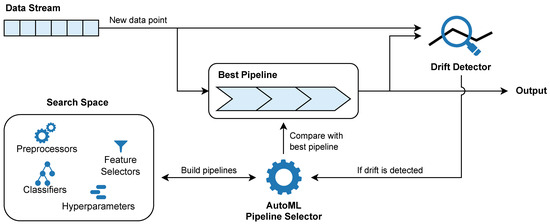
Figure 3.
Overview of AML4S.
More specifically, at initialization, AML4S creates a sliding (memory) window to hold the streaming data and utilizes the first data to arrive in order to build a set of different pipelines. The possible configurations are defined by the search space, while the AutoML pipeline selector determines the best pipeline based on the input data. After that, the best pipeline continuously makes predictions on new instances while evolving at the same time by training on them. The data input and the validity of the prediction are also continuously forwarded to the drift detector, which detects data drifts as changes to input features’ distributions, as well as concept drifts as changes to the accuracy of the model. When a new concept drift or data drift is detected, the drift detection mechanism of AML4S notifies the AutoML pipeline selector in order to rebuild the pipelines and compare them with the currently selected pipeline (best pipeline). The optimal pipeline then takes the place of the best pipeline and becomes the new best pipeline.
As already noted, the implementation of AML4S employs the online machine learning library River [26], which provides a straightforward interface for building online algorithms. Each data instance is initially used for prediction (testing), and after that, it is immediately used for algorithm training. Thus, AML4S can handle different types of shifts in the data distributions. As an online method, it can effectively adapt to evolving data, therefore effectively responding to gradual or incremental changes in the features (data drifts) and/or the target variable (concept drifts) of the data stream (see Figure 1). At the same time, AML4S can also handle sudden drifts, since its drift detection capabilities can identify abrupt anomalies, thus adapting to them.
In fact, our method closely follows the principles and the API conventions of River as a means to facilitate the practical application of AML4S in real-world settings. More specifically, the AML4S interface is modeled after the River API calls predict_one and learn_one, which enable using a data instance for prediction and then using it for training, respectively. These functions receive as input both the features and the target value of the data instance in order to enable training and evaluation of the effectiveness of the algorithm. Moreover, similarly to the River API, all other parameters are set during initialization (buffer size, use of concept/data drift detector, search space). The repository of our implementation, which can be found at https://github.com/AuthEceSoftEng/automl-data-streams (accessed on 22 August 2025), further includes specific instructions for applying our approach to data stream settings.
The modules of AML4S are analyzed in detail in the rest of this section. In Section 3.2, we analyze the pipeline module, which includes the preprocessor, feature selector, and classifier components (with different hyperparameters), while in Section 3.3, we analyze the drift detection mechanism and the AutoML pipeline selector.
3.2. AutoML Pipeline
As already mentioned, the search space used to build the different pipelines of AML4S consists of preprocessors, feature selectors, and classifiers, along with their hyperparameters. For the preprocessor, we define the following three options:
- None, without any kind of preprocessing,
- StandardScaler, which scales the data so that it has zero mean and unit variance, and
- MinMaxScaler, which scales the data to a fixed range from 0 to 1.
The different options for the feature selector are:
- None, without any kind of feature selection,
- VarianceThreshold, which removes low-variance features, and
- SelectKBest (similarity=stats.PearsonCorr(), k=3), which removes all but the three highest-scoring features based on the Pearson correlation coefficient.
Finally, for the classifier component, our method involves the options shown in Table 2. As shown in this table, the provided classifiers span multiple categories of algorithms. Specifically, the list includes statistical models (e.g., logistic regression), probabilistic classifiers (e.g., Gaussian Naïve Bayes), forests (e.g., Hoeffding Tree), instance-based models (e.g., KNN) and even ensembles (e.g., Adaptive Random Forest). Diversity in the types of the models is quite important, as different models may be effective on different data distributions, thus enhancing the versatility and robustness of our system. Specifically, Logistic Regression is effective on linearly separable problems while also providing fast updates. However, it may struggle in cases of non-linear data distributions. At the same time, the probabilistic nature of Naïve Bayes makes it an intuitive fit for data streams, as its probability estimates are already updated incrementally, and the algorithm is computationally efficient. Furthermore, it performs reasonably well in cases of missing values and high-dimensional and/or sparse data.
Table 2.
Classification algorithms of AML4S, including their parameters and search spaces.
Hoeffding trees and their variants were chosen due to their inherent suitability for streaming data and their adaptability to rapid distribution changes, while ensemble models are also included, as they enhance the effectiveness of trees by constantly replacing underperforming models, also effectively adjusting to evolving distributions. Lastly, KNN was selected due to its natural adaptability to drifting, as its predictions are based on recent instances, as well as its versatility to a wide range of data streaming scenarios, since it does not assume any prior data distribution. However, it is computationally expensive and may struggle in high-dimensional data, hence making it preferable for low-velocity streams. Finally, we note that for each model, we define a hyperparameter default search space (shown in the last column of Table 2), constructed of values that are either River’s defaults or are commonly used with their respective algorithm. Through the use of grid search for hyperparameter tuning, we found the chosen ranges to provide adequate pipeline diversity and performance in most cases, since they allow for hyperparameter combinations that are well-suited for rapid adaptation (e.g., lower grace period values), as well as noise resilience and stability (e.g., higher number or neighbors), while also managing computational costs (e.g., number of neighbors/tree estimators) (see Section 4).
In total, for this default configuration of AML4S, our search space includes 657 pipeline combinations (3 preprocessing choices × 3 feature selection choices × 73 classifiers with different parameters). Note that these choices are merely indicative examples of the capabilities of our approach and were mainly selected for their simplicity and broad applicability. Since our pipeline and overall methodology is based on the standard interface of the River framework [26], it is straightforward to add more algorithms and configurations or to remove ones that may be redundant in certain use cases. For all pipelines that are instantiated (see Section 3.3), the interface includes two methods, one for predicting the target output of new instances (predict_one) and one for training the components (learn_one).
3.3. Drift Adaptation
Our method adapts to streaming data in two ways. First and foremost, as already mentioned, AML4S is an online learning system, where every sample that is used for prediction is also used for training after the ground truth value of the target variable becomes known. This is very useful for small changes in the data distribution and occurs automatically given the online nature of the algorithm; however, it does not account for abrupt drifts. Hence, we introduce the second method of adaptation: a drift detection mechanism. When a substantial distribution shift occurs either on the input data stream or the output of the model, AML4S identifies it as a drift and updates its pipeline to ensure continuous and effective predictions.
In order for AML4S to identify both concept drifts and data drifts, we create a detector consisting of two components: one for concept drift detection and one for data drift detection. Since the focus of this work is not drift detection explicitly, but rather providing a unified, online AutoML solution, both parts employ ADWIN [20], a drift detection algorithm that is well-established, highly adaptive, and can detect different types of drifts such as those indicated in Figure 1. Contemporary research has shown that it can be effective both for data and for concept drifts [27,28]. The algorithm relies on a variable-length sliding window w, which continuously consumes the arriving data instances. ADWIN then splits the window into two consecutive sub-windows, and . An example binary concept scenario is shown in Figure 4.
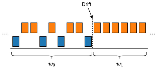
Figure 4.
Example depicting the sub-windows of the sliding window of ADWIN when a drift is detected.
Given the data instances (or the error values in case of concept drift) of the two sub-windows, ADWIN computes the average value for each window. If the absolute difference between the two average values is higher than a significance threshold, then ADWIN detects a drift. The detection of a drift is formally defined as follows:
where and are the average values of the sliding windows and , respectively, and is the value of the significance threshold, calculated based on Hoeffding’s inequality [20]. Therefore, is automatically computed as new data arrives, and it varies according to the number of elements in each sub-window and the confidence parameter , which is configurable and controls the detector’s sensitivity. Higher values of result in smaller values of , which make ADWIN more sensitive to distribution fluctuations but may increase false positives. On the other hand, lower values of , and hence higher values of , result in a stricter detector that may miss actual drift occurrences. Furthermore, its statistical nature also makes the model resistant to isolated outliers, as they rarely cause a persistent shift in the mean of a sliding window.
Using ADWIN, we build two components for the drift detector of AML4S, shown in Figure 5. The first component, which is the data drift detection component, receives the data instances X as input. For each individual feature , it applies an independent ADWIN sliding window to monitor fluctuations in the feature’s distribution, effectively performing univariate data drift detection. To enhance resistance against false positive detections, rather than relying on a fixed percentage of drifting features to signal a drift, our method is more conservative and model-aware; specifically, a distribution shift is considered as an actual data drift only if the following conditions are met:
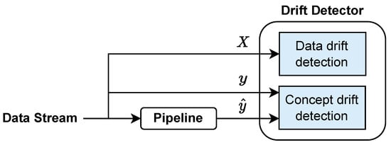
Figure 5.
Components of the drift detector of AML4S.
- a data drift has been detected by ADWIN,
- no recent concept drift has been detected, and
- the model’s prediction accuracy, measured over a sliding window, drops by more than a predefined threshold (in our case, 7%).
This combined approach allows the system to detect actionable data drifts that are both statistically evident and impactful to the model’s performance. The second component is responsible for concept drift detection, as it monitors the accuracy of our model. Specifically, as soon as our pipeline makes a prediction, , and the ground truth, y, is known, the error between the two values, , is passed as input into another ADWIN sliding window. Contrary to data drifts, changes in this distribution are always considered meaningful.
If either a data or a concept drift are verified, we discard the data preceding the point of the drift and store new data in memory until we reach a sufficient amount to train new instances of AutoML pipelines. By conducting internal tests regarding the memory size, we decided on 450 samples to ensure sufficient recent context for drift detection and performance evaluation while avoiding high memory and computational overhead. Additionally, this practice also reinforces robustness against extreme outlier cases, as newer incoming data will minimize outlier impact, effectively filtering it out. If the distance from the detected drift is greater than our memory size, then we keep the latest samples until the memory is full, effectively maintaining a sliding window of the 450 most recent data points at all times.
Thus, either upon initial deployment or at drift detection, the AutoML pipeline selector performs the steps shown in Figure 6. First, every possible pipeline is created through combinations of the algorithms in Section 3.2. The pipelines are then trained and evaluated using the data from memory to determine the pipeline with the highest accuracy; if multiple pipelines are equally accurate, we randomly choose one of them. Finally, in the case of detected drift (since a pipeline is already deployed), we compare the selected pipeline with the currently used (previously best) pipeline and choose the one with the highest accuracy between the two.
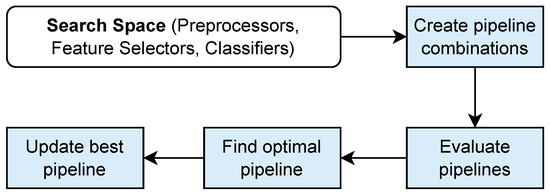
Figure 6.
Steps of the AutoML pipeline selector of AML4S.
4. Results
We evaluate our method against online learning algorithms, as well as a state-of-the-art online AutoML implementation. Our comparison with the rest of the online learning algorithms involves various data streams, both synthetic and real. Section 4.1 provides details about the synthetic data streams, which were generated using a data generator of our making, while Section 4.2 presents the results of our evaluation on different synthetic and real data streams. Finally, the results of the evaluation of our approach against a state-of-the-art online AutoML methodology are presented in Section 4.3.
4.1. Synthetic Data Generator
For the evaluation of the proposed method, we extended the loan data stream generator described by Agrawal [29]. The generator concerns a scenario of applicant profiling for receiving a loan to buy a house. It involves eight features (salary, commission, age, education level, zip code, house value, loan years, loan), denoting different attributes of the customer application, as well as a class variable signifying whether the loan application is accepted. These features are described in Table 3.
Table 3.
Variables of the Loan data generator.
Concerning the target variable, our generator allows for multiple options regarding the number of classes. Specifically, we define the following options:
- 2 classes: the loan application is either Approved or Declined.
- 3 classes: the loan application has three states, i.e., Approved, Conditionally Approved, and Declined.
- 4 classes: the loan application has four states, i.e., Approved, Conditionally Approved, Exceptionally Declined, and Declined.
Finally, the most important feature of our generator (and, practically, the reason we developed it) is that one can add different types of drifts in the data. Specifically, the generator allows for adding both concept drifts and data drifts at any position, as well as setting the type of the desired drift (as shown in Figure 1). To do so, we design a financial scenario that allows for three states: crisis, normal, and growth (the scenario is of course fully synthetic, as is all the dataset, and its purpose is not to accurately describe loan applications with respect to different financial settings, but rather to provide a testbed for drifts). For data drifts, these states are reflected by the salary variable. For the normal state, the salary (as also mentioned in Table 3) is uniformly distributed in the range . For the crisis state, the salary distribution is in the range , while for the growth state, the salary distribution is in the range .
Concerning concept drifts, the changes in the financial states are reflected in the classification function; a practice also followed in [29]. For instance, when there are two classes (Approved and Declined), in order for a loan to be approved in the crisis state, the amount of the loan has to be lower than or equal to 10 times the salary of the applicant, and at the same time, it must not exceed half of the value of the house. In the growth state, however, one can have their loan approved even if the amount asked is 10% of the house value. The conditions for all financial states and all scenarios (2, 3, or 4 classes) are described in full detail in Appendix A.
For our evaluation, we created three data streams: one with 2 classes, one with 3 classes, and one with 4 classes, with 20,000 samples each. In every data stream, we placed both concept and data drifts, as described in Table 4. As shown in this table, in order to account for different cases, we also added co-occurring data and concept drifts (e.g., in the 6000th data point or the 16,000th data point).
Table 4.
Concept and data drift positions for our evaluation set.
Figure 7 provides a visualization of the dataset for a scenario of 2 classes, including the drifts defined in Table 4. The diagram depicts 20,000 data instances, including all features, as well as the target variable (y). Concept drifts are noted with a dashed line, while data drifts are noted with a dotted line. It is interesting to note that the distribution of salary indeed changes when a data drift occurs.
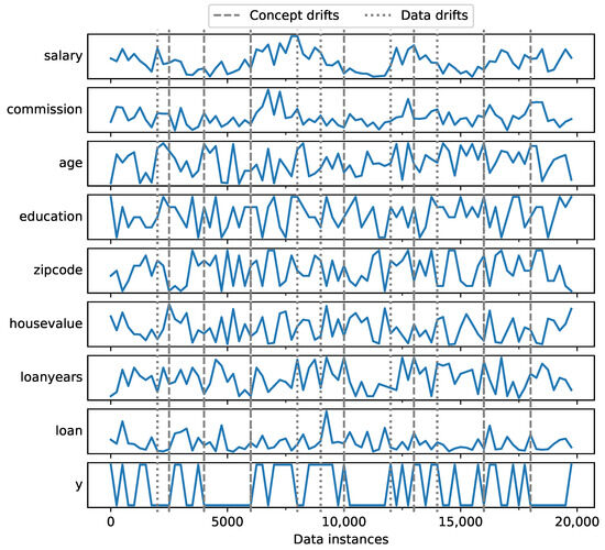
Figure 7.
Loan dataset instances including concept and data drifts.
Concerning the target variable, we observe that it is affected both by concept drifts and data drifts. For example, the crisis that occurs at the 4000th data instance, indicating a concept drift, seems to severely influence loan application approval, as all loans are now rejected until the distribution switches to growth (6000th instance). An example of data drift that has a similar effect is shown in the 9000th instance; a crisis that results in lower salaries seems to also affect the target variable, as fewer loans are approved, even if the classification function itself does not change (i.e., the criteria for loan approval remain the same).
4.2. Comparison with Online Models
4.2.1. Comparison with Synthetic Data
To ensure that AML4S is effective, we compare it with several state-of-the-art online models provided by the River framework [26], specifically with Hoeffding Adaptive Tree, Hoeffding Tree, Logistic Regression, and the Aggregated Mondrian Forest (AMF) Classifier. These algorithms were chosen because they provide coverage on a plethora of learning criteria; Logistic Regression is a linear model, functioning as a baseline. Hoeffding Tree and the AMF Classifier are based on online tree and forest implementations, respectively, which are known to be effective for online learning. Hoeffding Adaptive Tree is an adaptive method that further integrates an ADWIN drift detector; hence, it shall provide an interesting comparison to our pipeline. Finally, these models were also evaluated in conjunction with the Standard Scaler provided by River to further assess the effect of preprocessing.
We conducted three experiments, one for each dataset of Section 4.1 (2 classes, 3 classes, 4 classes), while always using a memory of 450 samples. To make the comparison as comprehensive as possible, we employ the accuracy metric. However, since we are comparing online models, we compute what we may call the model’s moving accuracy, i.e., the accuracy of the last 100 instances, and the moving average accuracy, i.e., the aggregated accuracy of the model from the start to a certain data instance. The results for the binary classification problem are shown in Figure 8. Figure 8a depicts the moving accuracy of AML4S, including the different types of drifts. Interestingly, we may note how our method is quick to adapt to drifts, as its accuracy quickly recovers (within a few data instances, enough to train the new pipelines of AML4S), even after feature distribution shifts.
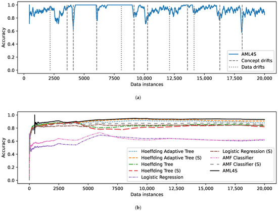
Figure 8.
Evaluation results on the loan dataset for 2 classes, including (a) Accuracy of AML4S and different drifts of the loan dataset for 2 classes. (b) Moving average accuracy of AML4S versus different online methods on the loan dataset for 2 classes.
The comparison of AML4S versus the rest of the online methods is shown in Figure 8b. In this diagram, one may clearly observe the need for drift detection algorithms. Specifically, both our method and the Hoeffding Adaptive Tree seem to outperform all other methods. This indicates that ADWIN is effective for detecting drifts; therefore, pipelines that include it can adapt to changes in the distribution of the data and maintain high accuracy levels. Concerning preprocessing, using scaling seems to lead to better results, which is evident since the Hoeffding Adaptive Tree with Standard Scaler pipeline (Hoeffding Adaptive Tree (S)) outperforms the Hoeffding Adaptive Tree without any scaling. Moreover, we see that AML4S is more effective than the Hoeffding Adaptive Tree pipeline, indicating that detecting both data drifts and concept drifts is optimal in this case.
For the second experiment, we make the problem more challenging by introducing a third class in our synthetic dataset, the results of which are shown in Figure 9. As one may see, in Figure 9b, AML4S is again more effective than all other algorithms, indicating that it is robust, even on multi-class problems that pose a challenge to most models. Specifically, concerning the other algorithms, we may note that the tree implementations seem to have higher accuracy than Logistic Regression, which is expected given the linear nature of the latter. The AMF Classifier, on the other hand, seems to be sensitive to features of different ranges, as using the Standard Scaler significantly improves the accuracy of the algorithm.
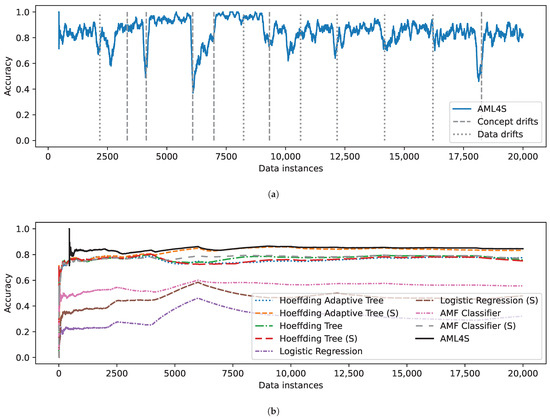
Figure 9.
Evaluation results on the loan dataset for 3 classes, including (a) Accuracy of AML4S and different drifts of the loan dataset for 3 classes. (b) Moving average accuracy of AML4S versus different online methods on the loan dataset for 3 classes.
Concerning the drift adaptation capabilities of our algorithm in the case of 3 classes (Figure 9a), it is again clear that it quickly returns to high accuracy values after retraining, i.e., when detecting concept or data drifts. This indicates that the drift detection mechanism of AML4S is effective for drift detection, allowing our method to train improved pipelines.
Similar observations can be made for the data stream scenario with 4 classes, the results of which are shown in Figure 10. In this case, it is clear that the scenario is much more challenging, for all models. For instance, as shown in Figure 10b, the performance of Logistic Regression is comparable to random classification, while the algorithm predicts the true class no more than half of the time, even with scaling. And although the accuracy of tree-based algorithms is higher, AML4S is still clearly most effective in this scenario.
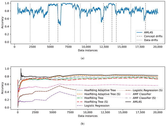
Figure 10.
Evaluation results on the loan dataset for 4 classes, including (a) Accuracy of AML4S and different drifts of the loan dataset for 4 classes. (b) Moving average accuracy of AML4S versus different online methods on the loan dataset for 4 classes.
As in the previous scenarios, AML4S handles the different drifts effectively (shown in Figure 10a). Concerning concept drifts, once again, we observe that the accuracy of AML4S drops when retraining occurs. However, in most cases, it rises quickly to the previous value. The behavior of AML4S for data drifts is also satisfactory; in certain drifts (such as in the 2000th or in the 14,000th instance), the accuracy of the method does not drop at all. Finally, in instances where the two drift types co-occur (such as the 6000th or the 16,000th instance), AML4S again quickly ‘rebounds’ to high accuracy values.
Overall, it seems that AML4S consistently outperforms all other methods in the different scenarios of the loan data stream. This is shown in Table 5, which summarizes our findings for this comparison, presenting the accuracy for all settings and algorithms. Moreover, the second best algorithm is consistently the Hoeffding Adaptive Tree implementation coupled with the Standard Scaler. This is more or less expected, since this is the only other algorithm that includes a drift detector and a preprocessor. Another interesting note is that using the Standard Scaler is overall more effective; this is the case for all four algorithms that were chosen for the purpose of these experiments. In certain methods, such as Logistic Regression or the AMF Classifier, the increase in accuracy when using scaling is quite significant, as these models tend to be more sensitive to varying data ranges. Tree-based implementations, on the other hand, are more robust in such scenarios. In any case, as AML4S includes all these algorithms in its pipelines, it is reasonable to assume that it can perform better in most scenarios, a conclusion also justified by our findings.
Table 5.
Accuracy of AML4S versus online methods on the loan dataset for 2, 3, and 4 classes (highest values highlighted using bold typeface).
Finally, in Table 6, we provide the data points at which our drift detector has detected different types of drifts, along with the actual (ground truth) drifts for the 3 dataset configurations. The detection results confirm that ADWIN is effective for detecting both concept and data drifts, while most drifts are detected only a few instances away from their actual position. Therefore, the drift detector is efficient for updating the pipeline. Moreover, one may see that there is only one false positive case as well as only two cases of non-detected drifts (false negatives). The algorithm also correctly classifies most drifts into concept and data ones, slightly favoring concept drifts when both types co-exist.
Table 6.
Concept and data drift positions for our evaluation set and detected positions.
4.2.2. Comparison on Real Data
To further evaluate our method against online learning algorithms and assess its applicability to real-world scenarios, we also use two real datasets: the Covtype dataset [30] and the Rialto dataset [31]. The Covtype dataset contains tree observations from four areas of the Roosevelt National Forest in Colorado. The purpose of this dataset is to predict the dominant species (cover type) of the tree in a forest (among 7 different species) given 54 features of each area, most of them cartographical. All of the areas have minimal human intervention, so the observations are related to ecological processes. The total number of observations exceeds 581k, while the data are provided as a stream that involves multiple concept drifts. The Rialto dataset is a data stream about image classification, so it would be interesting for us to see how our algorithm works on such tasks. It contains 27 features, derived from the encoding of images in a normalized 27-dimensional RGB histogram. Those images were obtained from time lapse captures of a fixed webcam with the purpose of identifying a specific building in the picture among 10 different buildings. The varying weather conditions introduce noise and make classification more challenging.
Figure 11 depicts the evaluation results for the Covtype data stream. As shown in Figure 11a, AML4S detects the concept drifts that occur throughout the stream and effectively models them, therefore achieving high accuracy until the end of the experiment. In Figure 11b, we can see that our method achieves the highest accuracy among the rest of the online learning methods. Interestingly, in this dataset, it seems that the AMF classifier outperforms the adaptive tree pipelines (Hoeffding Adaptive Tree with/without Scaling), possibly due to the complexity of this dataset. Covtype includes 54 features and 7 different classes; thus, it would possibly be a good fit for methods with multiple parameters (like the forests of AMF). Moreover, we once again see how the choice of classifier can have a significant impact on the results; for example, logistic regression falls below 40% accuracy.
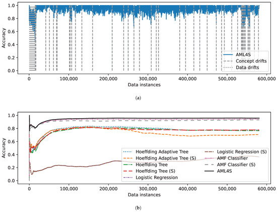
Figure 11.
Evaluation results on the Covtype dataset, including (a) Accuracy of AML4S and different drifts of the Covtype dataset. (b) Moving average accuracy of AML4S versus different online methods on the Covtype dataset.
Concerning Rialto (Figure 12), our method detects several concept and data drifts, shown in Figure 12a. Due to the noisy nature of the data, it is expected that multiple distribution shifts may occur in the 27 histogram-extracted features. These shifts are very often interpreted as data drifts by AML4S, which, however, does not undermine the effectiveness of our algorithm. In fact, it seems that the AutoML pipeline selector often does not replace the best/selected pipeline as a response to the data drift, therefore indicating that the detected drifts are subtle and do not affect the performance of our algorithm. In the comparison with the other online methods (Figure 12b), our method again outperforms all other algorithms, although by a small margin in comparison with the two variants of the AMF classifier, indicating, possibly once again, the complexity of the data variables.
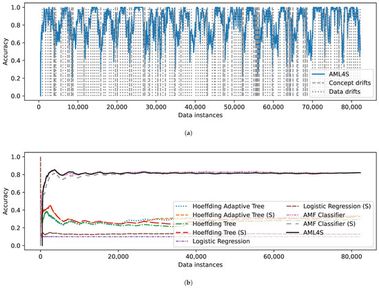
Figure 12.
Evaluation results on the Rialto dataset, including (a) Accuracy of AML4S and different drifts of the Rialto dataset. (b) Moving average accuracy of AML4S versus different online methods on the Rialto dataset.
The results of comparing AML4S to online learning algorithms on the real data streams are summarized in Table 7. Overall, it seems that AML4S is also quite effective in these real-world scenarios. It manages to achieve high accuracy on data streams of high dimensionality that also exhibit different type of drifts, as well as multi-class scenarios, despite the fact that it does not incorporate mechanisms to handle class imbalance. Interestingly, the AMF classifier is the second best method in both experiments, indicating that ensembles are robust choices when it comes to data streams with large/complex feature space.
Table 7.
Accuracy of AML4S versus online methods on real datasets (highest values highlighted using bold typeface).
Table 8 further depicts the average time required for our online methodology to process an instance (Mean Processing Time) and the average time required to train all pipelines (Mean Retraining Time). The experiments were run on a system with an AMD Ryzen 7 5700G processor and 32 GBs of RAM (although most of it was not used, as the task was CPU-bound). Concerning the loan dataset, note that in all three cases, the time required to process an instance is roughly one hundredth of a second. Moreover, in cases where a drift is found, full pipeline rebuilding (by training and evaluating all pipelines) requires roughly 15 s. The results for the real datasets are similar; Rialto requires roughly one twentieth of a second for processing one data instance, while the full pipeline can be retained in slightly more than 25 s. The corresponding values for Covtype are roughly 0.05 s and 23 s, respectively. Thus, all of these cases indicate that AML4S could be used in a real-time setting.
Table 8.
Mean processing and retraining times of AML4S on synthetic and real datasets.
Finally, to further validate the results of our evaluation against online algorithms, we performed a Wilcoxon signed rank test [32] to determine whether the higher accuracy of our method compared to that of the other algorithms is statistically significant. We applied the one-tailed test twice, once for the Hoeffding Adaptive Tree and once for the AMF Classifier (both algorithms with scaling), as these two algorithms are the closest to AML4S in terms of accuracy. Specifically, the mean accuracy of AML4S over all five cases (three of the synthetic dataset generator and two of the real data streams) is 0.88 (median 0.85), while the same values for Hoeffding Adaptive Tree and the AMF Classifier are 0.71 and 0.83, respectively (medians of 0.79 and 0.82, respectively). In both cases, the Wilcoxon z statistic value is and the null hypothesis (that these algorithms have equal accuracy to ours or even higher) is rejected with a p-value of , meaning that the accuracy values of AML4S are significantly higher than those of the Hoeffding Adaptive Tree or the AMF Classifier at .
4.3. Comparison with OAML
The second type of experiment we performed was a comparison with the OAML method [16]; in particular, with OAML-basic, which is very similar to our approach, as mentioned in Section 2. While there is partial overlap in the classifiers used by AML4S and OAML-basic, such as Hoeffding Trees, Logistic Regression, Perceptron, KNN, and Adaptive Random Forests, our method employs most of those as standalone classifiers, while OAML integrates them in its ensemble models. Hence, AML4S extends the search space by including additional diverse models suitable for different kinds of settings, as seen in Table 2. Furthermore, unlike OAML-basic, which only addresses concept drift via EDDM and retrains periodically or upon drift, our method detects and distinguishes both concept and data drifts though the ADWIN drift detector and triggers retraining only when necessary, based on performance impact. This leads to more efficient adaptation. Given that the implementation of the method is not available online, we compared our system with OAML-basic on four data streams used by the authors of the method. Specifically, we use the following data streams:
- Electricity [33]: The Electricity dataset contains price data for the electricity of the Australian New South Wales market. It includes 7 features (e.g., electricity demand and electricity price values) and around 45k instances. The goal is to predict whether the price increases or decreases (binary classification). The dataset is highly volatile with gradual drifts, as its price values are set every five minutes and are constantly affected by supply and demand. Moreover, the data may be biased by electricity transfers to/from the neighboring state of Victoria (used to avoid electricity fluctuations); thus, the relevant variables are also added to the dataset.
- Vehicle [34]: The Vehicle dataset contains data from the sensors of a wireless network of vehicles. It includes 100 features and around 100k instances. The goal is to classify the vehicles into four classes (multi-class classification). The collected data variables in this case may include significant noise; therefore, this dataset is a suitable benchmark for assessing the robustness of the methods against noisy data.
- Airlines [35]: The Airlines dataset contains information about flights (and their schedules). It includes 9 features (e.g., departure data, time of flight, etc.) and around 500k instances. The goal is to predict whether the flight arrived on time or there was a delay (binary classification). The dataset involves 100 concept drifts, which are expected to influence the performance of the algorithms.
- Hyperplane [36]: The Hyperplane dataset contains data generated using a rotating hyperplane. The synthetic data stream used by OAML includes 10 features and 500k instances. The goal is to classify data points as above (positive) or below (negative) the hyperplane (binary classification). From an evaluation perspective, this dataset can be mainly used to assess gradual drifts, especially with respect to the noise resilience of the methods (the data include 5% label noise).
The results of the comparison with the Electricity data stream are shown in Figure 13. Figure 13b depicts the moving average accuracy of OAML-basic versus two configurations of our pipeline: one detecting only concept drifts (AML4S-CD) and one detecting both concept and data drifts (AML4S). Note that while AML4S uses 450 instances for its memory, OAML uses 5000 instances. The results clearly indicate that AML4S outperforms OAML in this data stream.
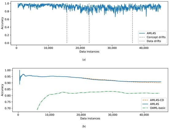
Figure 13.
Evaluation results of AML4S versus OAML-basic on the Electricity dataset, including (a) Accuracy of AML4S and different drifts of the Electricity dataset. (b) Moving average accuracy of AML4S versus OAML-basic on the Electricity dataset.
The accuracy of both of our configurations is similar, which is expected since the Electricity dataset does not include any data drifts. Indeed, as shown in Figure 13a, AML4S effectively detects shifts in the relationship between inputs and outputs and maintains high accuracy throughout all instances.
Figure 14 presents the performance of the systems on the Vehicle data stream. Interestingly, in this case, we see how AML4S detects certain data drifts (Figure 14a). By examining them manually, we found that these are, in fact, co-occurring data and concept drifts, which is expected given the nature of the dataset. Sensor data are typically sensitive and can introduce data distribution changes for multiple reasons (e.g., noise from interference, sensor malfunction, etc.). These changes, in turn, are reflected to the target variable, therefore introducing possible concept drifts. Our method seems to effectively detect these drifts, as its accuracy does not drop significantly at any point during the classification of the data stream.
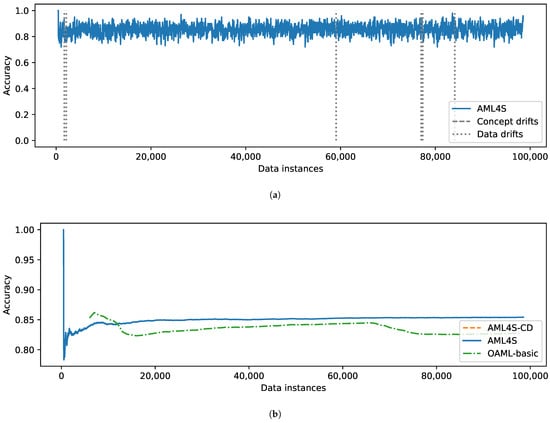
Figure 14.
Evaluation results of AML4S versus OAML-basic on the Vehicle dataset, including (a) Accuracy of AML4S and different drifts of the Vehicle dataset. (b) Moving average accuracy of AML4S versus OAML-basic on the Vehicle dataset.
The comparison with OAML-basic, which is shown in Figure 14b, indicates again that our method is more effective. Another interesting observation here is that AML4S also seems more robust in cases where the data distribution shifts; specifically, we observe how the accuracy of OAML-basic drops after 70,000 instances, possibly due to a change in data distribution, and never recovers. Conversely, the two AML4S implementations do not seem to be affected by the same change.
The results for the Airlines data stream are shown in Figure 15. In this case, the results are quite interesting, given that the data distribution of this data stream involves several changes. As shown in Figure 15a, AML4S identifies more than 50 concept drifts and manages to handle them effectively, as its accuracy drops only for a few instances before rising back to prior levels.
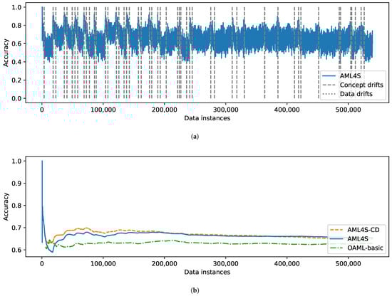
Figure 15.
Evaluation results of AML4S versus OAML-basic on the Airlines dataset, including (a) Accuracy of AML4S and different drifts of the Airlines dataset. (b) Moving average accuracy of AML4S versus OAML-basic on the Airlines dataset.
The comparison of the algorithms, shown in Figure 15b, once again illustrates that AML4S outperforms OAML-basic. Interestingly, in this case, the version of AML4S that only involves concept drift detection (AML4S-CD) seems to achieve higher accuracy than the version that handles both types of drifts (AML4S) during the first instances. This is possibly due to the fact that the Airlines dataset includes several concept drifts that are not necessarily related to data features. For example, a flight could possibly be delayed for unforeseen circumstances, such as weather events, which are not included as features of the dataset. Instead, the dataset includes features like flight numbers, distance, destination, etc., which are not often subject to changes in distributions.
Finally, the results of the comparison of the methods on the Hyperplane dataset are shown in Figure 16. Interestingly, this is a case where our drift detection mechanism does not detect any drifts (Figure 16a). This is possibly due to the values of the parameters of the Hyperplane data stream generator (we used the same values as those used by OAML [16]). Specifically, it seems that the changes in data distributions are not abrupt enough to be determined as drifts. Despite this fact, AML4S still achieves high accuracy, indicating that our pipeline is also highly adaptive. Indeed, AML4S includes several different models, with most of them designed specifically for online learning scenarios (e.g., Hoeffding Adaptive Tree, Extremely Fast Decision Tree, etc.).
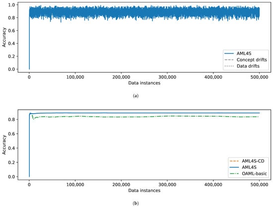
Figure 16.
Evaluation results of AML4S versus OAML-basic on the Hyperplane dataset, including (a) Accuracy of AML4S and different drifts of the Hyperplane dataset. (b) Moving average accuracy of AML4S versus OAML-basic on the Hyperplane dataset.
The effectiveness of our approach is also clear in Figure 16b, which depicts the accuracy of AML4S versus the OAML-basic algorithm for the Hyperplane data stream. Of course, the two configurations of AML4S achieve identical accuracy since, as already mentioned, no drifts of any type were detected in the data stream. In any case, both implementations outperform OAML-basic, indicating that AML4S can effectively adapt to online learning scenarios, even when no drifts are present.
Overall, it seems that AML4S is consistently more effective than the OAML-basic method in the different scenarios presented in this subsection. Table 9 summarizes our findings, presenting the accuracy values for OAML-basic and for the two configurations of AML4S, i.e., one with only concept drift detection (AML4S-CD) and one with both concept and data drift detection (AML4S). The largest difference in accuracy is observed for the Electricity dataset, which includes abrupt drifts. However, AML4S also outperforms OAML-basic on other cases, such as the Hyperplane dataset, which includes gradual drifts, or even the Airlines dataset, which includes a large number of drifts. Thus, we may conclude that AML4S is effective on multiple kinds of scenarios.
Table 9.
Accuracy of AML4S versus OAML-basic on four datasets (highest values highlighted using bold typeface).
Finally, concerning the comparison between AML4S-CD and the full version of OAML, it seems that the latter may achieve higher accuracy depending on the specifics of the dataset. For data streams with multiple features that may include both data and concept drifts, using a drift detection mechanism that detects both types of drifts is optimal. On the other hand, when the incoming data are not expected to contain any data drifts (i.e., when the features of the data stream are not prone to distribution changes), deactivating the data drift detection part of AML4S leads to identical results.
As in the previous experiment, Table 10 further depicts the average time required for our online methodology to process an instance (Mean Processing Time) and the average time required to train all pipelines (Mean Retraining Time). Concerning the Electricity, Airlines, and Hyperplane datasets, it is clear that the mean processing time is very short (less than one hundredth of a second), while the time required for full pipeline rebuilding is slightly more than 10 s. Therefore, we may consider AML4S as practical for real-time settings using these datasets. As for the Vehicle dataset, due to its large number of features (100), it exhibits higher processing times. However, in this case, it is also possible to maintain a (near-)real-time run as long as the instances arrive, e.g., in 2-minute or 3-minute intervals.
Table 10.
Mean processing and retraining times of AML4S on four datasets.
Finally, as in the previous evaluation experiment, once again, we perform the Wilcoxon signed rank test [32] to ensure that the higher accuracy of AML4S is statistically significant. Specifically, the mean accuracy of OAML is 0.78 (median 0.82), while the mean accuracy of AML4S is 0.83 (median 0.87). We use the one-tailed test, while the null hypothesis is that the two algorithms have equal (non-differing greatly) accuracy values (or even that OAML has higher accuracy). In this case, the Wilcoxon z statistic value is ; thus, the null hypothesis is rejected with a p-value of , meaning that the accuracy values of AML4S are significantly higher than those of OAML at .
5. Discussion and Threats to Validity
We acknowledge certain threats to validity and limitations of our approach and our evaluation. Those threats include the choice of the evaluation dataset and metrics, the choice of tools and algorithms/models used, as well as their limitations with respect to noise (and sensitivity to drifts) and class imbalance, and the limited comparison with other approaches.
Concerning the evaluation datasets, we may note that evaluating our approach was challenging, since current datasets and data generators focus mainly on concept drifts. Therefore, we created our own generator to evaluate our method in a more thorough setting. Since our generator includes drifts placed by hand, concerns about our method’s accuracy on a broader spectrum of problems may arise. To mitigate these concerns, we also evaluated our pipeline on a number of widely used datasets for drift detection (both real and synthetic) [30,31,33,34,35,36], illustrating how it ultimately yields better results, which is a testament to its generalization capabilities and its robustness. As for the (aggregated) accuracy, as our evaluation metric of choice, we opted for the most commonly used method in earlier work in the field [12,13,16,17]. However, we acknowledge that it may be a limitation of our method, and we plan to devise a more well-rounded evaluation framework in future work.
Regarding our choice of algorithms, we opted for a variety of methods, limited mainly by the options offered by the River framework [26]. For instance, River did not support online implementations for models such as SVMs or Neural Networks; therefore, we did not include them in our pipeline. However, we included an extensive (but not exhaustive) list of preprocessors (standard/min–max scaler), feature selectors (variance-based, similarity-based) and models (i.e., statistical, probabilistic, forests, instance-based), along with variety of hyperparameter ranges, to make our method more versatile and ensure enhanced performance across problems of different natures. In future work, we plan to explore the possibility of offering more choices, especially regarding preprocessing and parameter search space. Moreover, we plan on experimenting with different frameworks for online learning, such as MOA [37] or CapyMOA [38]. These frameworks also support sampling strategies, which could be used to address issues stemming from class imbalance as well as deep learning models, which can further enhance the performance and applicability of our system. Finally, potential inclusion of such models also prompts us to investigate the optimal memory size, or even employ automated methods for its tuning, in our future work.
Furthermore, the choice of drift detector may have a significant impact on the performance of our pipeline. ADWIN was selected for its robustness and versatility, meaning that it can handle various types of drifts, short-term noise, and evolving data distributions. However, it can also perform poorly in the presence of extreme noise patterns as well as multiple individual outliers. On the one hand, gradual drifts over a large time span may be detected too late or even remain undetected due to the statistical nature of the drift detector. These changes have to be handled by the online model itself, which should be able to effectively adjust to gradual/incremental distribution changes. On the other hand, sharp, random fluctuations may result in inaccurate drift detection, since these types of ‘spikes’/outliers in the data may be falsely regarded as drifts. As mentioned in Section 3.3, such phenomena are partially mitigated by the implementation of the buffer memory. However, in future work, we aim to address these issues by exploring alternative mitigation techniques, such as dynamically adjusting our detector’s sensitivity based on recent drift patterns, assessing the effectiveness of other noise-resilient drift detectors (e.g., EDDM [25]), or even combining drift detectors.
Finally, our comparison with other approaches on automated online machine learning was limited by the fact that such systems are currently few, while their implementations are often not available online. Nevertheless, we chose to at least compare our method with the OAML framework [16], for which we were able to find the results (the source code of the tool itself is not available at the time of writing). Although the OAML framework offers a number of methods for AutoML, we compare our approach to the OAML-basic method, since this is the method that our system most closely resembles. Thus, to ensure fair comparison, other variants, such as the OAML-ensemble or the OAML-model store, were not considered, as they rely on different prerequisites (e.g., OAML-ensemble builds ensembles of pipelines, while OAML-model store keeps a memory of models). However, as future work, we plan to investigate the possibility of enhancing AML4S using ensembles in order to further improve upon these variants. Finally, to aid researchers working in this direction, all data (the developed data generator) and scripts required to reproduce our findings are available online at https://github.com/AuthEceSoftEng/automl-data-streams (accessed on 22 August 2025).
6. Conclusions
As data today are produced in continuous flows of large volume and velocity, effective data stream mining has grown to be an important challenge. In this context, several research efforts have been directed towards effectively classifying instances of data streams and especially modeling shifts in the distributions of the data, known as drifts. However, contemporary approaches also have significant limitations; several of them are not automated, and may require manual parameter tuning. Even AutoML solutions typically focus only on concept drifts and do not always offer a complete pipeline that can adapt to different features and data drifts.
In this work, we created an online AutoML method that can be used on evolving data streams and can handle both data and concept drifts. Our method, AML4S, builds multiple pipelines automatically, including preprocessors, feature selectors, and classifiers, and assesses them in order to choose the best-performing one at each time, thus effectively adapting to distribution changes. It handles gradual changes using online models, while abrupt changes are handled by a drift detection mechanism. Upon evaluating AML4S, we found that it outperforms other online machine learning techniques, while it is also more effective than the state-of-the-art OAML-basic algorithm.
Our method is also not free of limitations, which are mainly centered around the choice of techniques, as well as the assessment of our pipeline. We denote as a limitation the choice of algorithms for our pipeline, bounded by the implementations of the River framework [26]. Including more algorithms and more configurations, along with a more extensive search space and advanced methods of hyperparameter tuning, would be an interesting extension to our pipeline. Moreover, our drift detector of choice, ADWIN, though robust and versatile in several cases, may be sensitive to scenarios with significant noise and/or extreme outliers (e.g., detecting multiple drifts that are false positives). Finally, from an assessment perspective, it is important to evaluate the aforementioned techniques in different scenarios. In this context, we have crafted our own data generator to specifically assess the performance of our method on data drift detection scenarios, while we have also included several other datasets in our evaluation, both synthetic and real, to evaluate its effectiveness. To further improve on this aspect and address the aforementioned limitations, it would be interesting to also include scenarios with extreme noise or multiple types of drifts so that we gain insights for refining our method.
In future work, we plan to further improve our method by taking action in several directions. First of all, it would be interesting to improve our drift detection mechanism by implementing techniques to mitigate occurrences of false positives or delayed drift detection, which are often observed at distributions with very frequent and/or gradual shifts. For instance, the parameters of ADWIN could be automatically adjusted according to the variance (distribution) of the dataset (e.g., the significance threshold discussed in Section 3.3 can be used to control the sensitivity of the algorithm to perceived drifts). Another idea would be to construct sliding windows of multiple feature values, effectively performing multivariate data drift detection. Moreover, we plan to further improve our AutoML pipeline selector by introducing an optimization strategy for selecting hyperparameters and finding the best pipeline. For that, Bayesian optimization [39] or Tree Parzen Estimators [40] seem to be promising options, since they offer effective and efficient pipeline-building. The former focuses on efficiently navigating the algorithm search space (preventing resource allocation to suboptimal configurations), while the latter allows for simultaneous evaluation of multiple configurations. Furthermore, we aim to expand our search space by including more preprocessing techniques and/or classification algorithms. It would be interesting to further explore the effectiveness of ensemble/deep learning methods [41,42,43] or even methods that could handle recurrent drifts by storing previous models to memory. And, in this aspect, it would also be beneficial to research the necessary optimizations to the buffer memory size and resource handling. Finally, we could further investigate the challenge of class imbalance in online learning [44] and investigate the combination of concept drift detectors with class imbalance handling techniques [45] in streaming data.
Author Contributions
Conceptualization, E.K., T.D., A.M. and A.L.S.; methodology, E.K., T.D., A.M. and A.L.S.; software, E.K., T.D., A.M. and A.L.S.; validation, E.K., T.D., A.M. and A.L.S.; formal analysis, E.K., T.D., A.M. and A.L.S.; investigation, E.K., T.D., A.M. and A.L.S.; resources, E.K., T.D., A.M. and A.L.S.; data curation, E.K., T.D., A.M. and A.L.S.; writing—original draft preparation, E.K., T.D., A.M. and A.L.S.; writing—review and editing, E.K., T.D., A.M. and A.L.S.; visualization, E.K., T.D., A.M. and A.L.S.; supervision, E.K., T.D., A.M. and A.L.S.; project administration, E.K., T.D., A.M. and A.L.S.; funding acquisition, E.K., T.D., A.M. and A.L.S. All authors have read and agreed to the published version of the manuscript.
Funding
This research received no external funding.
Data Availability Statement
The code and the data generator presented in this study are openly available on GitHub at https://github.com/AuthEceSoftEng/automl-data-streams (accessed on 22 August 2025).
Acknowledgments
Parts of this work were supported by the Horizon Europe project ECO-READY (Grant Agreement No. 101084201), funded by the European Union.
Conflicts of Interest
The authors declare no conflicts of interest.
Appendix A. Drift Functions of Loan Data Stream
In this appendix, we provide the different drift functions used by the Loan data generator that we crafted as part of our evaluation framework.
Appendix A.1. Data Drifts
For all scenarios, data drifts are simulated by the salary variable. Specifically, for the normal scenario, the salary in uniformly distributed in the range .
For the crisis scenario, the salary in uniformly distributed in the range .
For the growth scenario, the salary in uniformly distributed in the range .
Appendix A.2. Concept Drifts for Two Classes
For the scenario with two classes, the conditions are shown in Table A1.
Table A1.
Loan approval conditions for 2 classes.
Table A1.
Loan approval conditions for 2 classes.
| Normal | Crisis | Growth | |
|---|---|---|---|
| Approved | sv ← salary + 0.5 × commission | sv ← salary | sv ← salary + commission |
| loan ≤ 20 × sv | loan ≤ 10 × sv | loan ≤ 50 × sv | |
| loan ≤ 0.7 × housevalue | loan ≤ 0.5 × housevalue | loan ≤ 0.9 × housevalue | |
| age < 20 ∧ sv ≥ 20,000 | age < 20 ∧ sv ≥ 30,000 | age < 20 ∧ sv ≥ 10,000 | |
| age < 40 ∧ sv ≥ 25,000 | age < 40 ∧ sv ≥ 40,000 | age < 40 ∧ sv ≥ 15,000 | |
| age < 60 ∧ sv ≥ 30,000 | age < 60 ∧ sv ≥ 50,000 | age < 60 ∧ sv ≥ 20,000 | |
| Declined | All other cases | ||
Appendix A.3. Concept Drifts for Three Classes
For the scenario with three classes, the conditions are shown in Table A2.
Table A2.
Loan approval conditions for 3 classes.
Table A2.
Loan approval conditions for 3 classes.
| Normal | Crisis | Growth | |
|---|---|---|---|
| Approved | sv ← salary + 0.5 × commission | sv ← salary | sv ← salary + commission |
| loan ≤ 20 × sv | loan ≤ 10 × sv | loan ≤ 50 × sv | |
| loan ≤ 0.7 × housevalue | loan ≤ 0.5 × housevalue | loan ≤ 0.9 × housevalue | |
| age < 40 ∧ sv ≥ 25,000 | age < 40 ∧ sv ≥ 40,000 | age < 40 ∧ sv ≥ 15,000 | |
| age < 50 ∧ sv ≥ 30,000 | age < 50 ∧ sv ≥ 50,000 | age < 50 ∧ sv ≥ 20,000 | |
| age < 65 ∧ sv ≥ 45,000 | age < 65 ∧ sv ≥ 60,000 | age < 65 ∧ sv ≥ 35,000 | |
| Conditionally | sv ← salary + 0.5 × commission | sv ← salary | sv ← salary + commission |
| Approved | loan ≤ 20 × sv | loan ≤ 10 × sv | loan ≤ 50 × sv |
| loan ≤ 0.7 × housevalue | loan ≤ 0.5 × housevalue | loan ≤ 0.9 × housevalue | |
| age < 40 ∧ sv ≥ 17,000 | age < 40 ∧ sv ≥ 30,000 | age < 40 ∧ sv ≥ 10,000 | |
| age < 50 ∧ sv ≥ 25,000 | age < 50 ∧ sv ≥ 45,000 | age < 50 ∧ sv ≥ 15,000 | |
| age < 65 ∧ sv ≥ 30,000 | age < 65 ∧ sv ≥ 50,000 | age < 65 ∧ sv ≥ 20,000 | |
| Declined | All other cases | ||
Appendix A.4. Concept Drifts for Four Classes
For the scenario with four classes, the conditions are shown in Table A3.
Table A3.
Loan approval conditions for 4 classes.
Table A3.
Loan approval conditions for 4 classes.
| Normal | Crisis | Growth | |
|---|---|---|---|
| Approved | sv ← salary + 0.5 × commission | sv ← salary | sv ← salary + commission |
| loan ≤ 20 × sv | loan ≤ 10 × sv | loan ≤ 50 × sv | |
| loan ≤ 0.7 × housevalue | loan ≤ 0.5 × housevalue | loan ≤ 0.9 × housevalue | |
| age < 40 ∧ sv ≥ 26,000 | age < 40 ∧ sv ≥ 41,000 | age < 40 ∧ sv ≥ 16,000 | |
| age < 50 ∧ sv ≥ 31,000 | age < 50 ∧ sv ≥ 50,000 | age < 50 ∧ sv ≥ 20,000 | |
| age < 65 ∧ sv ≥ 45,000 | age < 65 ∧ sv ≥ 60,000 | age < 65 ∧ sv ≥ 35,000 | |
| Conditionally | sv ← salary + 0.5 × commission | sv ← salary | sv ← salary + commission |
| Approved | loan ≤ 20 × sv | loan ≤ 10 × sv | loan ≤ 50 × sv |
| loan ≤ 0.7 × housevalue | loan ≤ 0.5 × housevalue | loan ≤ 0.9 × housevalue | |
| age < 40 ∧ sv ≥ 23,000 | age < 40 ∧ sv ≥ 36,000 | age < 40 ∧ sv ≥ 13,000 | |
| age < 50 ∧ sv ≥ 27,000 | age < 50 ∧ sv ≥ 44,000 | age < 50 ∧ sv ≥ 16,000 | |
| age < 65 ∧ sv ≥ 40,000 | age < 65 ∧ sv ≥ 53,000 | age < 65 ∧ sv ≥ 29,000 | |
| Exceptionally | sv ← salary + 0.5 × commission | sv ← salary | sv ← salary + commission |
| Declined | loan ≤ 20 × sv | loan ≤ 20 × sv | loan ≤ 20 × sv |
| loan ≤ 0.7 × housevalue | loan ≤ 0.7 × housevalue | loan ≤ 0.7 × housevalue | |
| age < 40 ∧ sv ≥ 19,000 | age < 40 ∧ sv ≥ 32,000 | age < 40 ∧ sv ≥ 10,000 | |
| age < 50 ∧ sv ≥ 23,000 | age < 50 ∧ sv ≥ 38,000 | age < 50 ∧ sv ≥ 14,000 | |
| age < 65 ∧ sv ≥ 35,000 | age < 65 ∧ sv ≥ 45,000 | age < 65 ∧ sv ≥ 23,000 | |
| Declined | All other cases | ||
References
- Sagiroglu, S.; Sinanc, D. Big data: A review. In Proceedings of the 2013 International Conference on Collaboration Technologies and Systems (CTS), San Diego, CA, USA, 20–24 May 2013; pp. 42–47. [Google Scholar] [CrossRef]
- Agrahari, S.; Singh, A.K. Concept Drift Detection in Data Stream Mining: A literature review. J. King Saud Univ.—Comput. Inf. Sci. 2022, 34, 9523–9540. [Google Scholar] [CrossRef]
- Gama, J.A.; Žliobaitė, I.; Bifet, A.; Pechenizkiy, M.; Bouchachia, A. A survey on concept drift adaptation. ACM Comput. Surv. 2014, 46, 1–37. [Google Scholar] [CrossRef]
- Lu, J.; Liu, A.; Dong, F.; Gu, F.; Gama, J.; Zhang, G. Learning under Concept Drift: A Review. IEEE Trans. Knowl. Data Eng. 2019, 31, 2346–2363. [Google Scholar] [CrossRef]
- Gomes, H.M.; Read, J.; Bifet, A.; Barddal, J.P.; Gama, J. Machine learning for streaming data: State of the art, challenges, and opportunities. SIGKDD Explor. Newsl. 2019, 21, 6–22. [Google Scholar] [CrossRef]
- Bifet, A.; Gavaldà, R. Adaptive Learning from Evolving Data Streams. In Advances in Intelligent Data Analysis VIII: 8th International Symposium on Intelligent Data Analysis, IDA 2009, Lyon, France, 31 August–2 September 2009; Springer: Berlin/Heidelberg, Germany, 2009; pp. 249–260. [Google Scholar] [CrossRef]
- Bifet, A.; Holmes, G.; Pfahringer, B. Leveraging bagging for evolving data streams. In Machine Learning and Knowledge Discovery in Databases: European Conference, ECML PKDD 2010, Barcelona, Spain, 20–24 September 2010. Proceedings, Part I; Springer: Berlin/Heidelberg, Germany, 2010; pp. 135–150. [Google Scholar]
- Gomes, H.M.; Bifet, A.; Read, J.; Barddal, J.P.; Enembreck, F.; Pfharinger, B.; Holmes, G.; Abdessalem, T. Adaptive random forests for evolving data stream classification. Mach. Learn. 2017, 106, 1469–1495. [Google Scholar] [CrossRef]
- Gomes, H.M.; Read, J.; Bifet, A. Streaming Random Patches for Evolving Data Stream Classification. In Proceedings of the 2019 IEEE International Conference on Data Mining (ICDM), Beijing, China, 8–11 November 2019; pp. 240–249. [Google Scholar] [CrossRef]
- Rad, R.H.; Haeri, M.A. Hybrid Forest: A Concept Drift Aware Data Stream Mining Algorithm. arXiv 2019, arXiv:1902.03609. [Google Scholar] [CrossRef]
- Yang, L.; Manias, D.M.; Shami, A. PWPAE: An Ensemble Framework for Concept Drift Adaptation in IoT Data Streams. In Proceedings of the 2021 IEEE Global Communications Conference (GLOBECOM), Madrid, Spain, 7–11 December 2021; pp. 1–6. [Google Scholar] [CrossRef]
- Madrid, J.G.; Jair Escalante, H.; Morales, E.F.; Tu, W.W.; Yu, Y.; Sun-Hosoya, L.; Guyon, I.; Sebag, M. Towards AutoML in the presence of Drift: First results. In Proceedings of the Workshop AutoML 2018 @ ICML/IJCAI-ECAI, Stockholm, Sweden, 14 July 2018. [Google Scholar]
- Kulbach, C.; Montiel, J.; Bahri, M.; Heyden, M.; Bifet, A. Evolution-Based Online Automated Machine Learning. In Advances in Knowledge Discovery and Data Mining: 26th Pacific-Asia Conference, PAKDD 2022, Chengdu, China, 16–19 May 2022, Proceedings, Part I; Springer: Cham, Switzerland, 2022; pp. 472–484. [Google Scholar] [CrossRef]
- Bahri, M.; Georgantas, N. AutoClass: AutoML for Data Stream Classification. In Proceedings of the 2023 IEEE International Conference on Big Data (BigData), Sorrento, Italy, 15–18 December 2023; pp. 2658–2666. [Google Scholar] [CrossRef]
- Wu, Q.; Wang, C.; Langford, J.; Mineiro, P.; Rossi, M. ChaCha for Online AutoML. In Proceedings of the 38th International Conference on Machine Learning. Proc. Mach. Learn. Res. 2021, 139, 11263–11273. [Google Scholar]
- Celik, B.; Singh, P.; Vanschoren, J. Online AutoML: An adaptive AutoML framework for online learning. Mach. Learn. 2022, 112, 1897–1921. [Google Scholar] [CrossRef]
- Verma, N.; Bifet, A.; Pfahringer, B.; Bahri, M. ASML: A Scalable and Efficient AutoML Solution for Data Streams. In Proceedings of the AutoML 2024—International Conference on Automated Machine Learning, Paris, France, 9–12 December 2024. [Google Scholar]
- Nguyen, H.L.; Woon, Y.K.; Ng, W.K. A survey on data stream clustering and classification. Knowl. Inf. Syst. 2015, 45, 535–569. [Google Scholar] [CrossRef]
- Gözüaçık, O.; Can, F. Concept learning using one-class classifiers for implicit drift detection in evolving data streams. Artif. Intell. Rev. 2021, 54, 3725–3747. [Google Scholar] [CrossRef]
- Bifet, A.; Gavalda, R. Learning from Time-Changing Data with Adaptive Windowing. In Proceedings of the 2007 SIAM International Conference on Data Mining (SDM), Minneapolis, MI, USA, 26–28 April 2007; pp. 443–448. [Google Scholar] [CrossRef]
- Oza, N.C.; Russell, S.J. Online Bagging and Boosting. In Proceedings of the Eighth International Workshop on Artificial Intelligence and Statistics, Key West, FL, USA, 4–7 January 2001; pp. 229–236. [Google Scholar]
- Feurer, M.; Klein, A.; Eggensperger, K.; Springenberg, J.T.; Blum, M.; Hutter, F. Efficient and robust automated machine learning. In Proceedings of the 29th International Conference on Neural Information Processing Systems (NIPS’15), Montreal, QC, Canada, 7–12 December 2015; Volume 2, pp. 2962–2970. [Google Scholar]
- Pesaranghader, A.; Viktor, H.L. Fast Hoeffding Drift Detection Method for Evolving Data Streams. In Proceedings of the Machine Learning and Knowledge Discovery in Databases, Riva del Garda, Italy, 19–23 September 2016; pp. 96–111. [Google Scholar]
- Bäck, T. Evolutionary Algorithms in Theory and Practice: Evolution Strategies, Evolutionary Programming, Genetic Algorithms; Oxford University Press: Oxford, UK, 1996. [Google Scholar] [CrossRef]
- Baena-Garcıa, M.; del Campo-Ávila, J.; Fidalgo, R.; Bifet, A. Early drift detection method. In Proceedings of the Fourth International Workshop on Knowledge Discovery from Data Streams, Philadelphia, PA, USA, 20 August 2006; Volume 6, pp. 77–86. [Google Scholar]
- Montiel, J.; Halford, M.; Mastelini, S.M.; Bolmier, G.; Sourty, R.; Vaysse, R.; Zouitine, A.; Gomes, H.M.; Read, J.; Abdessalem, T.; et al. River: Machine learning for streaming data in Python. J. Mach. Learn. Res. 2021, 22, 1–8. [Google Scholar]
- González, M.L.; Sedano, J.; García-Vico, Á.M.; Villar, J.R. A Comparison of Techniques for Virtual Concept Drift Detection. In 16th International Conference on Soft Computing Models in Industrial and Environmental Applications (SOCO 2021); Springer: Cham, Switzerland, 2022; pp. 3–13. [Google Scholar]
- Mahgoub, M.; Moharram, H.; Elkafrawy, P.; Awad, A. Benchmarking Concept Drift Detectors for Online Machine Learning. In Model and Data Engineering: 11th International Conference, MEDI 2022, Cairo, Egypt, 21–24 November 2022; Springer: Cham, Switzerland, 2023; pp. 43–57. [Google Scholar] [CrossRef]
- Agrawal, R.; Imielinski, T.; Swami, A. Database Mining: A Performance Perspective. IEEE Trans. Knowl. Data Eng. 1993, 5, 914–925. [Google Scholar] [CrossRef]
- Blackard, J. Covertype. In UCI Machine Learning Repository; University of California: Irvine, CA, USA, 1998. [Google Scholar] [CrossRef]
- Losing, V.; Hammer, B.; Wersing, H. KNN Classifier with Self Adjusting Memory for Heterogeneous Concept Drift. In Proceedings of the 2016 IEEE 16th International Conference on Data Mining (ICDM), Barcelona, Spain, 12–15 December 2016; pp. 291–300. [Google Scholar] [CrossRef]
- Wilcoxon, F. Individual Comparisons by Ranking Methods. Biom. Bull. 1945, 1, 80–83. [Google Scholar] [CrossRef]
- Harries, M. Splice-2 Comparative Evaluation: Electricity Pricing; Technical Report UNSW-CSE-TR-9905; University of New South Wales, School of Computer Science and Engineering: Sydney, NSW, Australia, 1999. [Google Scholar]
- Duarte, M.F.; Hu, Y.H. Vehicle classification in distributed sensor networks. J. Parallel Distrib. Comput. 2004, 64, 826–838. [Google Scholar] [CrossRef]
- Bifet, A.; Holmes, G.; Pfahringer, B.; Read, J.; Kranen, P.; Kremer, H.; Jansen, T.; Seidl, T. MOA: A real-time analytics open source framework. In Machine Learning and Knowledge Discovery in Databases, Part III: European Conference, ECML PKDD 2010, Athens, Greece, 5–9 September 2011, Proceedings, Part III; Springer: Berlin/Heidelberg, Germany, 2011; pp. 617–620. [Google Scholar]
- Hulten, G.; Spencer, L.; Domingos, P. Mining time-changing data streams. In Proceedings of the Seventh ACM SIGKDD International Conference on Knowledge Discovery and Data Mining, KDD ’01, New York, NY, USA, 26–29 August 2001; pp. 97–106. [Google Scholar] [CrossRef]
- Bifet, A.; Holmes, G.; Kirkby, R.; Pfahringer, B. MOA: Massive Online Analysis, a Framework for Stream Classification and Clustering. J. Mach. Learn. Res. 2010, 11, 1601–1604. [Google Scholar]
- Gomes, H.M.; Bifet, A. Practical Machine Learning for Streaming Data. In Proceedings of the 30th ACM SIGKDD Conference on Knowledge Discovery and Data Mining, KDD ’24, New York, NY, USA, 25–29 August 2024; pp. 6418–6419. [Google Scholar] [CrossRef]
- Snoek, J.; Larochelle, H.; Adams, R.P. Practical Bayesian optimization of machine learning algorithms. In Proceedings of the 25th International Conference on Neural Information Processing Systems (NIPS’12), Granada, Spain, 12–15 December 2011; Volume 2, pp. 2951–2959. [Google Scholar]
- Bergstra, J.; Bardenet, R.; Bengio, Y.; Kégl, B. Algorithms for hyper-parameter optimization. In Proceedings of the 24th International Conference on Neural Information Processing Systems (NIPS’11), Vancouver, BC, Canada, 6–9 December 2010; pp. 2546–2554. [Google Scholar]
- Hu, L.; Lu, Y.; Feng, Y. Concept Drift Detection Based on Deep Neural Networks and Autoencoders. Appl. Sci. 2025, 15, 3056. [Google Scholar] [CrossRef]
- Wang, P.; Jin, N.; Davies, D.; Woo, W.L. Model-centric transfer learning framework for concept drift detection. Knowl.-Based Syst. 2023, 275, 110705. [Google Scholar] [CrossRef]
- Yu, H.; Zhang, Q.; Liu, T.; Lu, J.; Wen, Y.; Zhang, G. Meta-ADD: A meta-learning based pre-trained model for concept drift active detection. Inf. Sci. 2022, 608, 996–1009. [Google Scholar] [CrossRef]
- Wang, S.; Minku, L.L.; Yao, X. A Systematic Study of Online Class Imbalance Learning with Concept Drift. IEEE Trans. Neural Netw. Learn. Syst. 2018, 29, 4802–4821. [Google Scholar] [CrossRef]
- Priya, S.; Uthra, R.A. Deep learning framework for handling concept drift and class imbalanced complex decision-making on streaming data. Complex Intell. Syst. 2023, 9, 3499–3515. [Google Scholar] [CrossRef]
Disclaimer/Publisher’s Note: The statements, opinions and data contained in all publications are solely those of the individual author(s) and contributor(s) and not of MDPI and/or the editor(s). MDPI and/or the editor(s) disclaim responsibility for any injury to people or property resulting from any ideas, methods, instructions or products referred to in the content. |
© 2025 by the authors. Licensee MDPI, Basel, Switzerland. This article is an open access article distributed under the terms and conditions of the Creative Commons Attribution (CC BY) license (https://creativecommons.org/licenses/by/4.0/).