Article

An Efficient and Accurate Random Forest Node-Splitting Algorithm Based on Dynamic Bayesian Methods

1
School of Physics, Central South University, Changsha 410083, China
2
School of Electronic Information, Central South University, Changsha 410075, China
*
Author to whom correspondence should be addressed.
Mach. Learn. Knowl. Extr. 2025, 7(3), 70; https://doi.org/10.3390/make7030070
Submission received: 6 June 2025 / Revised: 12 July 2025 / Accepted: 17 July 2025 / Published: 21 July 2025

Abstract

Random Forests are powerful machine learning models widely applied in classification and regression tasks due to their robust predictive performance. Nevertheless, traditional Random Forests face computational challenges during tree construction, particularly in high-dimensional data or on resource-constrained devices. In this paper, a novel node-splitting algorithm, BayesSplit, is proposed to accelerate decision tree construction via a Bayesian-based impurity estimation framework. BayesSplit treats impurity reduction as a Bernoulli event with Beta-conjugate priors for each split point and incorporates two main strategies. First, Dynamic Posterior Parameter Refinement updates the Beta parameters based on observed impurity reductions in batch iterations. Second, Posterior-Derived Confidence Bounding establishes statistical confidence intervals, efficiently filtering out suboptimal splits. Theoretical analysis demonstrates that BayesSplit converges to optimal splits with high probability, while experimental results show up to a 95% reduction in training time compared to baselines and maintains or exceeds generalization performance. Compared to the state-of-the-art MABSplit, BayesSplit achieves similar accuracy on classification tasks and reduces regression training time by 20–70% with lower MSEs. Furthermore, BayesSplit enhances feature importance stability by up to 40%, making it particularly suitable for deployment in computationally constrained environments.

1. Introduction

It is widely known that the performance of multiple combined classifiers far exceeds that of using any single classifier independently [1]. Tree ensembles such as Random Forest (RF) [2] have achieved impressive success across various classification and regression tasks. RF builds a number of decision trees in the training process, which contributes to the final outcome through an aggregation method known as bagging [3]. Each decision tree is built using a bootstrap sample of the data and random subsets of features at each split. The predictions from decision trees are combined to produce the final output of RF, delivering high accuracy and robustness across different datasets and outperforming single classifiers, especially on complex predictive tasks [4].
RF has established itself as an indispensable tool in data mining, with applications covering bioinformatics [5], image processing [6], financial analytics [7], and natural language processing [8]. However, traditional RF algorithms face substantial challenges when handling high-dimensional data or running on hardware-constrained devices such as smartphones and Internet-of-Things (IoT) systems [9]. In these scenarios, the traditional algorithms often exhibit lower computational efficiency and reduced predictive accuracy. These limitations become even more pronounced due to the rapidly evolving computational landscape, where edge computing and IoT devices demand faster and more reliable algorithms [10].
To address these computational demands, researchers have explored various optimization techniques, particularly those focusing on decision-tree construction [11]. Decision trees represent the relationship between features and target variables through a hierarchical structure of conjunctive conditions, where each internal node corresponds to a feature and a threshold. In RF, finding the optimal split by identifying the best feature–threshold pair is crucial for both computational efficiency and predictive accuracy [12]. Accordingly, optimizing the node splitting process can significantly improve the overall performance of RF [13].
The traditional RF algorithms determine optimal splits by exhaustively searching through all possible splitting points, resulting in a computational complexity of  O N  for each split, where   N   is the number of instances. They are computationally heavy and inefficient. To address this problem, algorithms like XGBoost [14] and LightGBM [15] have employed histogram-based techniques to reduce the complexity to  O B , where  B N , by grouping feature values into discrete bins. While histogram-based methods can substantially accelerate training, they remain wasteful because they allocate the same computational effort to all features, including those that are not particularly informative.

1.1. Related Works

In 2001, Breiman [2] introduced the RF algorithm by combining the bagging technique, the random subspace method, and the Classification and Regression Trees (CART) algorithm. With the rapid growth of information technology, datasets have expanded dramatically in both size and complexity. Traditional RF algorithms face significant challenges meeting time and computational demands [16]. Thus, enhancing RFs to handle large datasets has become a major focus in both research and industry [17].
Recent advancements have emerged in algorithmic optimizations and parallel computing techniques. Yates and Islam [9] developed FastForest, which incorporates Subbagging to reduce the size of bootstrap samples, Logarithmic Split-Point Sampling (LSPS) to decrease the computational cost of node splits, and Dynamic Restricted Subspacing (DRS) to adjust the feature subset size during feature selection. These optimizations collectively reduce the data processed by each tree, thereby accelerating node splitting. In the context of incremental learning, Domingos and Hulten [18] introduced Hoeffding Tree (HT) in Very Fast Decision Tree (VFDT), which utilizes the Hoeffding Bound to guide the choice of decision nodes, ensuring a rapid and effective approximation of the optimal decision with limited samples. The Extremely Fast Decision Tree (EFDT) algorithm [19] builds upon HT by introducing Hoeffding Anytime Tree (HATT), which continuously monitors and updates splits as more data becomes available. Both HT and HATT are incremental decision tree learning techniques, particularly suited for big data environments and data stream applications.
Parallel computing frameworks have also been leveraged to enhance decision tree algorithms. Mu et al. [20] proposed a parallel decision tree algorithm based on MapReduce, using Pearson’s correlation coefficient for optimal split selection. Xu [21] introduced an improved RF algorithm based on Spark, leveraging the Fayyad boundary point principle for efficient feature discretization. Yin et al. [22] presented a fast parallel RF algorithm on Spark, integrating a modified Gini coefficient to reduce feature redundancy and applying an approximate equal-frequency binning method for split optimization.
Although these algorithms have sped up the training process for decision tree ensembles, most of them still rely on exhaustive searches to find the optimal split at each node, which can be costly for large datasets. MABSplit presents a cutting-edge solution to overcome this bottleneck [23]. At its core, MABSplit treats each candidate feature–threshold pair as an arm in a multi-armed bandit (MAB) problem, aiming to efficiently identify the optimal split by estimating each candidate’s impurity reduction through sampling. Specifically, the algorithm iteratively samples batches of data points, updates confidence intervals of impurity reduction estimates for each candidate split, and eliminates splits whose lower confidence bound exceeds the upper confidence bound of the currently best-performing candidate. This adaptive procedure significantly reduces computational complexity from linear to logarithmic with respect to the number of samples, achieving substantial speed-ups without compromising predictive accuracy.
Despite its considerable strengths, MABSplit has certain aspects that could be further enhanced:
Lack of Memory Mechanism: MABSplit lacks some related mechanisms to leverage information gathered from previously explored splits. The valuable information from earlier computations is not utilized to improve subsequent split evaluations. Consequently, the exploration in the early phase would be less efficient.
Lower Efficiency for Similar Candidates: The computational efficiency of MABSplit relies on sufficient heterogeneity among the true impurity reductions of different feature–threshold pairs. When most splits have similar impurity reductions (as in highly symmetric datasets), MABSplit fails to achieve its promised logarithmic sample complexity and reduces to a batched version of the naïve approach, resulting in no significant speed advantage.
Reduced Accuracy with Limited Samples: MABSplit employs confidence intervals to estimate split quality, which are derived from some statistical properties of impurity measures such as Gini impurity and entropy. However, these estimates may become less reliable when sample sizes are small or probabilities approach extreme values.

1.2. Our Contributions

In this paper, we introduce BayesSplit, a novel node-splitting algorithm that extends MABSplit to improve the computational efficiency and predictive accuracy of RFs. BayesSplit treats the probability of impurity reduction as a Beta posterior distribution, which is iteratively refined based on batched observations. Based on this, posterior confidence intervals are used to adaptively select splits most likely to maximize impurity reduction, ensuring statistically robust and data-driven tree construction. Our key contributions include:
(1) A Novel Bayesian-Based Impurity Estimation Framework
A Bayesian framework is developed that treats each split’s impurity reduction as a random event with an unknown success probability. The framework initializes uninformative Beta priors that evolve into informative posteriors as observations accumulate. After each batch of samples is evaluated, the Beta parameters of candidate splits are updated according to the observed impurity reductions. These posterior distributions are used to derive confidence intervals that balance exploration of uncertain splits with exploitation of promising ones. By comparing the confidence bounds of each split across all candidates, BayesSplit eliminates suboptimal splits while allocating computational resources to the most promising candidates. This Bayesian-based Impurity Estimation Framework naturally accommodates prior knowledge and new data, enabling robust decision-making and faster convergence to optimal splits.
(2) Two Bayesian Optimization Strategies to Achieve High Computational Efficiency
Dynamic Posterior Parameter Refinement: Drawing inspiration from Thompson Sampling (TS), this strategy treats each split’s impurity reduction as a reward signal to update the parameters of Beta distributions. After a batch is sampled, whether each split reduced impurity is evaluated,  α   is incremented when impurity decreases and  β   when it does not. This process creates a memory mechanism to accumulate evidence across iterations.
Posterior-Derived Confidence Bounding: This strategy uses each split’s posterior Beta distribution to establish confidence intervals. Rather than relying on frequentist approximations, the confidence bounds are set directly from the posterior parameters, enabling more accurate uncertainty quantification across diverse data conditions.
Our experiment results demonstrate that BayesSplit further minimizes quantization errors and more accurately captures the underlying data distribution than existing approaches.

2. Algorithmic Background

To facilitate understanding of the subsequent technical content, we summarize the key notation used in this paper. Table 1 provides a list of symbols and their meanings, serving as a reference for the algorithmic development and theoretical analysis of BayesSplit.

2.1. Node-Splitting Description in RFs and Decision Trees

An RF is composed of multiple classification or regression trees, where each tree   T   maps the feature space to the response. Consider a dataset   D   with   N   data points  x i , y i i = 1 N , where   x i   is the   i -th feature vector and  y i   is the corresponding target. Each tree in an RF is built independently on a bootstrapped dataset  D T   from the original data   D , while a random subset of features M   is considered at each node.
In the decision tree node-splitting process, let  R ν   represent the region in the feature space corresponding to node   ν  (typically a hyper-rectangle) [24]. Using the pair   f , t   to split node   ν R ν   is partitioned into two subregions   R ν , l e f t   and  R ν , r i g h t   , corresponding to the left and right child nodes of node   ν . For a node  ν  in decision tree  T N n ν = i D T : x i R ν   denotes the number of samples falling into  R ν . Finding the optimal split, i.e., determining the best pair  f b , t b   to maximize node-splitting effectiveness, is accomplished by maximizing the reduction in label impurity:
argmin f M , t T N n ν l e f t N n ν I ν l e f t + N n ν r i g h t N n ν I ν r i g h t I ν
where   N n ν l e f t   and   N n ν r i g h t   represent the number of samples in the left and right child nodes, respectively,  I ·   represents the impurity measure, and   T   denotes the permissible thresholds for feature  f . Popular impurity measures include the Gini index and entropy for classification, as well as the mean-squared error (MSE) for regression [25]:
G i n i = 1 k = 1 K p k 2
E = k = 1 K p k log 2 p k
M S E = 1 N n v i : x i R v y i y ¯ 2
where  K  represents the no. of classes in the target variable,  p k   is the proportion of samples at node belonging to class   k , and  y ¯   is calculated as  y ¯ = 1 N n v i : x i R v y i . In Equation (1),  I ν   denotes the impurity of node   ν  before splitting and does not depend on the split feature  f  or threshold  t . Since  I ν  does not affect the minimization process, we simplify Equations (1)–(5) for a direct evaluation of the split effect, written as follows:
argmin f M , t T N n ν l e f t N n ν I ν l e f t + N n ν r i g h t N n ν I ν r i g h t
We define  μ f t = N n ν l e f t N n ν I ν l e f t + N n ν r i g h t N n ν I ν r i g h t   as the optimization objective. Note that lower values of  μ f t   correspond to higher impurity reductions, while higher values of  μ f t   correspond to lower impurity reductions.

2.2. Confidence Interval Estimation in MABSplit

Since computing  μ f t   exactly requires a full pass over the data, MABSplit draws  n   samples,  X i , Y i i = 1 n , to construct point estimates  μ ^ f t   and confidence intervals for impurity reduction. At the core of this approach is the delta method, which transforms the empirical estimates of class distributions into reliable estimates of impurity measures.
Let   p L , k   and  p R , k   represent the proportion of the full data points in class   k   and each of the two subsets created by the split  f , t . For a given split  f , t ,  MABSplit constructs empirical estimates  p ^ L , k   and  p ^ R , k   represents the proportion of class   k   samples in the left and right child nodes based on the  n   subsamples, respectively:
p ^ L , k   = 1 n i = 1 n I X i f < t ,   Y i = k p ^ R , k   = 1 n i = 1 n I X i f t ,   Y i = k  
These estimates jointly follow a multinomial distribution with parameters  n , p , where  p = p L , 1 , , p L , K , p R , 1 , , p R , K T . By the Central Limit Theorem (CLT), we obtain the following:
n γ ^ γ d N 0 , Q γ  
where  γ = p L , 1 , , p L , K , p R , 1 , , p R , K 1 T  and  γ ^ = p ^ L , 1 , , p ^ L , K 1 , p ^ R , 1 , , p ^ R , K 1 T Q γ  is the corresponding covariance matrix. Specifically,  μ f t  could be written in terms of  γ  for the impurity metrics (e.g., Gini or entropy). Let  μ f t γ  be the derivative of  μ f t  with respect to  γ . Applying the delta method, we obtain the following:
n μ ^ f t γ μ f t γ d N 0 , μ f t γ T Q γ μ f t γ  
This allows MABSplit to construct  1 δ  confidence intervals scale as  C f t n , δ = O log 1 / δ / n , these confidence intervals are asymptotically valid as  n . In MABSplit, each batch of data points updates  p ^ L , k   and  p ^ R , k , which in turn refine the point estimates  μ ^ f t   and their corresponding confidence intervals.
While the delta method provides a theoretically sound framework for constructing confidence intervals, its practical reliability depends on the validity of asymptotic assumptions guaranteed by the CLT. Specifically, Equation (8) shows that the width of the confidence intervals depends on the sample size through a   1 / n   scaling. In the early stages of MABSplit, where only small batches of data are available, this approximation may break down. For example, when the class proportions approach 0, the derivative of impurity metrics such as entropy becomes unstable, leading to large variance and unreliable confidence intervals.
In summary, MABSplit exhibits reduced accuracy with limited samples, as statistical estimation under small-sample conditions can introduce substantial variance in impurity estimates.

3. BayesSplit: A Bayesian Node-Splitting Algorithm

3.1. Overview of the Framework

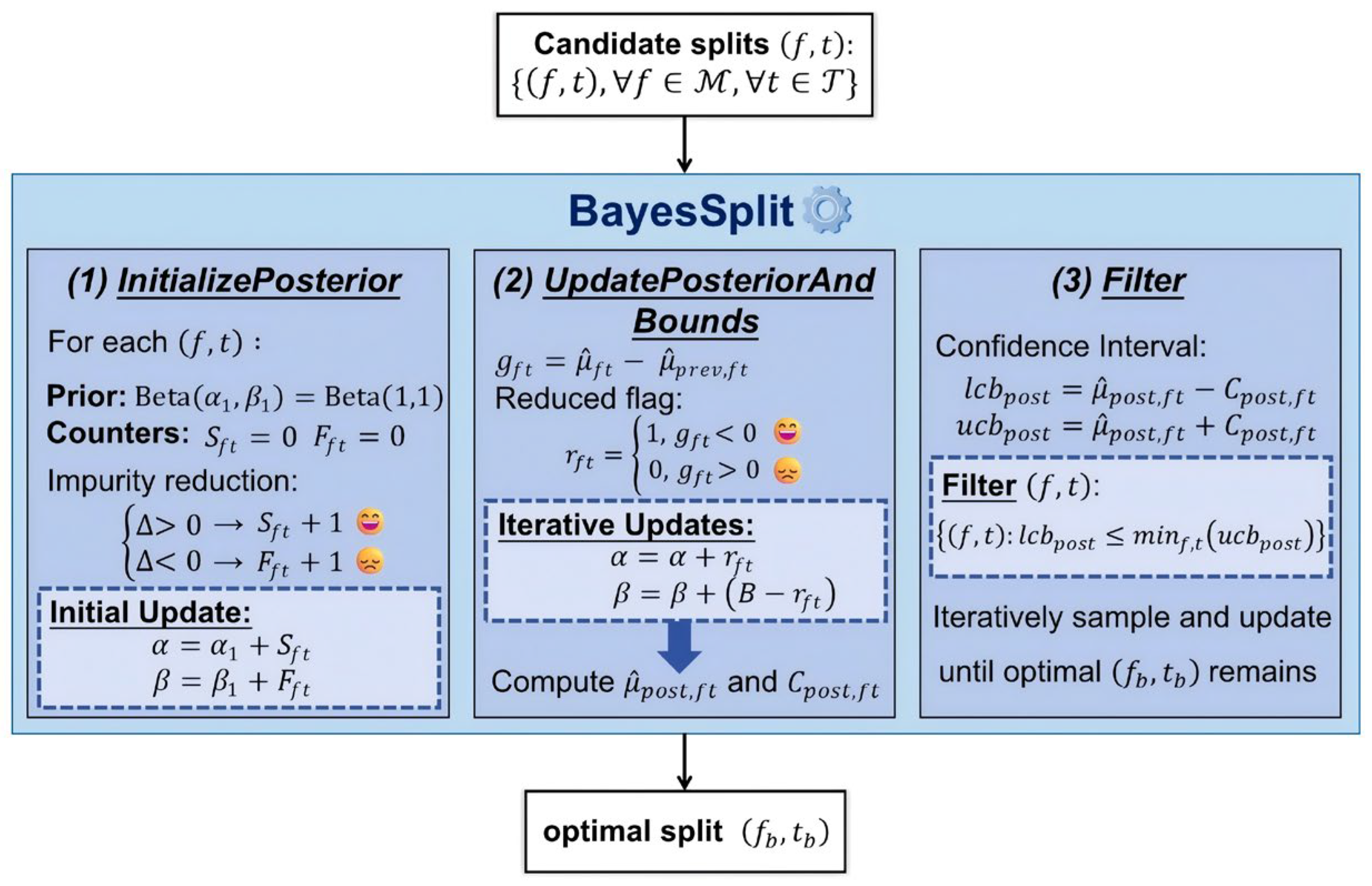
BayesSplit treats impurity reduction as a Bernoulli event with Beta-conjugate priors, as shown in Figure 1. The framework begins with uninformative priors, which are gradually updated into informative posteriors as observations accumulate. After each batch of samples is evaluated, the Beta parameters of candidate splits are updated based on the observed impurity reductions.
The framework consists of three key components: (1) InitializePosterior establishes posterior distributions for each candidate split based on initial impurity evaluations; (2) UpdatePosteriorAndBounds implements the Dynamic Posterior Parameter Refinement strategy, updating beliefs about split effectiveness based on empirical observations; and (3) Filter uses Posterior-Derived Confidence Bounds to eliminate splits that are demonstrably suboptimal, focusing resources on promising candidates.
The precise splitting approach BayesSplit is outlined in Algorithm 1. We preprocess the input data to identify candidate splits    f , t , or arms, for each feature   f . All potential solutions to Equation (5) are tracked by maintaining a set  S solution , which initially includes every candidate arm   f , t .
Algorithm 1 BayesSplit  ( X , M , T , I , B )
  1:
S solution { f , t , f M , t T }  // Set of potential solutions to Equation (5)
  2:
n u s e d 0  // Number of data points sampled
  3:
for all  ( f , t ) S s o l u t i o n  do
  4:
μ ^ f t , C f t  // Initialize mean and CI for each arm
  5:
end for
  6:
for all  f M  do
  7:
 Create empty histogram  h f  with  T = T  equally spaced bins
  8:
end for
  9:
InitializePosterior // Set up posterior distributions
10:
while  n u s e d < n   and   S s o l u t i o n > 1  do
11:
 Draw a batch sample  X b a t c h  of size B with replacement from  X
12:
for all unique f in Ssolution do
13:
  for all x in  X batch  do
14:
   Insert xf into histogram hf // Update histograms with sampled data
15:
  end for
16:
end for
17:
for all  ( f , t ) S solution  do
18:
  Update  μ ^ f t and C f t  based on histogram hf
19:
end for
20:
UpdatePosteriorAndBounds // Adjust posterior and refine bounds
21:
S solution f , t : μ ^ p o s t , f t C p o s t , f t min f , t μ ^ p o s t , f t + C p o s t , f t  // Retain promising splits
22:
n u s e d n u s e d + B
23:
end while
24:
if  S solution = 1  then
25:
return  f b , t b S solution
26:
else
27:
 Compute  μ f t  exactly for all  f , t S solution
28:
return  f b , t b = arg   min f , t S solution μ f t
Algorithm 1, as depicted in Figure 1, begins with candidate splits at the top and produces the optimal split  f b , t b   at the bottom. In each iteration, it samples a batch of data points and updates histograms to refine impurity estimates. When evaluating a candidate split, BayesSplit calculates the impurity gain  g f t   and updates the posterior Beta parameters, which are then used to compute confidence intervals for each split. The algorithm renews  S solution   until convergence by eliminating suboptimal splits.
This Bayesian framework fundamentally distinguishes BayesSplit from previous approaches by providing adaptive, accurate, and computationally efficient node-splitting decisions, thus enhancing both computational efficiency and predictive accuracy of RFs.

3.2. Dynamic Posterior Parameter Refinement

BayesSplit is inspired by TS, a seminal Bayesian heuristic for solving MAB problems [26]. TS has shown robust performance compared to alternatives like Upper Confidence Bound (UCB) algorithms [27]. It is widely applied in Bernoulli bandit problems, where rewards are binary, with a value of 1 for success and 0 for failure. In BayesSplit, “success” specifically corresponds to a split that successfully reduces node impurity. To clarify the application of TS within BayesSplit, we begin by briefly reviewing the Beta-Bernoulli Bandit.
Beta distributions serve as natural representations of uncertainty for Bernoulli trials due to their conjugacy properties, meaning that if the prior is Beta α , β , the posterior after observing outcomes from Bernoulli trials remains a Beta distribution with updated parameters. The probability density function (PDF) of the Beta distribution on the interval   0 ,   1  is given by the following:
f x = 1 B α , β x α 1 1 x β 1
where  B α , β  is the Beta function, defined as follows:
B α , β = 0 1 x α 1 1 x β 1 d x = Γ α Γ β Γ α + β
Here,  Γ  denotes the gamma function, generalizing factorials.
Suppose there are   A   actions, and when an action  a 1 , , A   is played, it yields a reward of 1 with probability   θ a   and a reward of 0 with probability   1 θ a   [28]. Each   θ a   represents the probability of success, or the mean reward. Once an action   a   is chosen, the resulting reward  r 1 0,1   is generated with success probability   P r 1 = 1 | a = θ a . We assume an independent prior belief for each   θ a , where these priors follow a Beta distribution with parameters  α = α 1 , , α A  and  β = β 1 , , β A . For each action   a , the prior PDF of  θ a   is calculated as follows:
p θ a = Γ α a + β a Γ α a Γ β a θ a α a 1 1 θ a β a 1
If action   a   is chosen at step   t , the parameters are updated based on the observed reward  r t . The posterior update for each action’s distribution follows the following simple rule:
α a , β a α a + r t , β a + 1 r t
Initially, BayesSplit assigns a non-informative   B e t a 1,1   prior to each candidate split, representing uncertainty about split effectiveness. Before the main iterations begin, the algorithm performs a posterior initialization phase where each candidate split undergoes a preliminary impurity reduction evaluation. If this evaluation shows that a split reduces impurity (a success), its parameters update as  α α + 1 ; otherwise (a failure), as  β β + 1 . This initialization step provides an informed starting point for the posterior distributions, leveraging global data characteristics to guide early exploration (see Algorithm 2). It ensures that all candidate splits begin without bias and are immediately updated based on observed impurity reductions. As more batches are processed, the influence of the prior becomes negligible, and split selection is determined by empirical evidence.
In each subsequent iteration, BayesSplit samples a new batch of data  X b a t c h     to evaluate all candidate splits   f , t   in   S solution . This ongoing update process refines the value of  μ ^ f t , which represents the mean objective estimate computed from histograms. Using the current estimate, BayesSplit calculates the impurity gain  g f t = μ ^ f t μ ^ p r e v , f t   between consecutive iterations. The posterior parameters are then updated based on this gain: specifically, when  g f t < 0 , confidence increases by incrementing   α ; when  g f t > 0 , confidence decreases by incrementing  β . This dynamic mechanism actively accumulates evidence across iterations, enhancing convergence efficiency (see Algorithm 3).
Algorithm 2 InitializePosterior  X , H , I , α 1 , β 1
Require:  X : input data;  H : list of histograms;  I :  impurity measure;  α 1 , β 1 :  non-informative prior parameters of Beta distribution
Ensure:  α , β :  initialized posterior parameters
  1:
Initialize   success   counter   S f t = 0   and   failure   counter   F f t = 0   for   all   f , t S solution
  2:
for each feature f do // Iterate over all features
  3:
  for each bin b in hf do // Iterate over bins in histogram
  4:
    Compute impurity reduction Δ for splitting on bin b
  5:
    if  Δ > 0  then // Check if split reduces impurity
  6:
       S f t = S f t + 1
  7:
    else
  8:
       F f t = F f t + 1
  9:
    end if
10:
  end for
11:
end for
12:
α = α 1 + S f t   , β = β 1 + F f t
13:
return  α , β

3.3. Posterior-Derived Confidence Bounding

Unlike the classical TS, which selects arms based on posterior sampling alone, BayesSplit uses posterior distributions to construct explicit confidence intervals for impurity reductions. Arms whose confidence intervals indicate potential optimality are retained for further exploration; others are eliminated early.
Confidence intervals in BayesSplit are derived directly from the statistical properties of the Beta distribution posterior, providing a theoretically sound basis for uncertainty quantification. The moment-generating function (MGF) of the Beta distribution can be expressed through a confluent hypergeometric function, written as follows:
E e x p λ θ = F 1 1 α ; α + β ; λ = j = 0 Γ α + j Γ α + β j ! Γ α Γ α + β + j λ j
From this, the  j t h  raw moment of a Beta α , β   random variable  θ   is given by:
E θ j = α j α + β j
where  x j = x x + 1 x + j 1 = Γ x + j Γ x , known as the Pochhammer symbol or rising factorial. The mean and variance are defined as follows:
E θ = α α + β V a r θ = α β α + β 2 α + β + 1
For each candidate split  f , t   with posterior parameters  α   and  β , BayesSplit computes the posterior mean as  μ ^ p o s t , f t = α α + β   , which represents our current belief about the probability that the split reduces impurity based on all observed evidence. The half-width of the confidence interval  C p o s t , f t   is based on the standard deviation   V a r θ   from the posterior Beta distribution,  C p o s t , f t = o α β α + β 2 α + β + 1 , which naturally decreases as more samples are accumulated.
Algorithm 3 UpdatePosteriorAndBounds  α ,   β , μ ^ f t , S solution , B
Require : α ,   β : initialized   posterior   parameters   for   all   f , t S solution μ ^ f t : estimates   of   impurity   reductions   based   on   histogram   h f B : batch   size Ensure : Updated   α , β , μ ^ p o s t , f t , C p o s t , f t
  1:
for all  f , t S solution  do
  2:
  Compute impurity gain  g f t = μ ^ f t μ ^ p r e v , f t  // Compute impurity gains from new batches
  3:
  if  g f t < 0  then
  4:
    Set reduced flag  r f t 1
  5:
  else
  6:
    Set reduced flag  r f t 0
  7:
  end if
  8:
  Update posterior parameters:
  9:
     α = α + r f t  // Increase confidence if split reduced impurity
10:
     β = β + B r f t  // Decrease confidence if split increased impurity
11:
end for
12:
Update  μ ^ p o s t , f t and C p o s t , f t   using   updated   α   and   β
13:
return Updated  α , β , μ ^ p o s t , f t , C p o s t , f t
At each iteration, BayesSplit implements a filtering mechanism by retaining only those splits whose posterior lower confidence bound  μ ^ p o s t , f t C p o s t , f t   falls below the upper confidence bound of the highest potential arm  min f , t μ ^ p o s t , f t + C p o s t , f t . This criterion ensures that only splits that are demonstrably suboptimal with high probability are removed from consideration. As sampling progresses, the confidence intervals narrow, enabling the algorithm to identify the optimal split while minimizing exploration of suboptimal splits. The iterative process continues until either a single optimal split remains or the algorithm reaches a predefined computational budget.
While both Dynamic Posterior Parameter Refinement and Posterior-Derived Confidence Bounding contribute to BayesSplit’s efficiency, their roles are complementary rather than independent. Dynamic Posterior Parameter Refinement is the primary driver of performance gains. It accumulates evidence across iterations to update split-quality estimates adaptively, addressing MABSplit’s lack of memory mechanism by leveraging historical data to inform future sampling. The accumulated evidence enables faster convergence to optimal splits, particularly when many feature–threshold pairs have similar impurity reductions, a scenario where MABSplit requires substantially more samples to distinguish among candidates. Posterior-Derived Confidence Bounding adds statistical robustness and accuracy under limited-sample conditions, since its confidence intervals are derived directly from the exact properties of the Beta distribution.
The synergy between the two strategies is crucial because the Dynamic Posterior Parameter Refinement provides increasingly informative posteriors that tighten confidence bounds, and the Posterior Derived Confidence Bounding ensures statistically sound elimination decisions, creating a feedback loop that focuses computational resources on the most competitive splits.
Implementation Details: In practice, sampling without replacement is utilized for efficiency, similar to MABSplit, achieving substantial computational savings without significantly impacting performance.

3.4. Convergence Analysis

In this section, we show that BayesSplit’s posterior estimation of impurity reduction for each feature–threshold pair converges to the true parameter as the number of observations increases. Based on these estimates, the algorithm eliminates suboptimal splits with high confidence, and the retained candidate converges to the optimal split with high probability. For any feature–threshold pair   f , t ,  let  θ *   denote the true probability that split   f , t   successfully reduces node impurity. We treat the event of observing an impurity reduction as a Bernoulli trial with success probability  θ * .
We make the following standard assumptions for Bayesian consistency:
1. The Bernoulli likelihood is different for different parameter values.
2. The prior Beta distribution assigns non-zero density to the true parameter  θ * .
Lemma 1. 
For any feature–threshold pair  f , t ,  given a sufficient number of samples   n , the posterior estimate in BayesSplit converges to the true impurity reduction probability  θ * . As   n , the posterior mean  μ ^ p o s t , f t   tends to  θ * , and the posterior distribution concentrates its mass at  θ * .
Proof. 
We use a conjugate Beta–Bernoulli model for inference. Suppose the prior for  θ *   is  θ * ~ B e t a α , β . After observing   n   independent impurity-reduction outcomes   X 1 ,, X n   for split   f , t , where  X 0,1   and it indicates whether impurity is reduced   X = 1   or not  X = 0 , the posterior distribution is as follows:
θ * |   X 1 :   n   ~ B e t a   α n ,   β n
with updated parameters, it is written as follows:
α n = α + i = 1 n X i , β n = β + i = 1 n 1 X i
The posterior mean at this stage is  μ ^ p o s t , f t = α n α n + β n . We can rewrite the posterior mean as follows:
μ ^ p o s t , f t = α + β α + β + n · α α + β + n α + β + n · 1 n i = 1 n X i
As  n   grows large, the weight on the prior mean vanishes, while the weight on the sample mean approaches 1. By the Law of Large Numbers, the sample mean converges to  E X i = θ * . Therefore,  μ ^ p o s t , f t θ *     as  n .
In the Beta–Bernoulli model, the posterior variance of the random variable   θ   given  X 1 : n   is written as follows:
V a r θ | X 1 : n = α n β n α n + β n 2 α n + β n + 1 = O 1 n
Thus, as   n   increases, the posterior variance shrinks, and the distribution becomes increasingly concentrated around  θ * . Another perspective uses the Kullback–Leibler (KL) divergence [29]. For any candidate value  θ θ *   , the KL divergence between the Beta distributions with parameters  θ *   and   θ   is written as follows:
D K L θ * | | θ = θ * ln θ * θ + 1 θ * ln 1 θ * 1 θ
By Gibbs’ inequality,  D K L θ *   | |   θ > 0 .  With i.i.d. observations, the average log-likelihood ratio converges to  D K L θ *   | |   θ , implying the following:
1 n ln P X 1 : n | θ * P X 1 : n | θ n D K L θ * | | θ > 0
The likelihood of the data under any  θ θ *     diminishes exponentially relative to the likelihood under     θ *   . Consequently, the posterior probability of such a  θ   becomes negligible, and the posterior mass concentrates at  θ *     as  n . □
The above analysis shows that BayesSplit’s posterior estimate  μ ^ p o s t , f t   converges to the true impurity reduction probability  θ * , and its uncertainty decreases as  O 1 / n . Given enough sampling, the algorithm will, with high probability, correctly identify the optimal split.

3.5. Optimal Solution Regret Bound

BayesSplit’s multi-armed bandit formulation allows us to derive a finite-time regret guarantee for the node-splitting process. Consider a node with  n  data points  X m  features  M , and  T  possible thresholds for each feature ( T = T ). Assume that  f b , t b  is the optimal feature–threshold pair that maximizes node-splitting effectiveness, i.e.,  f b , t b = arg min f M , t T μ f t . The following theorem provides an upper bound on the expected regret at total computation.
Theorem 1. 
Fix   ϵ 0,1 .   For the multi-armed bandit formulation of BayesSplit, the finite-time expected regret  E R M  at total computation  M  satisfies the following:
E R M 1 + ϵ f , t f b , t b m T ln M d p f t ,   p f b t b f t + O m T ϵ 2
where  d p f t , p f b t b  is the KL divergence between the probability of achieving impurity reduction of the optimal split   f b , t b   and that of any suboptimal split  f , t , defined as  d p f t , p f b t b = p f t log p f t p f b t b + 1 p f t log 1 p f t 1 p f b t b  with  f t = p f b t b p f t .
A complete derivation and step-by-step proof of Theorem 1 can be found in Appendix A. The proof follows standard multi-armed bandit analyses by bounding the number of times a suboptimal split   f , t   can be selected. The regret bound implies that BayesSplit rapidly converges on the optimal split when one is clearly superior. In scenarios where several splits exhibit comparable performance, the cumulative regret increases slightly, yet it remains sublinear overall.

4. Performance Analysis

To evaluate the effectiveness of BayesSplit, we conducted a series of experiments. Initially, the wall-clock training time and corresponding generalization performance of decision tree ensembles utilizing BayesSplit were measured. Subsequently, we assessed the computational efficiency and resulting generalization performance under a fixed computational budget. All experiments were performed on a ThinkPad T14 Gen 3 laptop, equipped with a 12th Generation Intel Core i7-1260P processor and 32 GB of RAM.
In these comparative experiments, we evaluated the histogrammed versions of three decision tree ensembles with and without BayesSplit: Random Forest (RF), ExtraTrees [30], and Random Patches (RP) [31]. Random Forest creates an ensemble of decision trees built on bootstrapped samples, while a random subset of features is considered at every node split to balance variance reduction and computational complexity. ExtraTrees further randomizes this process by randomly selecting split thresholds, reducing variance and training time but potentially increasing bias. Random Patches samples subsets of instances and features simultaneously for each tree, enhancing ensemble diversity and improving generalization, particularly for high-dimensional datasets.
We performed experiments using all datasets originally employed by MABSplit, supplemented with additional publicly available classification and regression datasets from the UCI Machine Learning Repository. This dataset selection ensured coverage of varying complexities and data characteristics, while consistent preprocessing and benchmarking allowed for a fair comparison of BayesSplit, MABSplit, and the naïve approach. In addition to these core experiments, we conducted additional experiments to evaluate BayesSplit’s sensitivity to hyperparameter settings and its performance on imbalanced datasets, with detailed results provided in Appendix B.

4.1. Wall-Clock Time Comparisons

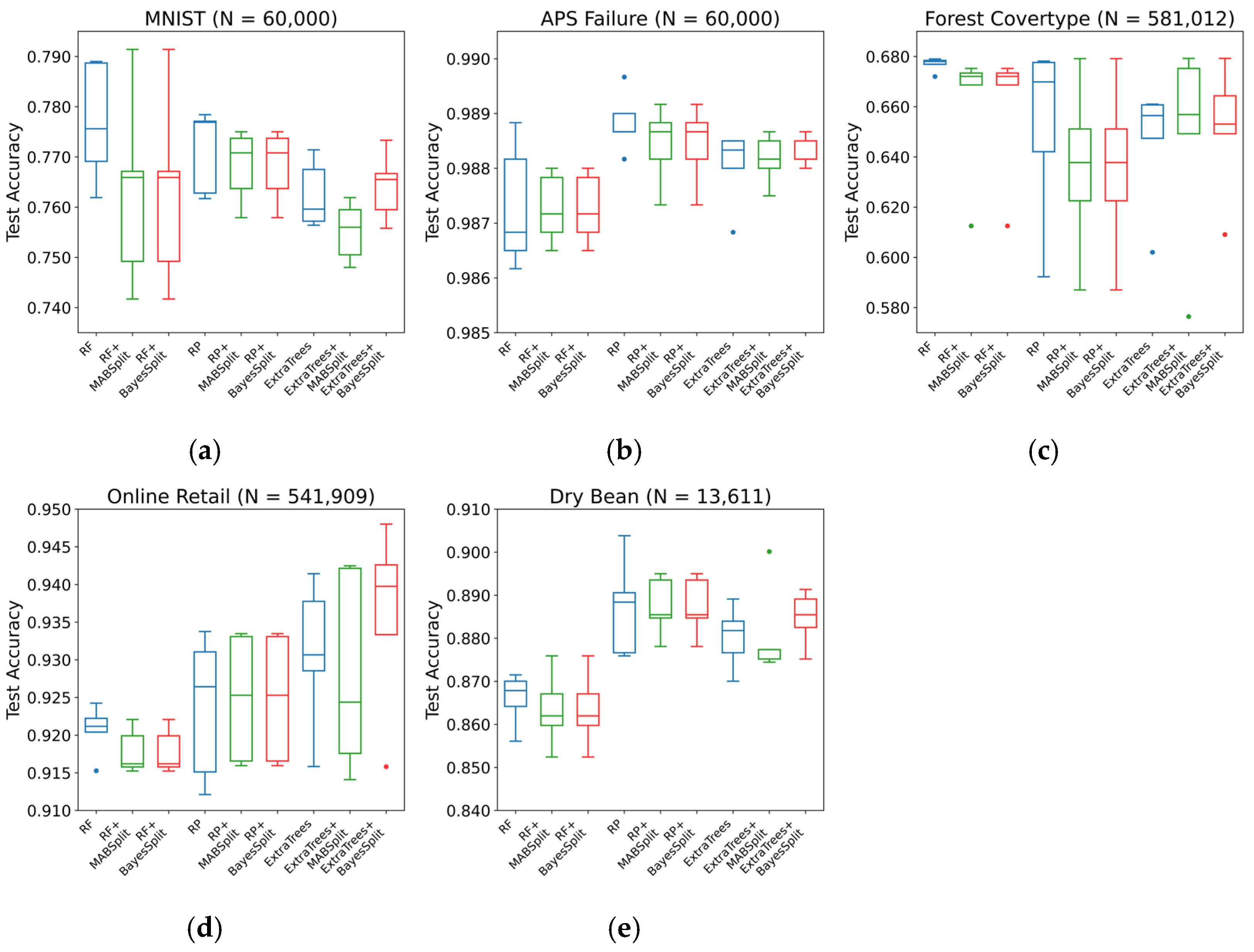
Classification: We assessed the performance of BayesSplit by comparing it with MABSplit and the baseline brute-force solver on several classification tasks, evaluating wall-clock training time, number of histogram insertions, and test accuracy. As shown in Figure 2, incorporating BayesSplit and MABSplit subroutines significantly reduces training time relative to the naïve approach, with BayesSplit providing up to a 95% reduction compared to baseline methods.
Table 2 further confirms their efficiency by showing fewer histogram insertions, with BayesSplit’s refined histogram-based splits providing additional computational savings to the ExtraTrees model. The identical insertion counts between BayesSplit and MABSplit for RF and RP models occur because both algorithms eliminate candidates at similar rates when significant differences in split quality are evident. Given the strong correlation between histogram insertions and training time, improving node-splitting by reducing sample complexity is clearly justified.
Figure 3 illustrates that integrating BayesSplit and MABSplit produces test accuracy comparable to that of the baseline models. Notably, BayesSplit provides significant advantages to the ExtraTrees model, which typically relies on random split thresholds that can lead to suboptimal decisions. Through Bayesian optimization, BayesSplit refines those random splits, resulting in more precise decision boundaries and improved accuracy.
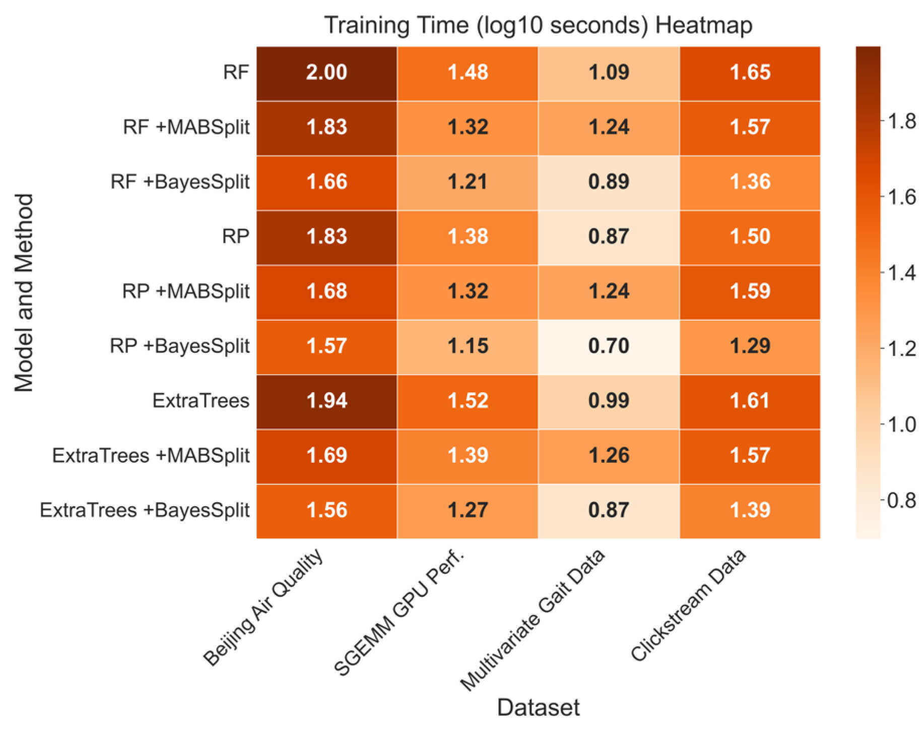
Regression: Across four regression datasets with diverse characteristics, BayesSplit consistently reduces training time by 20–70% compared to MABSplit, as shown in Figure 4. To ensure fairness given the varying histogram bin counts of the baseline regression models, we excluded the number of histogram insertions from our analysis.
Table 3 shows that using BayesSplit yields lower test MSEs than the naïve solver or MABSplit, and the improvement in generalization performance along with reduced training time highlights the effectiveness of Bayesian optimization in efficiently focusing on the most promising splits.

4.2. Fixed Budget Comparisons

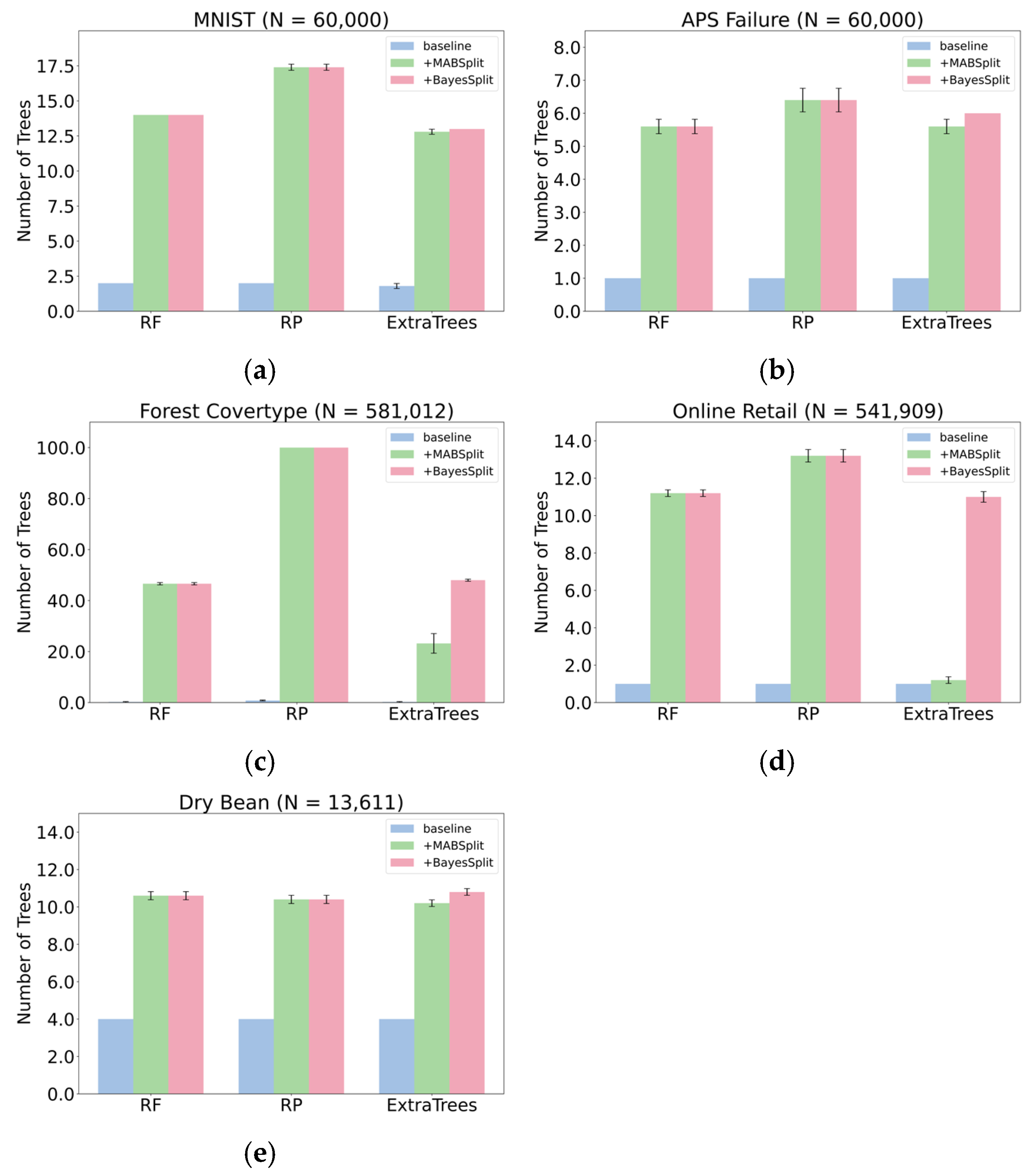
Classification: Under a fixed computational budget defined by a set number of histogram insertions, forests trained with BayesSplit split more nodes and require fewer data-point queries than those using the naïve solver. Consequently, these forests can accommodate more trees and achieve improved generalization.
Figure 5 compares the number of classification trees built under a fixed budget with test accuracies in Table 4. For RF and RP, BayesSplit and MABSplit perform similarly across all five datasets. However, in ExtraTrees, BayesSplit surpasses MABSplit in both tree count and test accuracy, indicating that BayesSplit effectively captures and leverages the additional randomness in ExtraTrees’ split-selection process.
Regression: Under a fixed computational budget, integrating BayesSplit consistently outperforms both the naïve approach and MABSplit, allowing more trees to be trained and yielding lower test MSEs in all baseline models. Figure 6 shows that BayesSplit supports additional regression trees within the same budget, and Table 5 confirms notable improvements in predictive performance via reduced test MSEs. Notably, compared to MABSplit, BayesSplit can reduce the test MSEs by up to 25%.
BayesSplit proves particularly well-suited to regression tasks due to the continuous nature of the target variable, which enables more precise estimation of impurity reductions. This precision results in tighter confidence intervals within the Bayesian updating framework, allowing the algorithm to allocate more samples to regions of high uncertainty while limiting evaluations in low-variance segments. Consequently, BayesSplit converges more rapidly toward optimal splits, reducing unnecessary computations and enhancing overall efficiency.

4.3. Feature Stability Comparisons

Beyond predictive performance, Random Forests offer valuable insights into feature importance, thereby enhancing model explainability [32]. We evaluate feature importance using two well-established metrics: Out-of-Bag Permutation Importance (OOB-PI) and Mean Decrease in Impurity (MDI). Specifically, OOB-PI quantifies the change in out-of-bag error when the values of a feature are shuffled, reflecting its contribution to predictive accuracy. On the other hand, MDI calculates the average reduction in impurity (e.g., Gini index or entropy for classification, MSE for regression) across all decision nodes where a given feature is used for splitting, indicating its effectiveness in reducing overall impurity within the model. To ensure robustness, the top   k   features identified by these metrics are further assessed for stability using standardized formulas [33].
Table 6 shows that under a fixed computational budget, forests trained with BayesSplit achieve a 10–40% improvement in feature stability compared to MABSplit, corresponding to an average increase of approximately 30.28%. This improvement is particularly significant in resource-constrained environments, such as IoT and edge computing applications, where model interpretability and robustness are critical. By consistently identifying the most relevant features across multiple iterations, BayesSplit not only enhances predictive performance but also mitigates the risk of overfitting to irrelevant or noisy data.

5. Conclusions and Future Work

In this work, the BayesSplit algorithm was proposed as a Bayesian enhancement of MABSplit for decision-tree node splitting. While MABSplit introduces multi-armed bandit techniques with frequentist confidence intervals, BayesSplit advances this approach by developing a Bayesian-based impurity estimation framework where impurity reduction events are treated as Bernoulli trials. On the benchmark datasets, BayesSplit reduced wall-clock training time by 20–70% relative to MABSplit and by up to 95% relative to the naïve approach. Compared to MABSplit, it also lowered regression MSEs by as much as 25%.
Beyond computational efficiency, BayesSplit exhibits enhanced feature stability. Our experiments primarily focused on standard computing environments, making it an important future research direction to benchmark and optimize BayesSplit for resource-constrained devices such as smartphones and IoT platforms. Given the growing relevance of edge computing, which involves limited memory, power constraints, and specialized hardware architectures, dedicated optimizations and platform-specific considerations are critical. Future work could also extend BayesSplit to parallel frameworks such as Apache Spark, further broadening its applicability in large-scale real-time processing scenarios.
Finally, we note that gradient boosting decision tree (GBDT) frameworks such as XGBoost, LightGBM, and CatBoost remain strong baselines in predictive performance. These boosting algorithms often achieve higher accuracy than bagging-based methods on many tasks due to their sequential error-correcting training process. In contrast, our work focuses on the Random Forest framework, where trees are constructed in parallel, aiming to improve training efficiency without sacrificing accuracy. Nevertheless, integrating BayesSplit’s adaptive splitting strategy into boosting frameworks offers potential advantages, such as selectively updating the necessary data points’ residual targets rather than recomputing residuals for the entire dataset at each iteration. Although such integration presents practical and algorithmic challenges, it represents a promising direction for future research, as indicated by recent advances such as FastForest [9]. Thus, our proposed approach complements rather than directly competes with optimized gradient boosting and hybrid methods. We intend to explore this topic in greater detail in future work.

Author Contributions

Conceptualization, J.H. and L.Y.; methodology, L.Y.; software, Z.L.; validation, Z.L.; formal analysis, Z.L.; investigation, J.H., L.Y. and Z.L.; resources, L.Y.; data curation, Z.L.; writing—original draft preparation, L.Y. and Z.L.; writing—review and editing, L.Y. and Z.L.; visualization, Z.L.; supervision, J.H. and L.Y.; project administration, J.H.; funding acquisition, L.Y. All authors have read and agreed to the published version of the manuscript.

Funding

This research was funded by the National Natural Science Foundation of China, under grant number [52307232], and the Hunan Provincial Natural Science Foundation of China, under grant number [2024JJ4055].

Data Availability Statement

The datasets analyzed during the current study are publicly available from the UCI Machine Learning Repository: https://archive.ics.uci.edu/ml/index.php (accessed on 31 May 2024).

Conflicts of Interest

The authors declare no conflicts of interest.

Appendix A

This section provides the complete derivation underlying Theorem 1.
Proof. 
To facilitate a deeper analysis of the result, we first introduce several key definitions. □
Definition A1.
(Quantities  k f t τ i τ S f t τ ,   μ f t ~ τ ).  k f t τ  denotes the number of times the feature–threshold pair  f , t  has been selected for evaluation up to computation step   τ i τ  represents the feature–threshold pair selected at computation step   τ , and  S f t τ  is the cumulative count of times that the pair  f , t  resulted in impurity reduction up to step   τ . For Bernoulli bandits in BayesSplit,  μ f t ~ τ    is calculated as  μ f t ~ τ = S f t τ k f t τ + 1 .
Definition A2. 
(Quantities  θ f t τ ).  θ f t τ  denotes a sample generated independently for each feature–threshold pair  f , t  from the posterior distribution at step  τ . In BayesSplit, this sample is drawn from the Beta distribution   B e t a S f t τ + 1 ,   k f t τ S f t τ + 1 .
Definition A3. 
(Quantities   x f t ,   y f t ). For each feature–threshold pair  f , t f b , t b , we define two thresholds  x f t  and  y f t  such that  p f t < x f t < y f t < p f b t b , their exact values depend on the context of the proof.
Definition A4. 
(Events   E f t μ τ ,   E f t θ τ ). For any  f , t f b , t b E f t μ τ  is the event that the empirical mean  μ f t ~ τ x f t , and  E f t θ τ  is the event that the sampled value  θ f t τ y f t .
Definition A5. 
(History  F τ ). For computation steps  τ = 1,2 , ,   define  F τ  as the history of all evaluations up to step  τ :
F τ = { i ( τ ) , r i ( τ ) ( τ ) ,   τ = 1 , τ }
where  i τ  denotes the feature–threshold pair selected at step  τ , and  r i τ τ  is the observed impurity reduction for that pair at step  τ .  whether or not the event  E f t μ τ   holds is determined by  F τ 1 .
Definition A6. 
(Probability   Ƥ f t , τ ). Define     Ƥ f t , τ   as the probability that   θ f b t b τ    exceeds     y f t   at computation step   τ :
Ƥ f t , τ = P r θ f b t b τ > y f t | F τ 1
where    Ƥ f t , τ   is a random variable determined by the history of previous evaluations  F τ 1 .
Now we proceed to establish the upper bound on regret in Theorem 1. We begin by decomposing the expected number of times a suboptimal pair  f , t f b , t b   is chosen, written as follows:
E k f t M = τ = 1 M P r i τ = f , t , E f t μ τ , E f t θ τ + τ = 1 M P r i τ = f , t , E f t μ τ , E f t θ τ ¯ + τ = 1 M P r i τ = f , t , E f t μ τ ¯
Each of these terms will be bounded separately. We start with the first term and introduce Lemma A1, which is addressed as follows:
Lemma A1. 
For all computation steps  τ , and for every feature–threshold pair  f , t f b , t b , given any history  F τ 1 , the following holds:
P r i τ = f , t , E f t μ τ , E f t θ τ | F τ 1 1 Ƥ f t , τ Ƥ f t , τ P r i τ = f b , t b , E f t μ τ , E f t θ τ | F τ 1
Proof. 
We aim to demonstrate that for any suboptimal pair  f , t f b , t b  and any history  F τ 1 :
P r i τ = f , t | E f t θ τ , F τ 1 1 Ƥ f t , τ Ƥ f t , τ P r i τ = f b , t b | E f t θ τ , F τ 1
We begin by observing that to make the event  E f t θ τ   stand,  i τ = f , t  only if  θ f t τ y f t  for any  f , t f b , t b ,   implying the following:
P r i τ = f , t | E f t θ τ , F τ 1 1 Ƥ f t , τ · P r θ f * t * τ y f t , f * , t * f b , t b | E f t θ τ , F τ 1
Similarly, for the optimal pair  f b , t b ,   we have the following:
P r i τ = f b , t b | E f t θ τ , F τ 1 Ƥ f t , τ · P r θ f * t * τ y f t , f * , t * f b , t b | E f t θ τ , F τ 1
By combining the above two inequalities, we obtain the desired result. □
Applying Lemma A1 to the first term of Equation (A1), we obtain the following:
τ = 1   M P r i τ = f , t , E f t μ τ , E f t θ τ = τ = 1 M E P r i τ = f , t , E f t μ τ , E f t θ τ | F τ 1 = τ = 1 M E 1 Ƥ f t , τ Ƥ f t , τ I i τ = f b , t b , E f t μ τ , E f t θ τ
Lemma A2. 
For any feature–threshold pair  f , t f b , t b  we calculate the following:
τ = 1 M P r i τ = f , t , E f t μ τ , E f t θ τ 24 f t 2 + j 8 f t Θ e x p f t 2 j / 2 + 1 j + 1 f t 2 e x p D f t j + 1 e x p f t 2 j / 4 1  
where  f t = p f b t b y f t  and  D f t = y f t ln y f t p f b t b + 1 y f t ln 1 y f t 1 p f b t b .
Proof. 
To prove the bound in Equation (A3), we first note that the expression  E 1 Ƥ f t , τ Ƥ f t , τ   can be decomposed based on when the optimal feature–threshold pair   f b , t b   is chosen. Let   τ j   denote the computation step at which the optimal pair   f b , t b   is evaluated for the   j -th time. Then we obtain the following:
τ = 1 M E 1 Ƥ f t , τ Ƥ f t , τ I i τ = f b , t b , E f t μ τ , E f t θ τ j = 0 M 1 E 1 Ƥ f t , τ j + 1 1
For small values of  j < 8 / f t , we can bound  E 1 Ƥ f t , τ j + 1 1 3 f t . This contributes a total of  24 f t 2   to the bound since there are at most  8 f t   such terms.
For larger values of  j 8 / f t , the posterior distribution for the optimal pair   f b , t b   becomes more concentrated as more evaluations are performed. Using properties of the Beta distribution and KL divergence,  E 1 Ƥ f t , τ j + 1 1   decreases at a rate determined by three components. The first component of the bound  e x p f t 2 j / 2   arises from applying Chernoff–Hoeffding bound [34] to the concentration of the posterior mean around the true impurity reduction probability. This term captures how quickly the algorithm’s beliefs about the quality of the optimal split converge as more samples are collected. The second component  1 j + 1 f t 2 e x p D f t j   emerges from a more refined analysis using the KL divergence   D f t   between the impurity reduction probabilities. The last component  1 e x p f t 2 j / 4 1   handles the tail probabilities when considering the TS procedure’s random draws from posterior distributions, showing that the probability of selecting a suboptimal split diminishes rapidly with additional evidence.
The detailed proof involves various technical assumptions and numerical estimates, so we opt for a simplified approach. □
To finish handling the last two terms in Equation (A1), we introduce additional lemmas.
Lemma A3. 
For any feature–threshold pair  f , t f b , t b  the following is calculated:
τ = 1 M P r i τ = f , t , E f t μ τ ¯ 1 d x f t , p f t + 1
Proof. 
Let  τ k  be the computation step for the  k -th trial of  f , t . Recall that the event  E f t μ τ ¯  corresponds to  μ f t ~ τ > x f t , we obtain the following:
τ = 1 M P r i τ = f , t , E f t μ τ ¯ k = 0 M 1 P r E f t μ τ k + 1 ¯
In BayesSplit, the empirical mean  μ f t ~ τ k + 1  at computation step  τ k + 1  depends on the cumulative outcomes of  k  i.i.d. evaluations of the arm  f , t . That is,  μ f t ~ τ k + 1 = S f t τ k + 1 k + 1 . By applying the Chernoff–Hoeffding bound, we derive  P r S f t τ k + 1 k + 1 > x f t P r S f t τ k + 1 k > x f t e x p k d x f t , p f t , leading to the following:
k = 0 M 1 P r E f t μ τ k + 1 ¯ = k = 0 M 1 P r μ f t ~ τ k + 1 > x f t 1 + k = 1 M 1 e x p k d x f t , p f t 1 + 1 d x f t , p f t
where  d x f t , p f t > 0 . This completes the proof of Lemma A3. □
Lemma A4. 
For any feature–threshold pair  f , t f b , t b  the following is calculated.
τ = 1 M P r i τ = f , t , E f t μ τ , E f t θ τ ¯ L f t M + 1
where  L f t M = ln M d x f t , y f t .
Proof. 
We divide the summation of probabilities into two cases, depending on whether the number of selections for   f , t , denoted  k f t τ , is less than or exceeds   L f t M .
τ = 1 M P r i τ = f , t , E f t μ τ , E f t θ τ ¯ = τ = 1 M P r i τ = f , t , k f t τ L f t M , E f t μ τ , E f t θ τ ¯ + τ = 1 M P r i τ = f , t , k f t τ > L f t M , E f t μ τ , E f t θ τ ¯
For the case where  k f t τ L f t M , the sum is trivially bounded by   L f t M . Now we handle the case where  k f t τ > L f t M . Once   k f t τ  is large, and the event  E f t μ τ  holds, the probability that  E f t θ τ  fails to hold becomes small.   θ f t τ  follows a Beta distribution with parameters  μ f t ~ τ  and  k f t τ :
θ f t τ ~ B e t a μ f t ~ τ k f t τ + 1 + 1 , 1 μ f t ~ τ k f t τ + 1
and the sum of these parameters is given by  s = α + β = k f t τ + 2 . By leveraging the monotonicity property of the KL divergence and the fact that  p f t < x f t < y f t , we relate the divergence  d p f t , y f t  to  d x f t , y f t . This relationship allows us to assert that the probability of  θ f t τ > y f t  decreases exponentially with respect to  s  and the divergence  d x f t , y f t . We obtain the following upper bound on the tail probability:
P r θ f t τ > y f t | F τ 1 e x p k f t τ + 2 d x f t , y f t
Under the condition that  k f t τ > L f t M , a simplified inequality is given by the following equation:
e x p k f t τ + 2 d x f t , y f t e x p L f t M d x f t , y f t = 1 M
Hence, for any history  F τ 1 , we conclude the following equation:
P r θ f t τ > y f t | F τ 1 1 M
Summing over all computation steps, the second term is bounded by 1. □
By combining the results of prior derivations, we obtain an upper bound on the expected number of times a suboptimal feature–threshold pair  f , t f b , t b  is chosen during  M  computational steps:
E k f t M 24 f t 2 + j 8 / f t Θ e x p f t 2 j / 2 + 1 j + 1 f t 2 e x p D f t j + 1 e x p f t 2 j / 4 1   + L f t M + 1 + 1 + 1 d x f t , p f t
To derive the BayesSplit-specific bound, we set  0 < ϵ 1  and  x f t p f t , p f b t b  such that   d x f t , p f b t b = d p f t , p f b t b / 1 + ϵ .   Similarly,  y f t x f t , p f b t b   and this gives  d x f t , y f t = d x f t , p f b t b / 1 + ϵ . We then obtain the following:
L f t M = ln M d x f t , y f t = 1 + ϵ 2 ln M d p f t , p f b t b
and by straightforward algebraic manipulation of the divergence   d x f t , p f t , we arrive at the following:
1 d x f t , p f t 1 2 x f t p f t 2 = O 1 ϵ 2
Putting all the results together yields the following:
E k f t M 24 f t 2 + Θ 1 f t 2 + 1 f t 2 D f t + 1 f t 4 + 1 + ϵ 2 ln M d p f t , p f b t b + O 1 ϵ 2 = O 1 + 1 + ϵ 2 ln M d p f t , p f b t b + O 1 ϵ 2
which simplifies to a big-Oh expression. Finally, we combine all suboptimal pairs to arrive at the expected regret bound for BayesSplit:
E R M = f , t f t E k f t M f , t 1 + ϵ 2 ln M d p f t , p f b t b f t + O m T ϵ 2
In practice, relying on posterior means and confidence intervals for feature–threshold selection reduces exploration relative to purely random sampling. Nevertheless, our experiments show that this trade-off preserves low regret while delivering significant computational speedups. □

Appendix B

In this section, we conducted additional experiments evaluating BayesSplit’s sensitivity to hyperparameter settings and its performance on imbalanced datasets.

Appendix B.1. Sensitivity to Hyperparameter Settings

We examined BayesSplit’s sensitivity to prior initialization and key hyperparameters, including batch size and histogram bins. All experiments in this section were conducted using Random Forest integrated with BayesSplit.
Prior Settings: Table A1 presents the impact of different Beta prior initializations on BayesSplit performance. We tested symmetric priors ( B e t a 1,1   and   B e t a 2,2 ) and asymmetric priors ( B e t a 1,2   and   B e t a 2,1 ) on both classification and regression tasks. The results demonstrate remarkable stability across all prior settings, with virtually identical test performance metrics. These findings empirically validate our theoretical framework described in Section 3.2, where the initialization provides an informed starting point, but its influence diminishes as more batches are processed, with split selection ultimately determined by empirical evidence rather than prior assumptions.
Table A1. Impact of different prior settings on BayesSplit performance.
DatasetPrior SettingTraining Time (s)Performance
Metric
Test Performance
Online retail
(Classification)
Beta (1,1)6.552   ±   0.786Accuracy0.918   ±   0.001
Beta (2,2)6.214   ±   1.277Accuracy0.918   ±   0.001
Beta (1,2)5.221   ±   0.096Accuracy0.918   ±   0.001
Beta (2,1)5.421   ±   0.331Accuracy0.918   ±   0.001
SGEMM GPU kernel performance
(Regression)
Beta (1,1)19.436   ±   1.829MSE27,957.258   ±   395.620
Beta (2,2)21.017   ±   2.126MSE27,957.258   ±   395.620
Beta (1,2) 20.287   ±   0.186MSE27,957.258   ±   395.620
Beta (2,1)20.649   ±   0.231MSE27,957.258   ±   395.620
Batch Size and Histogram Bins: Table A2 investigates the sensitivity to batch size and histogram bin configuration. Our experiments maintain consistency with MABSplit’s default settings (batch size = 1000, histogram bins = 11) as the baseline. Varying batch sizes from 500 to 1500 show minimal impact on accuracy, with all configurations achieving over 91% accuracy. Notably, increasing histogram bins to 20 yields the best performance (93.1–93.3% accuracy). This performance gain can be attributed to the increased resolution in feature space partitioning, enabling more precise identification of optimal split thresholds. The robustness across different batch sizes indicates that BayesSplit efficiently utilizes samples regardless of batching strategy.
Table A2. Impact of batch size and histogram bins on BayesSplit performance (online retail).
Online Retail Dataset (N = 541,909)
Histogram Bins = 5Histogram Bins = 11Histogram Bins = 20
Batch SizeTime (s)Accuracy (%)Time (s)Accuracy (%)Time (s)Accuracy (%)
5005.729   ±   0.79491.316   ±   0.0017.321   ±   0.89391.544   ±   0.0026.069   ±   0.23093.109   ±   0.001
10007.328   ±   0.95991.317   ±   0.0017.201   ±   1.11991.785   ±   0.0016.267   ±   0.10193.258   ±   0.001
15004.997   ±   0.24191.356   ±   0.0017.548   ±   0.37491.664   ±   0.0027.646   ±   0.23492.700   ±   0.002

Appendix B.2. Performance on Imbalanced Dataset

To evaluate BayesSplit’s robustness on imbalanced data, we utilized the Online Shoppers Purchasing Intention dataset from the UCI repository, which exhibits significant class imbalance with only 15.5% positive class samples (customers who made purchases) versus 84.5% negative samples (non-purchasing visitors).
The results in Table A3 demonstrate that BayesSplit maintains competitive accuracy while significantly reducing training time across all baseline models. In these models, ExtraTrees+BayesSplit achieves comparable accuracy (88.483%) to the baseline (88.451%) while reducing training time by 47.6%. These results indicate that BayesSplit’s adaptive splitting strategy effectively handles class imbalance by focusing computational resources on informative splits rather than exhaustively evaluating all candidates, making it suitable for real-world applications where class imbalance is common.
Table A3. Training time and test accuracies for models with and without BayesSplit on an imbalanced dataset.
Online Shoppers Purchasing Intention Dataset (N = 12,330, Maximum Depth = 5)
ModelTraining Time (s)Test Accuracy (%)
RF11.028   ±   0.95188.694   ±   0.001
RF+BayesSplit6.112   ± 0.44188.111   ± 0.002
RP6.320   ±   0.21688.369   ±   0.003
RP+BayesSplit3.547   ± 0.07087.672   ± 0.003
ExtraTrees11.206   ±   1.28388.451   ±   0.002
ExtraTrees+BayesSplit5.876   ± 0.83488.483   ± 0.003

References

  1. Adnan, M.N.; Islam, M.Z. Optimizing the Number of Trees in a Decision Forest to Discover a Subforest with High Ensemble Accuracy Using a Genetic Algorithm. Knowl.-Based Syst. 2016, 110, 86–97. [Google Scholar] [CrossRef]
  2. Breiman, L. Random Forests. Mach. Learn. 2001, 45, 5–32. [Google Scholar] [CrossRef]
  3. Ngo, G.; Beard, R.; Chandra, R. Evolutionary Bagging for Ensemble Learning. Neurocomputing 2022, 510, 1–14. [Google Scholar] [CrossRef]
  4. Abellán, J.; Mantas, C.J.; Castellano, J.G. A Random Forest Approach Using Imprecise Probabilities. Knowl.-Based Syst. 2017, 134, 72–84. [Google Scholar] [CrossRef]
  5. Zhang, X.; Lin, X.; Zhao, J.; Huang, Q.; Xu, X. Efficiently Predicting Hot Spots in PPIs by Combining Random Forest and Synthetic Minority Over-Sampling Technique. IEEE/ACM Trans. Comput. Biol. Bioinf. 2018, 16, 774–781. [Google Scholar] [CrossRef] [PubMed]
  6. Jiang, N.; Sheng, B.; Li, P.; Lee, T.Y. PhotoHelper: Portrait Photographing Guidance via Deep Feature Retrieval and Fusion. IEEE Trans. Multimed. 2022, 25, 2226–2238. [Google Scholar] [CrossRef]
  7. Yin, L.; Li, B.; Li, P.; Zhang, R. Research on Stock Trend Prediction Method Based on Optimized Random Forest. CAAI Trans. Intell. Technol. 2023, 8, 274–284. [Google Scholar] [CrossRef]
  8. Wang, X.; Du, S.; Feng, C.C.; Zhang, X.; Zhang, X. Interpreting the Fuzzy Semantics of Natural-Language Spatial Relation Terms with the Fuzzy Random Forest Algorithm. ISPRS Int. J. Geo-Inf. 2018, 7, 58. [Google Scholar] [CrossRef]
  9. Yates, D.; Islam, M.Z. FastForest: Increasing Random Forest Processing Speed While Maintaining Accuracy. Inf. Sci. 2021, 557, 130–152. [Google Scholar] [CrossRef]
  10. Dinh, T.P.; Pham-Quoc, C.; Thinh, T.N.; Do Nguyen, B.K.; Kha, P.C. A Flexible and Efficient FPGA-Based Random Forest Architecture for IoT Applications. Internet Things 2023, 22, 100813. [Google Scholar] [CrossRef]
  11. Sun, Z.; Wang, G.; Li, P.; Wang, H.; Zhang, M.; Liang, X. An Improved Random Forest Based on the Classification Accuracy and Correlation Measurement of Decision Trees. Expert Syst. Appl. 2024, 237, 121549. [Google Scholar] [CrossRef]
  12. Ma, J.; Pan, Q.; Guo, Y. Depth-First Random Forests with Improved Grassberger Entropy for Small Object Detection. Eng. Appl. Artif. Intell. 2022, 114, 105138. [Google Scholar] [CrossRef]
  13. Chen, J.; Wang, X.; Lei, F. Data-Driven Multinomial Random Forest: A New Random Forest Variant with Strong Consistency. J. Big Data 2024, 11, 34. [Google Scholar] [CrossRef]
  14. Qiu, Y.; Zhou, J.; Khandelwal, M.; Yang, H.; Yang, P.; Li, C. Performance Evaluation of Hybrid WOA-XGBoost, GWO-XGBoost and BO-XGBoost Models to Predict Blast-Induced Ground Vibration. Eng. Comput. 2022, 38, 4145–4162. [Google Scholar] [CrossRef]
  15. Punmiya, R.; Choe, S. Energy Theft Detection Using Gradient Boosting Theft Detector with Feature Engineering-Based Preprocessing. IEEE Trans. Smart Grid 2019, 10, 2326–2329. [Google Scholar] [CrossRef]
  16. Herrera, V.M.; Khoshgoftaar, T.M.; Villanustre, F.; Furht, B. Random Forest Implementation and Optimization for Big Data Analytics on LexisNexis’s High Performance Computing Cluster Platform. J. Big Data 2019, 6, 1–36. [Google Scholar] [CrossRef]
  17. Chen, J.; Li, K.; Tang, Z.; Bilal, K.; Yu, S.; Weng, C.; Li, K. A Parallel Random Forest Algorithm for Big Data in a Spark Cloud Computing Environment. IEEE Trans. Parallel Distrib. Syst. 2017, 28, 919–933. [Google Scholar] [CrossRef]
  18. Domingos, P.; Hulten, G. Mining High-Speed Data Streams. In Proceedings of the 6th ACM SIGKDD International Conference on Knowledge Discovery and Data Mining, Boston, MA, USA, 20–23 August 2000; pp. 71–80. [Google Scholar] [CrossRef]
  19. Manapragada, C.; Webb, G.I.; Salehi, M. Extremely Fast Decision Tree. In Proceedings of the 24th ACM SIGKDD International Conference on Knowledge Discovery and Data Mining, London, UK, 19–23 August 2018; pp. 1953–1962. [Google Scholar] [CrossRef]
  20. Mu, Y.; Liu, X.; Wang, L. A Pearson’s Correlation Coefficient Based Decision Tree and Its Parallel Implementation. Inf. Sci. 2018, 435, 40–58. [Google Scholar] [CrossRef]
  21. Xu, Y. Research and Implementation of Improved Random Forest Algorithm Based on Spark. In Proceedings of the 2nd IEEE International Conference on Big Data Analytics, Chengdu, China, 18–19 October 2017; pp. 499–503. [Google Scholar] [CrossRef]
  22. Yin, L.; Chen, K.; Jiang, Z.; Xu, X. A Fast Parallel Random Forest Algorithm Based on Spark. Appl. Sci. 2023, 13, 6121. [Google Scholar] [CrossRef]
  23. Tiwari, M.; Kang, R.; Lee, J.; Piech, C.; Shomorony, I.; Thrun, S.; Zhang, M.J. MABSplit: Faster Forest Training Using Multi-Armed Bandits. In Proceedings of the Advances in Neural Information Processing Systems, New Orleans, LA, USA, 6–12 December 2022; Volume 35, pp. 1223–1237. [Google Scholar]
  24. Li, X.; Wang, Y.; Basu, S.; Kumbier, K.; Yu, B. A Debiased MDI Feature Importance Measure for Random Forests. In Proceedings of the Advances in Neural Information Processing Systems, Vancouver, BC, Canada, 8–14 December 2019; Volume 32, pp. 8049–8059. [Google Scholar] [CrossRef]
  25. Breiman, L.; Friedman, J.H.; Olshen, R.A.; Stone, C.J. Classification and Regression Trees; Routledge: New York, NY, USA, 2017. [Google Scholar]
  26. Russo, D.; Van Roy, B. Learning to Optimize via Posterior Sampling. Math. Oper. Res. 2014, 39, 1221–1243. [Google Scholar] [CrossRef]
  27. Zhu, Z.; Huang, L.; Xu, H. Self-Accelerated Thompson Sampling with Near-Optimal Regret Upper Bound. Neurocomputing 2020, 399, 37–47. [Google Scholar] [CrossRef]
  28. Russo, D.; Van Roy, B.; Kazerouni, A.; Osband, I.; Wen, Z. A Tutorial on Thompson Sampling. Found. Trends Mach. Learn. 2018, 11, 1–96. [Google Scholar] [CrossRef]
  29. Agahi, H. A Modified Kullback–Leibler Divergence for Non-Additive Measures Based on Choquet Integral. Fuzzy Sets Syst. 2019, 367, 107–117. [Google Scholar] [CrossRef]
  30. Saeed, U.; Jan, S.U.; Lee, Y.D.; Koo, I. Fault Diagnosis Based on Extremely Randomized Trees in Wireless Sensor Networks. Reliab. Eng. Syst. Saf. 2021, 205, 107284. [Google Scholar] [CrossRef]
  31. Gomes, H.M.; Read, J.; Bifet, A.; Durrant, R.J. Learning from Evolving Data Streams Through Ensembles of Random Patches. Knowl. Inf. Syst. 2021, 63, 1597–1625. [Google Scholar] [CrossRef]
  32. Alduailij, M.; Khan, Q.W.; Tahir, M.; Sardaraz, M.; Alduailij, M.; Malik, F. Machine-Learning-Based DDoS Attack Detection Using Mutual Information and Random Forest Feature Importance Method. Symmetry 2022, 14, 1095. [Google Scholar] [CrossRef]
  33. Nogueira, S.; Sechidis, K.; Brown, G. On the Stability of Feature Selection Algorithms. J. Mach. Learn. Res. 2018, 18, 1–54. [Google Scholar]
  34. Hellman, M.; Raviv, J. Probability of Error, Equivocation, and the Chernoff Bound. IEEE Trans. Inf. Theory 1970, 16, 368–372. [Google Scholar] [CrossRef]
Figure 1. BayesSplit framework workflow.
Make 07 00070 g001
Figure 2. Classification wall-clock training time.
Make 07 00070 g002
Figure 3. Classification test accuracy on different datasets. (a) MNIST dataset (N = 60,000); (b) APS Failure dataset (N = 60,000); (c) Forest Covertype dataset (N = 581,012); (d) Online Retail dataset (N = 541,909); (e) Dry Bean dataset (N = 13,611).
Make 07 00070 g003
Figure 4. Regression wall-clock training time.
Make 07 00070 g004
Figure 5. Number of classification trees under a fixed computational budget on different datasets. (a) MNIST dataset (N = 60,000); (b) APS Failure dataset (N = 60,000); (c) Forest Covertype dataset (N = 581,012); (d) Online Retail dataset (N = 541,909); (e) Dry Bean dataset (N = 13,611).
Make 07 00070 g005
Figure 6. Number of regression trees under a fixed computational budget on different datasets. (a) Beijing Air Quality dataset (N = 420,768); (b) SGEMM GPU Perf. dataset (N = 241,600); (c) Multivariate Gait Data dataset (N = 181,800); (d) Clickstream Data dataset (N = 165,474).
Make 07 00070 g006
Table 1. Notations in BayesSplit algorithm and analysis.
SymbolMeaning
  D   dataset   with   N   data   points   x i , y i i = 1 N
  N total number of data points
  x i i -th feature vector
  y i   target   value   corresponding   to   x i
  R ν region in feature space corresponding to node   ν  
  N n ν number of samples falling into region   R ν  
  M set of features considered for splitting
  T set of possible thresholds for each feature
  f , t feature–threshold pair (candidate split)
  I · impurity measure (Gini index, entropy, or MSE)
  μ f t   optimization   objective   for   split   f , t
  μ ^ f t point   estimate   of   μ f t   from histogram
  n number of subsamples for confidence interval estimation
  C f t n , δ confidence interval width with confidence level   1 δ  
  S s o l u t i o n set of candidate splits maintained by algorithm
  α , β parameters of Beta distribution
  g f t impurity gain
  μ ^ p o s t , f t   posterior   mean :   μ ^ p o s t , f t = α / α + β
  C p o s t , f t posterior confidence interval half-width
  B batch size for data sampling
  θ * true   probability   that   split   f , t   reduces impurity
Table 2. Number of histogram insertions for classification models.
Dataset
MNISTAPS FailureForest CovertypeOnline RetailDry Bean
RF1.54 × 108   ±  3.16 × 1051.88 × 107   ±  2.19 × 1041.04 × 108   ±   1.16 × 1053.60 × 107   ±   1.17 × 1051.21 × 106   ±   1.09 × 10³
RF+MABSplit3.93 × 106   ±  5.64 × 1037.85 × 105   ±  1.43 × 1041.04 × 106   ±  1.26 × 1043.68 × 105   ±  7.62 × 1034.00 × 105   ±   1.01 × 10⁴
RF+BayesSplit3.93 × 106   ±   5.64 × 1037.85 × 105   ±   1.43 × 1041.04 × 106   ±   1.26 × 1043.68 × 105   ±   7.62 × 1034.00 × 105   ±   1.01 × 10⁴
RP1.32 × 108   ±  6.95 × 1051.61 × 107   ±  3.52 × 1047.79 × 107   ±  4.95 × 1052.68 × 107   ±   1.50 × 1051.22 × 106   ±   1.65 × 10³
RP+MABSplit3.17 × 106   ±  1.40 × 1046.44 × 105   ±  2.43 × 1043.59 × 105   ±   1.71 × 1042.74 × 105   ±  1.48 × 1044.07 × 105   ±   2.31 × 10³
RP+BayesSplit3.17 × 106   ±   1.40 × 1046.44 × 105   ±   2.43 × 1043.59 × 105   ±   1.71 × 1042.74 × 105   ±   1.48 × 1044.07 × 105   ±   2.31 × 10³
ExtraTrees1.68 × 108   ±  0.00 × 1001.89 × 107   ±  3.85 × 1021.04 × 108   ±   1.29 × 1053.55 × 107   ±   2.12 × 1051.22 × 106   ±   1.91 × 10³
ExtraTrees+MABSplit4.32 × 106   ±  7.69 × 1038.03 × 105   ±  2.45 × 1042.24 × 106   ±   8.11 × 1056.12 × 106   ±   9.15 × 1054.15 × 105   ±   1.30 × 10⁴
ExtraTrees+BayesSplit4.32 × 106   ±   1.11 × 1047.43 × 105   ±   1.30 × 1041.00 × 106   ±   3.22 × 1043.63 × 105   ±   6.03 × 1033.87 × 105   ±   3.85 × 10³
Table 3. Regression test MSEs.
Dataset
Beijing Multi-Site Air QualitySGEMM GPU Kernel PerformanceMultivariate Gait DataClickstream Data
RF 1138.284   ±   4.066 28 , 822.531   ±   13.386 66.477   ±   0.066 10.399   ±   0.014
RF+MABSplit1132.521   ±   5.659 27 , 646.146   ±   391.684 51.270   ±   3.056 10.083   ±   0.136
RF+BayesSplit1113.040   ±   4.89827,957.258   ±   395.62039.888   ±   1.5399.193   ±   0.265
RP 889.993   ±   7.186 41 , 998.543   ±   5321.693 61.942   ±   6.699 7.656   ±   0.395
RP+MABSplit 861.830   ±   4.373 41 , 998.543   ±   5321.693 60.756   ±   7.296 7.490   ±   0.412
RP+BayesSplit856.503   ±   5.04141,964.334   ±   5267.32860.349   ±   6.0657.391   ±   0.422
ExtraTrees 829.345   ±   8.158 28 , 827.176   ±   20.081 37.568   ±   0.809 6.101   ±   0.155
ExtraTrees+MABSplit 824.230   ±   6.631 28 , 838.510   ±   0.143 35.958   ±   0.805 6.068   ±   0.103
ExtraTrees+BayesSplit818.699   ±   4.05927,953.338   ±   405.54634.857   ±   1.0536.312   ±   0.096
Table 4. Classification test accuracy (fixed computational budget).
Dataset
MNISTAPS FailureForest CovertypeOnline RetailDry Bean
RF0.575   ±   0.0060.983   ±   0.00.374   ±   0.0190.893   ±   0.0030.858   ±   0.003
RF+MABSplit0.825   ±   0.0010.987   ±   0.00.670   ±   0.0010.917   ±   0.0010.867   ±   0.002
RF+BayesSplit0.825   ±   0.0010.987   ±   0.00.670   ±   0.0010.917   ±   0.0010.867   ±   0.002
RP0.589   ±   0.0140.984   ±   0.00.553   ±   0.050.893   ±   0.0030.876   ±   0.001
RP+MABSplit0.834   ±   0.0010.988   ±   0.00.676   ±   0.0010.929   ±   0.0040.882   ±   0.002
RP+BayesSplit0.834   ±   0.0010.988   ±   0.00.676   ±   0.0010.929   ±   0.0040.882   ±   0.002
ExtraTrees0.563   ±   0.0080.983   ±   0.00.389   ±   0.0220.896   ±   0.0030.877   ±   0.004
ExtraTrees+MABSplit0.814   ±   0.0020.988   ±   0.00.653   ±   0.0140.919   ±   0.0080.885   ±   0.004
ExtraTrees+BayesSplit0.820   ±   0.0020.989   ±   0.00.672   ±   0.0010.933   ±   0.0050.887   ±   0.002
Table 5. Regression test MSEs (fixed computational budget).
Dataset
Beijing Multi-Site Air QualitySGEMM GPU Kernel PerformanceMultivariate Gait DataClickstream Data
RF 1150.986   ±   1.360 33 , 133.193   ±   229.830 109.821   ±   0.178 17.198   ±   0.013
RF+MABSplit1122.964   ±   0.636 27 , 539.144   ±   188.497 53.366   ±   2.076 10.176   ±   0.096
RF+BayesSplit1106.436   ±   0.36527,421.693   ±   98.70539.960   ±   0.4579.017   ±   0.070
RP 1169.343   ±   1.107 73 , 717.816   ±   4059.742 85.964   ±   3.780 13.117   ±   0.820
RP+MABSplit 1169.573   ±   3.351 70 , 140.627   ±   3425.126 76.579   ±   2.672 6.755   ±   0.192
RP+BayesSplit1135.562   ±   1.28167,814.118   ±   755.37870.194   ±   4.2036.678   ±   0.062
ExtraTrees 951.450   ±   1.656 33 , 104.573   ±   213.766 90.886   ±   1.426 13.004   ±   2.393
ExtraTrees+MABSplit 797.448   ±   1.581 28 , 969.467   ±   41.929 43.639   ±   2.203 6.087   ±   0.078
ExtraTrees+BayesSplit772.231   ±   0.92227,762.501   ±   136.81933.776   ±   0.4905.855   ±   0.048
Table 6. Stability scores (fixed computational budget).
ModelStability MetricDatasetStability
RF
RF+MABSplit
RF+BayesSplit
MDI
MDI
MDI
Random Classification
0.536   ±   0.039
0.863   ±   0.016
0.863   ±   0.016
RF
RF+MABSplit
RF+BayesSplit
MDI
MDI
MDI
Random Regression
Random Regression
Random Regression
0.497   ±   0.046
0.581   ±   0.050
0.805   ±   0.012
RF
RF+MABSplit
RF+BayesSplit
Permutation
Permutation
Permutation
Random Classification
0.599   ±   0.022
0.695   ±   0.025
0.787   ±   0.024
RF
RF+MABSplit
RF+BayesSplit
Permutation
Permutation
Permutation
Random Regression
Random Regression
Random Regression
0.403   ±   0.047
0.456   ±   0.041
0.634   ±   0.014
Disclaimer/Publisher’s Note: The statements, opinions and data contained in all publications are solely those of the individual author(s) and contributor(s) and not of MDPI and/or the editor(s). MDPI and/or the editor(s) disclaim responsibility for any injury to people or property resulting from any ideas, methods, instructions or products referred to in the content.

