1. Introduction
Traffic congestion presents a persistent and significant challenge in urban environments, resulting in adverse economic and social impacts, such as prolonged travel times, increased fuel consumption, and elevated air pollution levels. A primary contributor to this issue is the inefficiency of traffic signal control at urban intersections. In Vietnam, the problem is exacerbated by rapid urbanization and the continuous growth in private vehicle ownership, placing increasing pressure on transportation infrastructure. This trend is observed not only in major metropolitan areas, like Hanoi and Ho Chi Minh City, but also in smaller, well-planned cities, such as Danang. According to the General Statistics Office’s Population and Housing Census 2019 [
1], Danang ranked second nationwide in car ownership, with 10.7% of households owning a vehicle, second only to Hanoi. As one of the most dynamic and systematically planned cities in Vietnam, Danang is now experiencing worsening traffic congestion, underscoring the urgent need for effective traffic signal control strategies.
Conventional traffic signal control methods are widely implemented across global urban networks, including in Vietnam. These methods typically rely on fixed-time schedules [
2,
3,
4] or traffic-responsive control schemes [
5,
6]. Signal timings are often pre-configured based on historical traffic patterns or vehicle counts during peak hours. While these approaches are cost-effective, simple to implement, and adequate under stable traffic conditions, they lack the flexibility to respond to dynamic and unpredictable traffic fluctuations caused by incidents or surges in demand. Moreover, as urban traffic systems grow more complex, traditional control strategies often fall short in terms of scalability and optimization.
To address these limitations, Adaptive Traffic Signal Control (ATSC) systems have emerged as a promising alternative, receiving growing attention for their ability to reduce congestion and improve vehicle flow through real-time optimization [
7,
8,
9]. A variety of computational intelligence techniques have been employed to enhance ATSC, including genetic algorithms, swarm intelligence, and, notably, reinforcement learning (RL) [
10,
11,
12]. Among these, RL offers significant advantages due to its ability to learn from environmental feedback and make real-time adjustments to traffic signals. Several studies have shown that RL algorithms can effectively manage traffic flow at intersections by continuously updating decision policies based on real-world data [
13,
14,
15,
16]. RL is particularly well-suited for large-scale, interconnected traffic networks, offering the ability to coordinate multiple intersections. Moreover, it does not require prior assumptions about the traffic system’s structure, making it highly adaptable. However, RL methods are often hindered by the “curse of dimensionality”, which can degrade performance in complex or large-scale scenarios [
17].
To overcome these challenges, Deep Reinforcement Learning (DRL)—which combines the representational power of deep learning with RL’s decision-making capabilities—has been introduced. DRL leverages neural networks to approximate value functions and policy mappings in environments with large state and action spaces, making it increasingly prevalent in traffic signal control research [
18,
19,
20,
21,
22,
23,
24,
25]. Recent studies have focused on enhancing the adaptability of DRL models to dynamic traffic conditions. For example, Zhang et al. [
26] developed RL models that effectively learn and adapt to changing traffic environments, while Wei et al. [
27] proposed a deep Q-learning-based approach tested under realistic conditions. These methods typically employ deep neural networks (DNNs) to relate traffic states (e.g., queue length, average delay) to reward functions, enabling intelligent, real-time decision-making. Building on this foundation, Ducrocp and Farhi [
28] advanced DQN-based traffic control systems by introducing partial detection capabilities, showing improved performance across various scenarios. Subsequently, Cardoso [
29] conducted a comparative evaluation of DQN variants, including Double DQN and Dueling Double DQN (3DQN), demonstrating that the 3DQN model achieved the most stable and robust performance under complex traffic conditions in Simulation of Urban Mobility (SUMO)-based simulations.
One of the emerging areas of focus in traffic signal control is the development of demand-responsive systems that utilize real-time traffic parameters. With the advancement of technologies such as the Internet of Things (IoT), it is now feasible to integrate real-time data from GPS devices, RFID systems, Bluetooth sensors, and smartphone applications (e.g., Google Maps, Apple Maps) into traffic control strategies [
30,
31]. In Vietnam, government regulations mandate the installation of journey-tracking devices in vehicles, which collect data, such as GPS coordinates and speed [
32]. As a result, the growing penetration of wireless communication technologies in vehicles presents new opportunities for implementing demand-responsive control systems, marking a critical area for future research and development.
Building upon the work of Ducrocp and Farhi [
28], this study applies the 3DQN algorithm to optimize mixed traffic flow (MTF) control at a key intersection in Danang City, a context that has received limited attention in prior research. Unlike studies focused on traffic networks in highly regulated environments, this research examines an emerging urban area with diverse vehicle types, variable traffic patterns, and rapidly evolving infrastructure. Danang serves as a representative case study to evaluate the practical effectiveness of 3DQN in managing complex urban traffic.
To enhance real-world applicability, this study incorporates advanced sensing and tracking technologies, including YOLOv8 for real-time object detection and the SORT algorithm for vehicle tracking. These tools are used to extract dynamic traffic flow data from intersection surveillance cameras, which are then fed into the SUMO simulation environment coupled with the 3DQN model. This integrated approach allows for a more accurate representation of real-world MTF conditions, addressing limitations in prior studies that often rely on static or synthetic datasets. By combining YOLOv8, SORT, and the 3DQN-SUMO framework, the study aims to assess not only the technical feasibility of reinforcement learning in MTF control but also its practical relevance in dynamic, data-driven urban contexts.
The remainder of this paper is organized as follows:
Section 2 outlines the theoretical foundation of deep Q-learning and the architecture of the 3DQN model.
Section 3 presents a case study focused on the application of 3DQN in a cluster of intersections in southern Danang City.
Section 4 and
Section 5 detail the experimental results and discussion. Finally,
Section 6 concludes with key findings and implications for future research and practice.
2. Fundamentals of Deep-Q Learning
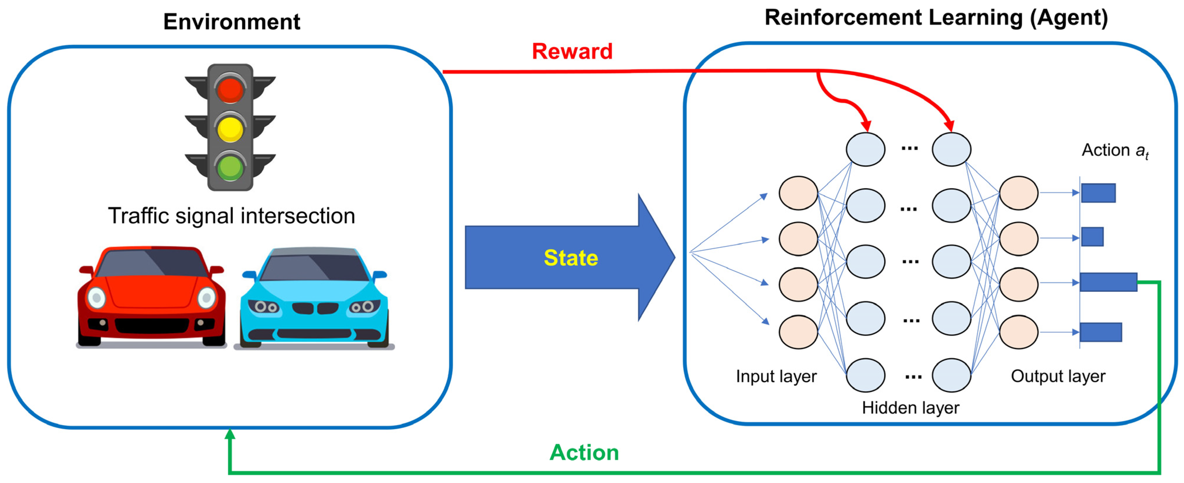
The RL-based traffic signal control model operates on three main components: the agent, the environment, and the elements of state, action, and reward (see
Figure 1). In this model, the agent represents the traffic signal control system, which determines the duration of green, red, and yellow lights based on the current traffic conditions at the intersection. The environment encompasses the surrounding traffic conditions that influence the agent, including the number of vehicles, traffic flow speed, and congestion levels. The state describes explicitly the traffic situation at a given moment, for example, the number of vehicles waiting in different lanes and the remaining time for each traffic light cycle. The action refers to the decision made by the agent, such as adjusting the traffic light duration for each lane, with options like extending the green light for lanes with heavier traffic. The reward reflects the performance of the action taken by the agent and is calculated based on factors, such as vehicle wait time and the level of traffic congestion.
Q-Deep Learning system is a combination of Q-learning and DNNs designed to map the states in the system into the Q-value, representing values related to behavior from changes in external environmental conditions. For traffic light controller problems, Q-learning can be expressed by the following formula:
where
is the Q-value, which is updated in a decreasing manner depending on the learning rate
and the action value at state
. Meanwhile,
is the reward value estimated after performing the action state step
. Furthermore, the
is represented the Q-value in the next state, and
is the next state after finishing the current state
. In addition,
indicates that the action has the highest value among the potential actions at the selected state
. Another parameter,
, is the discount factor indicating that the future reward is less important than the present, and its distribution value ranges from 0 to 1. Following the application of Q-learning in traffic light controller research, Equation (1) can be simplified as follows:
where
is the Q-value corresponding to action
at state
. There is a rule that the updated Q-value of the current action is performed in state
with immediate reward as well as the decreasing Q-values of the actions in the future. Therefore,
is represented by the Q-value of the action in the future, holding the largest reward value after performing state
. Similarly,
and
hold the maximum reward value in the next states
. This is how the agent will choose an action based not only on the current reward but also on the expected future discounted rewards. This rule can be simplified as follows:
where y is a random value indicating the last time step before the end of the episode. Also, since there are no more feasible actions in state
, the value of
is 0. To solve Equation (3), specialized computational software, such as MATLAB lastest version or ealier, can be used; however, it is necessary to limit the number of elements of the chain to easily control the complexity of the calculation. For practical problems, DNNs is used to solve Equation (3) more effectively through the machine learning training process.
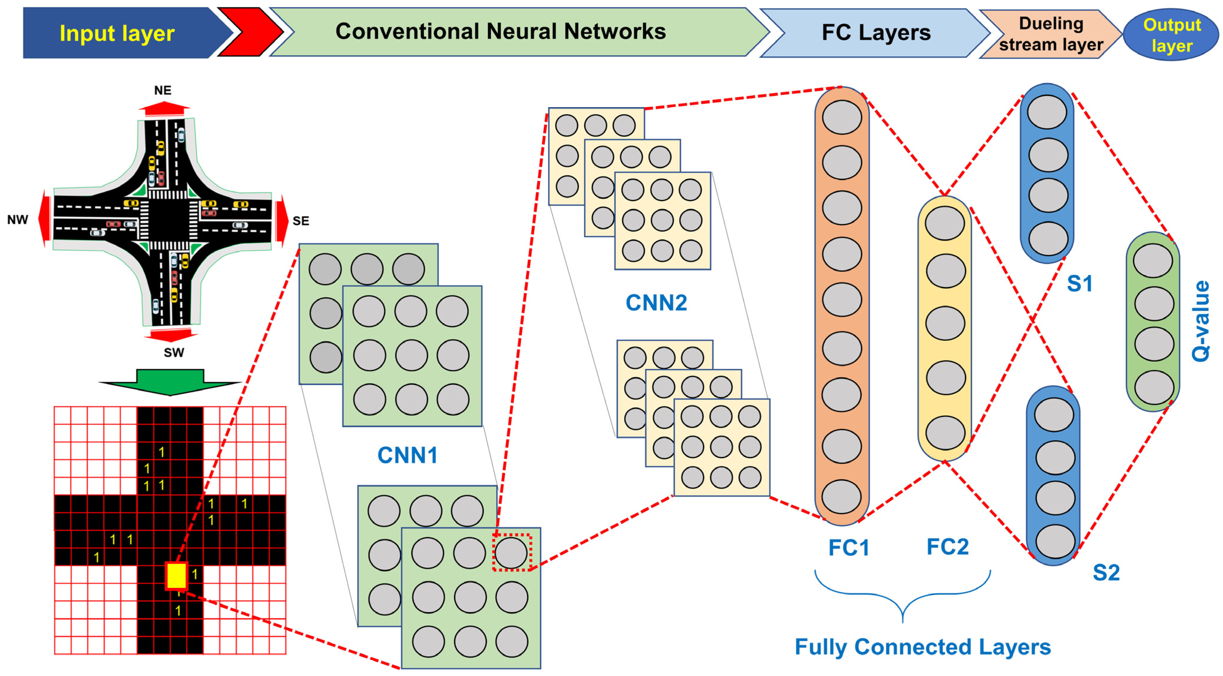
The 3DQN algorithm is an advanced reinforcement learning method that builds upon the traditional DQN by addressing key limitations, such as overestimation bias and improved value decomposition. It begins by initializing two neural networks: the dueling Q-network
, which estimates the action-value function with the random weights
and the target Q-network
initialized with weights
, which helps stabilize the learning process. The networks are designed with separate streams for estimating the state-value function
and advantage function
. As a result, the Q-value can be computed as:
Following Equation (4), this decomposition allows the agent to efficiently learn both the value of being in a state and the advantage of each action.
In addition, a relay memory buffer
, which stores
last transitions, is also initialized and populated with
random transitions
, which store the agent’s past experiences. At the beginning of each episode, environment state
is observed. While the episode is ongoing and the terminal state is not reached, the agent must select action
. The action selection follows two parameters with probability
and random action
. With probability
, the action that maximizes the Q-value is expressed as:
This policy ensures a balance between exploration and exploitation as the agent learns optimal actions. Upon selecting an action, the agent executes it in the environment and observes both the immediate reward
and the next state
. The transition
is stored in relay memory
. In order to update the network, a back-propagation is adapted with a batch
of
transitions
randomly sampled from
. For each sampled transition, temporal difference (TD) error
is computed to update the Q-values of both online and target networks based on the forward propagation process. Therefore, it can be estimated as:
where
is the discount factor, and
is the target network’s Q-value for the next state-action pair.
Following TD error
, the Huber loss function is minimized to update the online Q-network, and it can be computed as:
The Huber loss is minimized using the Adam optimizer, which adjusts weight
based on gradient
. Therefore, the weight matrix of online network Q can be updated as:
where
is the learning rate, which controls the epoch in training process.
In addition, the target Q-network is updated using a Polyak averaging update
where
is a small value which allows the target network to slowly monitor the online Q-network.
Finally, the exploration rate
is decayed exponentially after each time step to progressively shift the focus from exploration to exploitation as the agent learns the optimal policy:
where
is a decay factor. This ensures that the agent explores sufficiently in the early stages of training while increasingly exploiting learned knowledge as training progresses. This iterative process of action selection, experience replay, Q-network updates, and exploration–exploitation balance is repeated for each episode, resulting in an agent that learns an optimal policy over time.
4. Evaluation of 3DQN
This study applied the 3DQN model to optimize traffic signal control at intersections and compare its performance with a fixed three-phase signal control method.
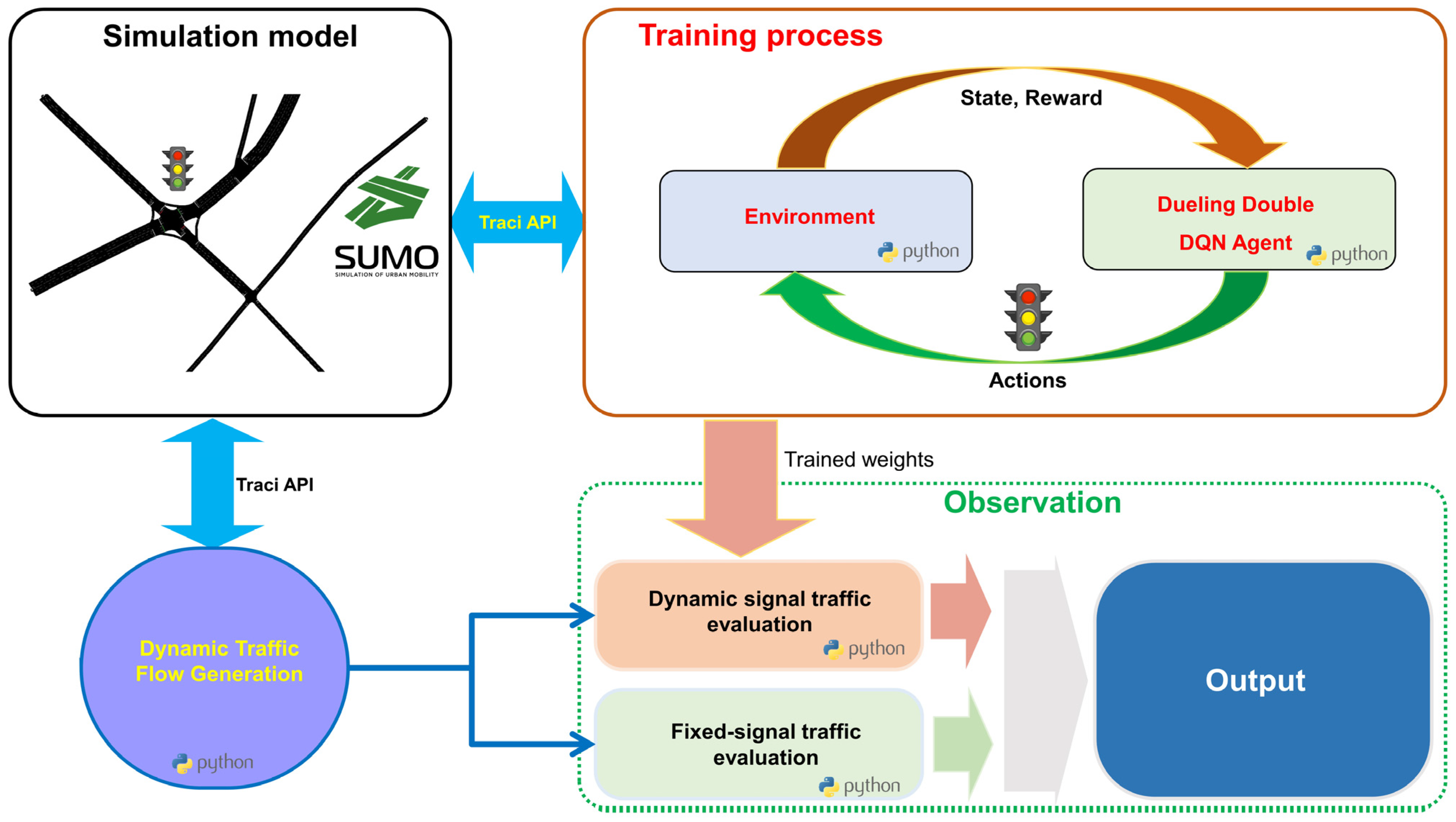
Figure 8 illustrates this optimization process through a flowchart of the 3DQN agent. Before training, a simulation model was constructed using simulation in SUMO software version 1.11 [
34], with the geometric design parameters of the intersection configured according to design standards. Traffic flow within the model was defined based on actual peak-hour traffic flow data.
The Traffic Control Interface (TraCI) API is an application programming interface that enables external scripts to interact with the SUMO simulation model. Through the TraCI API, SUMO is integrated with Python 3.6, enabling real-time control within the simulated environment [
12,
28,
29,
35]. This intersection simulation model is subsequently used as the environment for training the 3DQN agent. SUMO provides the agent with environmental states and rewards, guiding the agent in learning an optimal control policy. The agent returns actions in phase timing for the traffic signals, which are then implemented back into the simulation. This interactive loop facilitates continuous learning, enabling the agent to adapt its strategy based on real-time feedback from the environment.
A dynamic traffic flow generation module, also connected to SUMO, further enhances the simulation flexibility by varying traffic flow randomly from 50% to 150% of the reference flow. This method provides variability in traffic conditions, ensuring that the 3DQN model can handle unstable traffic scenarios in real-world applications—an essential factor for future applications. In addition, demand-responsive traffic signal control is analyzed. For simplicity, a connected vehicle (CV) penetration rate factor is assumed to vary randomly between 0 and 1. This factor is calculated using the binary matrix of CV position P, where 1 indicates the presence of a CV and 0 indicates its absence. The matrix of CV speed V, normalized to the speed limits of the approaches, is also used. The penetration rate is combined with vehicle speeds to introduce variability into the SUMO simulation. Applying this factor will assist in evaluating the performance of traffic signal control using the 3DQN model. For a more detailed explanation of this factor and reward function of DQN, refer to the study by Ducrocp and Farhi [
28].
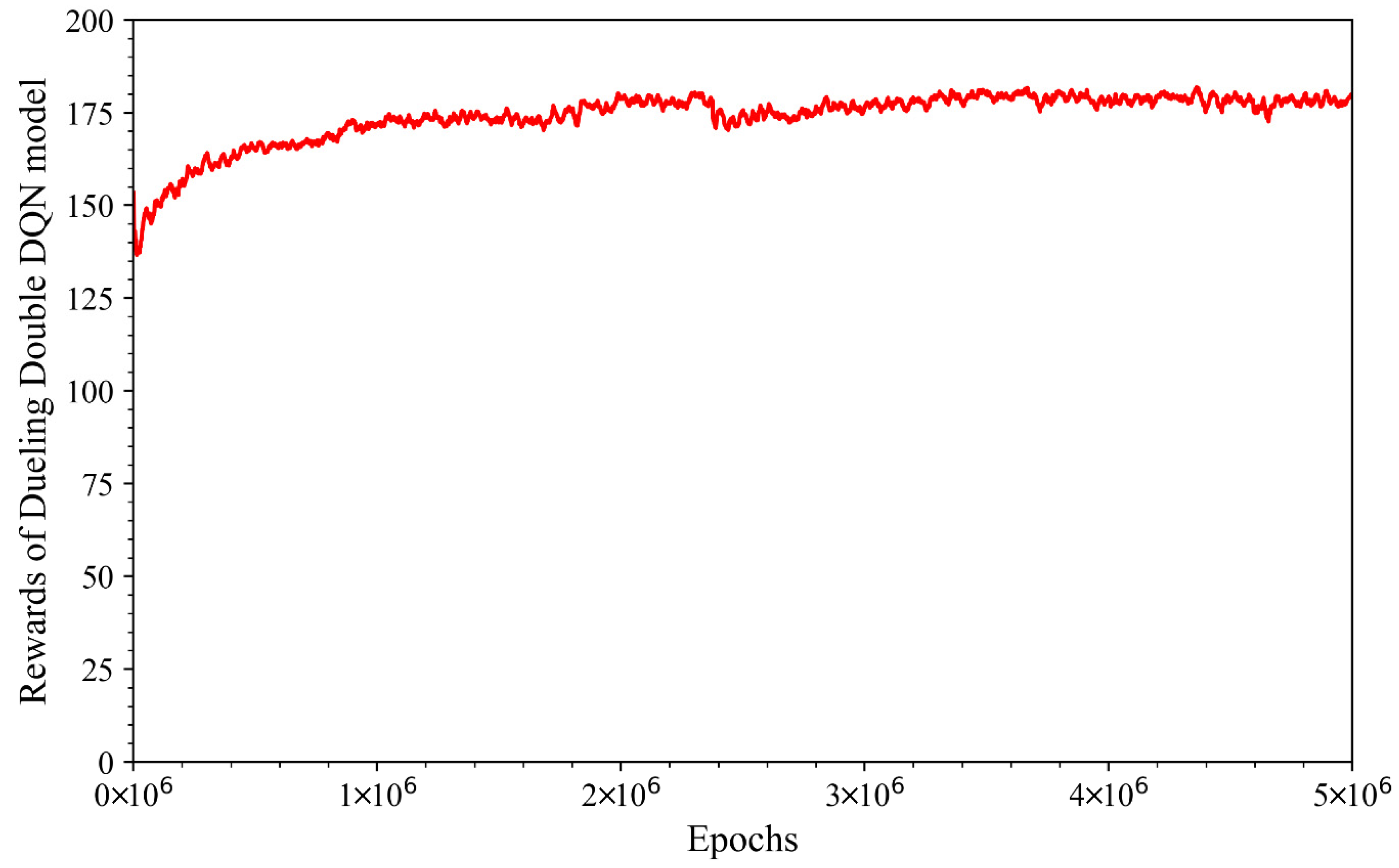
Figure 9 shows the variation in the reward value of the 3DQN model during training, reflecting the model performance improvement across training steps. Initially, the reward value exhibits large fluctuations, possibly because the model has not yet fully learned the system characteristics in an environment with fluctuating traffic flow. However, the reward value begins to gradually increase and stabilize from the 1.5 millionth training step, maintaining stability from the 3 millionth to the 5 millionth training step. The small fluctuations in the curve are a common phenomenon in reinforcement learning, as the model experiments with different strategies before stabilizing and finding the optimal strategy. To evaluate model performance, the weight matrices of the model at the 1 millionth (1M-Step) and 5 millionth (5M-Step) training steps were saved and compared during the model evaluation step to assess the impact of the number of training steps on the learning process and the effectiveness of the 3DQN model.
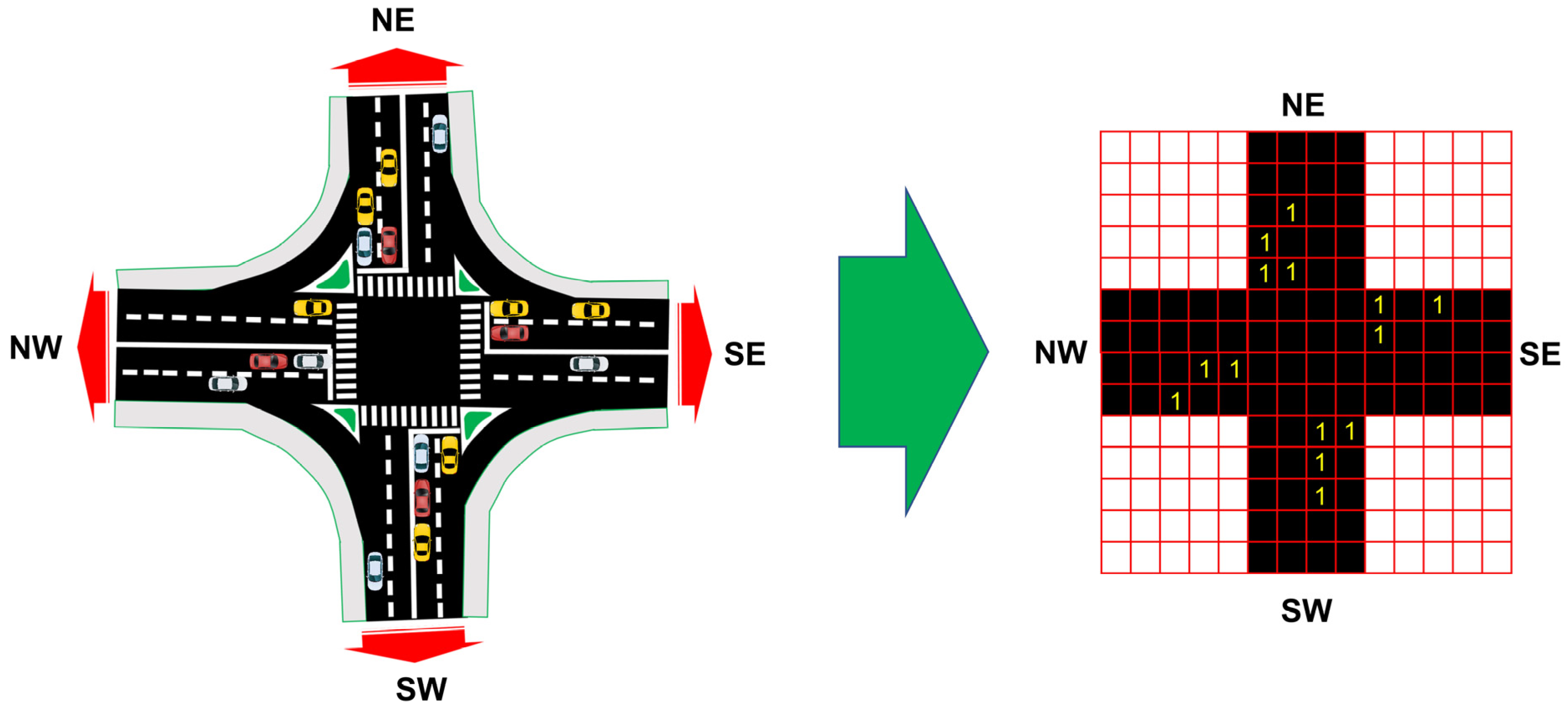
Upon completion of training, the 3DQN model is evaluated by comparing its performance with that of the fixed-signal control method. Two separate evaluation modules are employed, with the 3DQN evaluation module utilizing the trained weight matrix of the agent. In contrast, the fixed-signal control evaluation module simply uses TraCI API to interact with the SUMO simulation model, employing pre-established fixed three-phase signals (
Figure 4). The dynamic traffic flow generation module generates the input traffic flow for both modules, ensuring that both methods are under the same traffic conditions. The results are then compiled in the output block, enabling a detailed comparison of the performance between dynamic and fixed-signal control. These findings offer valuable insights for recommending the practical application of 3DQN to improve traffic efficiency under various conditions.
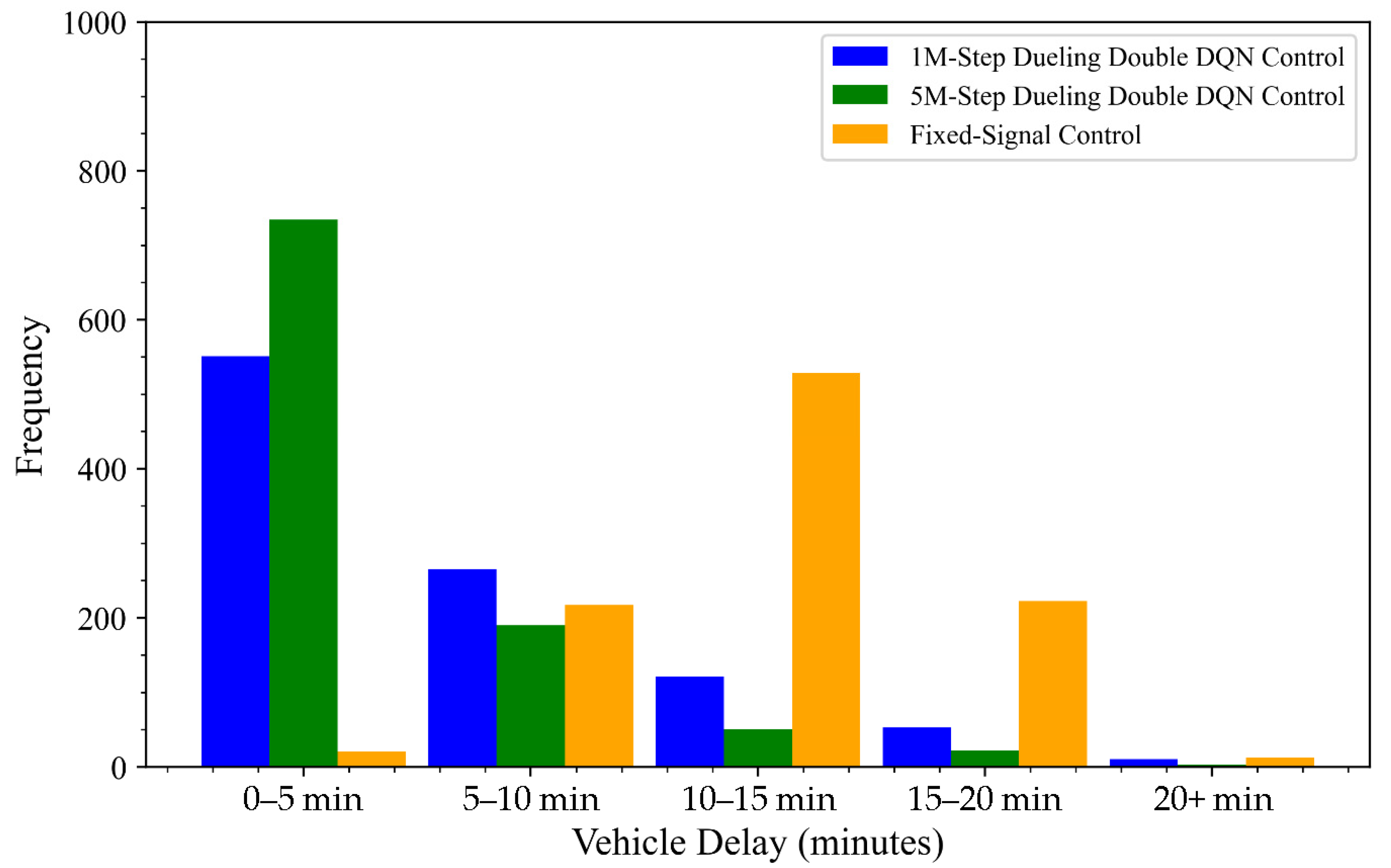
Figure 10 presents the frequency distribution of vehicle delays under two traffic signal control methods—3DQN and fixed-signal control—based on a 1000-h simulation using the SUMO platform. The 3DQN method was tested using two pre-trained models: one trained for 1M-Step and the other for 5M-Step. The x-axis represents vehicle delay intervals (e.g., 0–5 min, 5–10 min), while the y-axis indicates the frequency of each delay interval.
The results clearly differentiate the performance of the two approaches. Both 3DQN models (1M-Step and 5M-Step) significantly reduce the frequency of long waiting times (over 5 min) compared to the fixed-signal control method. This highlights 3DQN’s ability to dynamically adapt to changing traffic conditions, thus improving traffic flow and mitigating congestion. In contrast, while the fixed-signal control method exhibits a higher frequency of short delays (0–5 min), it also shows a substantial rise in delays exceeding 10 min, revealing its limited capacity to respond to variable traffic patterns.
When comparing the two 3DQN models, the 5M-Step model outperforms the 1M-Step model by achieving 750 instances of vehicle delays under 5 min, compared to 550 instances for the 1M-Step model. Furthermore, the 5M-Step model records a significantly lower frequency of delays over 5 min. These findings suggest that the number of training steps has a substantial impact on the model’s performance and stability in real-world conditions. Hence, selecting an appropriate training duration is critical to ensuring that the 3DQN model reaches its full potential and effectively adapts to dynamic traffic environments.
To assess the impact of the CV penetration rate coefficient, vehicle delays were surveyed and analyzed when applying both traffic control methods: 3DQN and fixed-signal control.
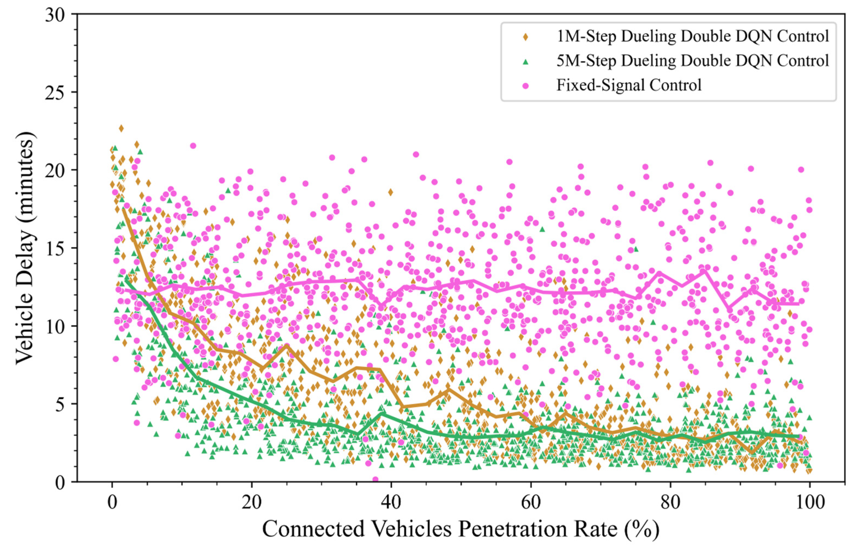
Figure 11 presents a chart showing the distribution of vehicle delay and the CV penetration rate for the two control methods: fixed-signal control and 3DQN control. When applying the fixed-signal control method, vehicle delays are randomly distributed with a wide amplitude, and the average waiting time remains almost unchanged as the CV penetration rate increases. This indicates that the traditional method lacks the ability to connect traffic flow information, leading to inflexibility in adapting to traffic fluctuations. Thus, the vehicle delay remains unchanged as the CV penetration rate increases.
In contrast, the 3DQN control method shows a tighter distribution of vehicle delay, which tends to decrease as the CV penetration rate increases. This demonstrates that the 3DQN model can optimize waiting times more effectively when sufficient traffic flow information, such as vehicle locations and speeds, is available, even if the vehicle-connected penetration rate may not be fully complete. Comparing the 1M-Step and 5M-Step Dueling Double DQN models, the results show that the 5M-Step model is more stable and can reduce the average waiting time to under 5 min when the CV penetration rate reaches 20%, while the 1M-Step DQN model requires a penetration rate of over 40%. It is worth noting that both the 1M-Step and 5M-Step models begin to stabilize and optimize vehicle waiting times to 3–4 min when the CV penetration rate reaches 70% or higher. Therefore, the 5M-Step model proves to be more efficient, requiring only about 20% of the information from traffic flow. In comparison, the 1M-Step model needs 40% of the vehicles in the flow to be connected to the traffic control system. This difference indicates that the number of training steps in the model plays a key role in the system’s flexibility to adapt when full vehicle-connected information is unavailable.
5. 3DQN Performance in Mixed Traffic Patterns
The 5M-Step 3DQN model has demonstrated superior performance in optimizing vehicle delays at intersections. The traffic flow data presented in
Section 4 is based on random traffic simulated over a period of 1000 h, using static traffic values corresponding to peak hours. However, this data does not fully represent the complex fluctuations of real traffic flow, which vary over time and depend on many factors, such as peak hours, weather conditions, or unusual traffic events. To accurately evaluate the impact of MTF on the performance of the 5M-Step 3DQN model, this section presents the process of collecting and processing MTF data, as well as the method for evaluating the model’s performance under real conditions.
MTF data at the signalized intersection is collected through the installed camera system, using the YOLOv8 model [
36,
37] to detect and classify vehicles, combined with the SORT (Simple Online and Real-time Tracking) algorithm [
38] to track and determine the direction of movement of each vehicle type. The classified vehicle types include motorbikes, cars, trucks, and buses. To ensure consistency with the training data of the 5M-Step 3DQN model, the dynamic traffic volume of each vehicle type is converted to the equivalent passenger car unit, a common standardized unit in traffic research. The pre-trained 5M-Step 3DQN model will be integrated with the SUMO to evaluate the performance under dynamic traffic flow conditions, more accurately reflecting real-life traffic scenarios that change over time.
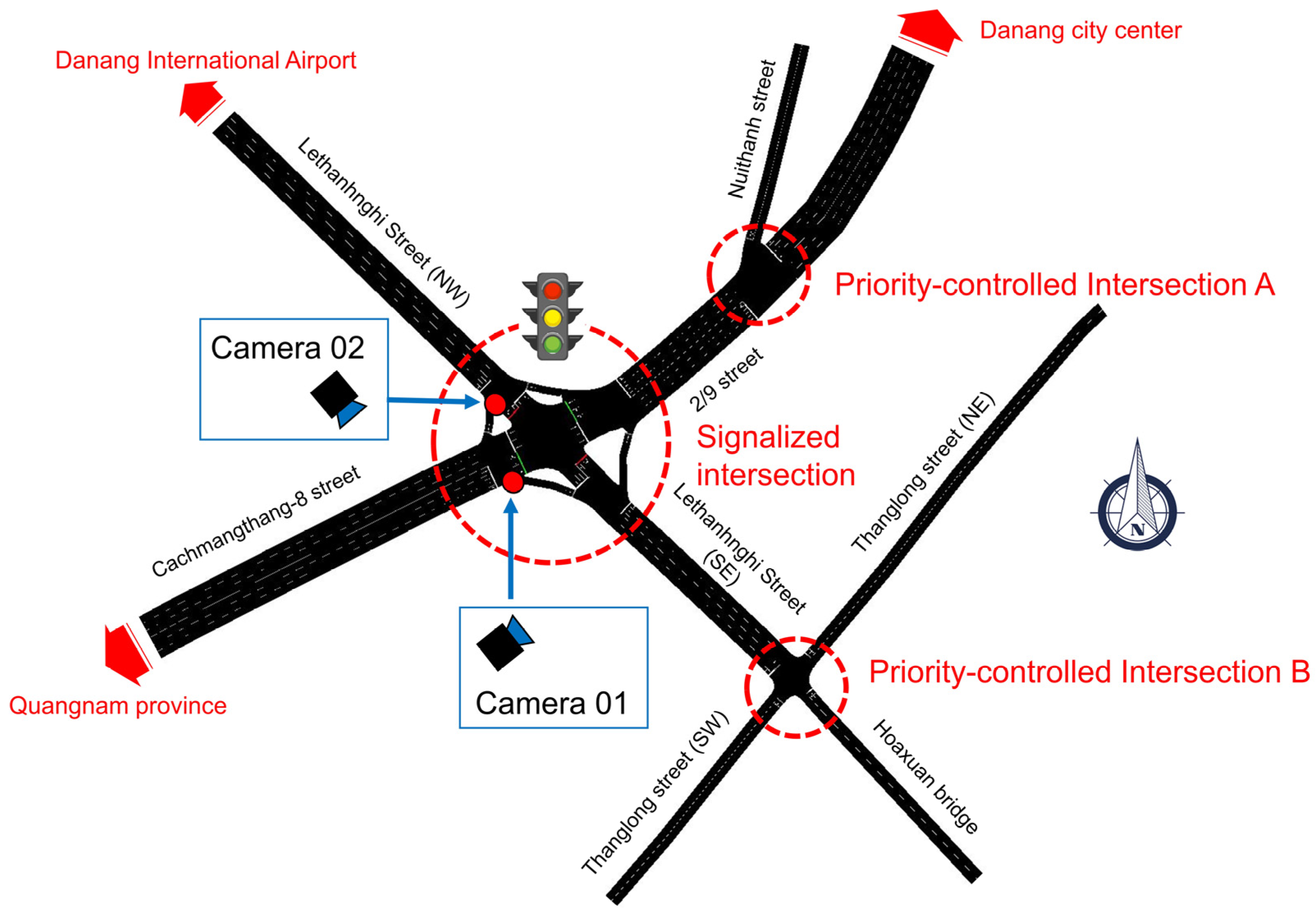
MTF data were collected at the signalized intersection on April 1, 2025 (from 6:00 to 18:00) to evaluate the effectiveness of the 5M-Step 3DQN model. Two cameras were installed at the intersection: Camera 01, recording the direction from Cachmangthang-8 Street to the center of Danang City, and Camera 02, recording the direction from the international airport approach road (Lethanhnghi) to Hoaxuan Bridge.
Figure 3 illustrates in detail the installation locations of the two cameras at the signalized intersection, ensuring coverage of the main traffic flows. However, due to the limitation of the number of cameras, the dynamic traffic flow in directions not directly recorded is estimated based on the traffic ratio of the two main directions recorded by the cameras. This ratio is determined through the analysis of peak hour traffic volume, ensuring the representatives of actual traffic conditions.
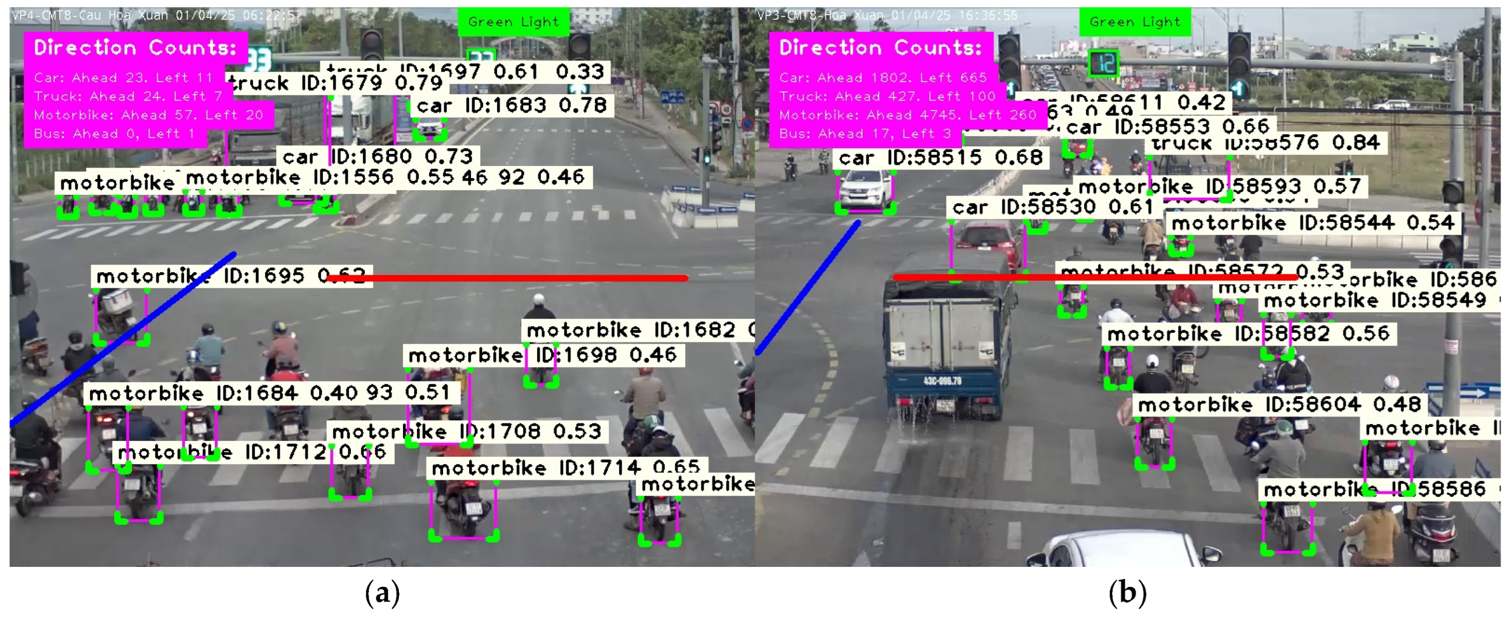
To perform the analysis, a custom-built program was developed based on the pre-trained YOLOv8 model and the SORT library in Python. This program allows for accurate determination of the traffic volume and direction of movement of various types of vehicles, including motorcycles, cars, trucks, and buses. At each camera, two lines are set up to record the traffic volume in two directions: straight and left turn, as illustrated in detail in
Figure 12. In this figure, the red line is used to count the number of vehicles going straight, while the blue line is used to count the number of vehicles turning left. Since the cameras are oriented towards the intersection, an additional algorithm was developed to determine the color of the traffic light to ensure that vehicle counting is only performed when the traffic light is green, allowing vehicles to move in the straight or left turn direction. In addition, each vehicle recognized by the YOLOv8 model is assigned a confidence score, which evaluates the accuracy of the prediction process. This score plays an important role in evaluating the performance of the recognition model. The SORT algorithm is then used to track and determine the direction of each vehicle based on its trajectory. When a vehicle passes the direction line (whether going straight or turning left), the corresponding vehicle type count is recorded and accumulated in real-time. This result provides detailed data on dynamic traffic flow by vehicle type and direction, creating a basis for evaluating the performance of the 5M-Step 3DQN model in optimizing waiting time and traffic management at the intersection.
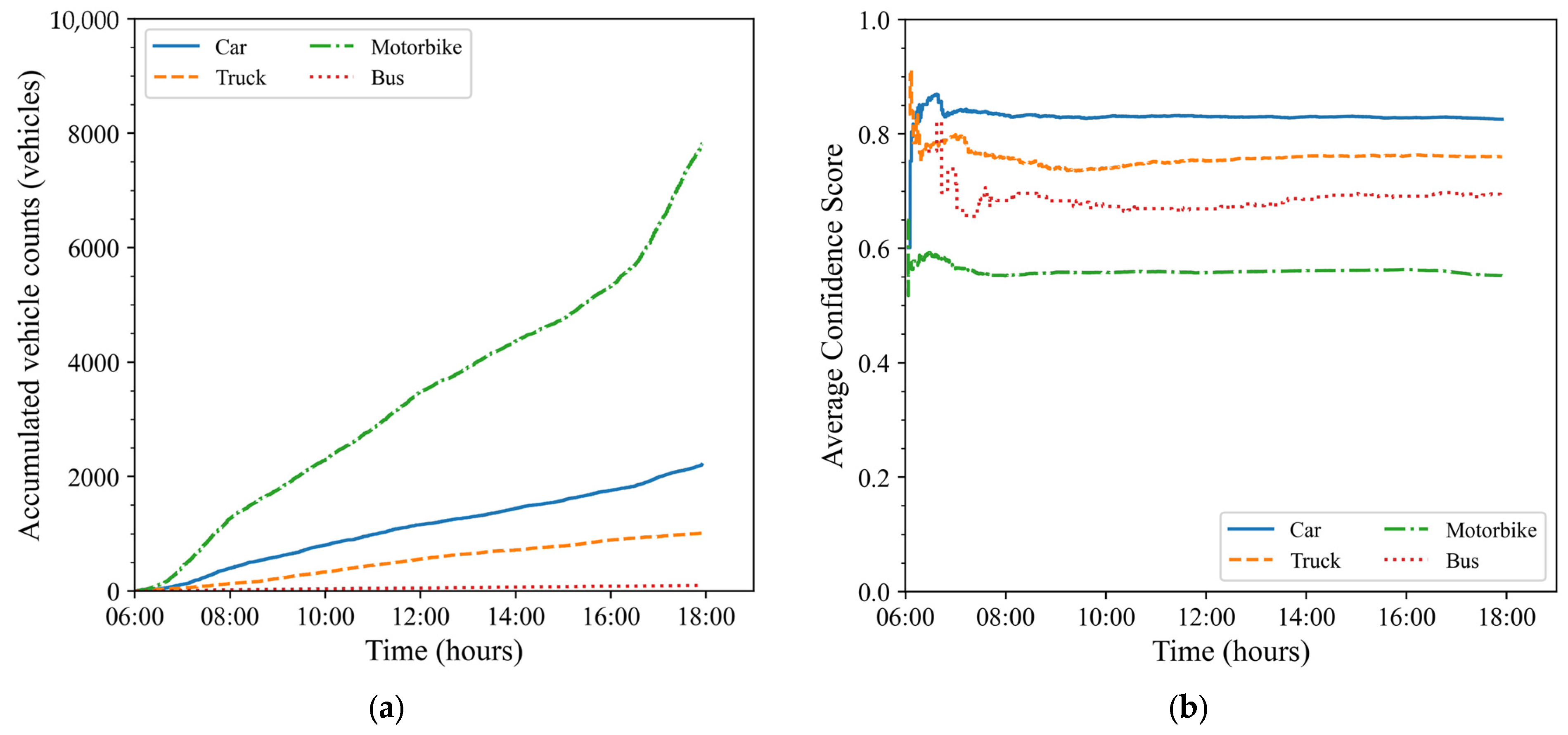
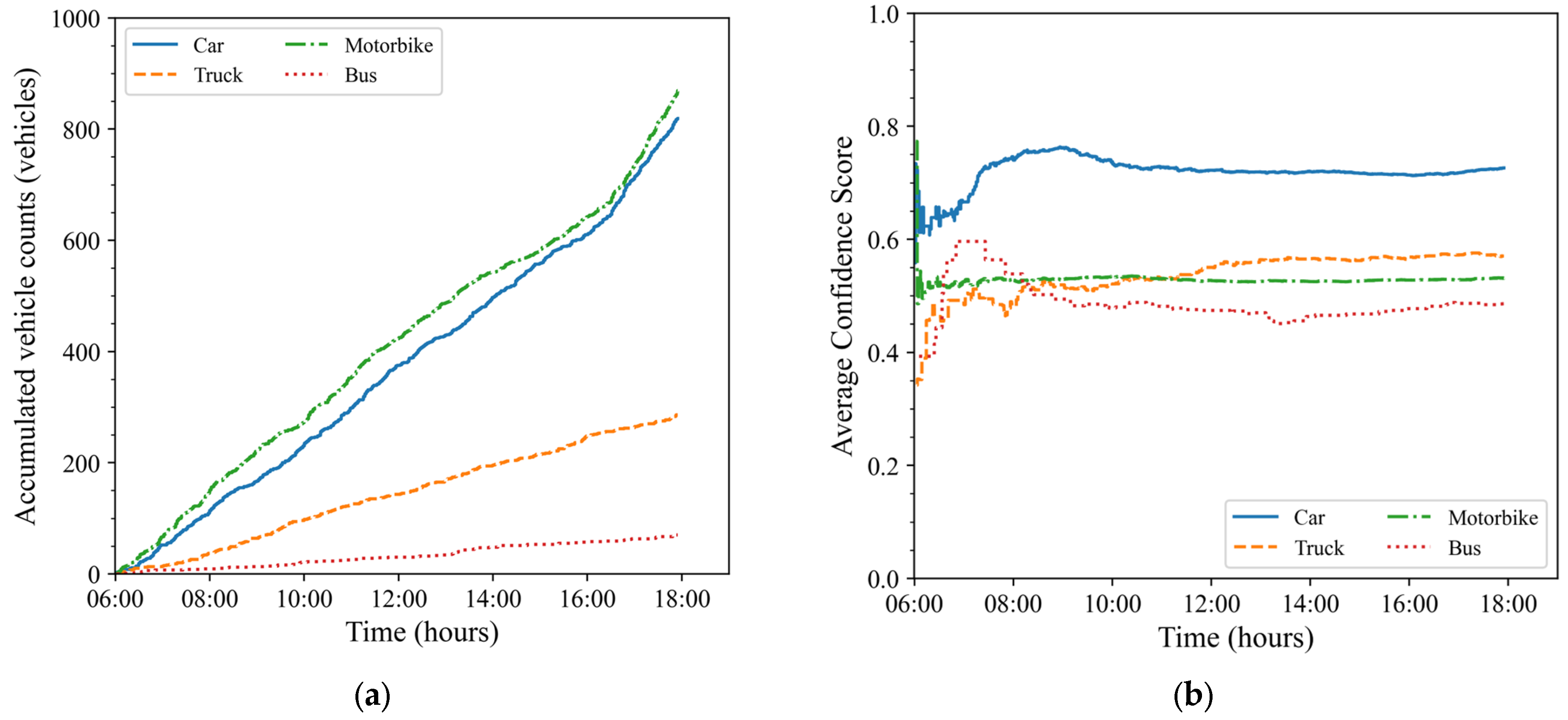
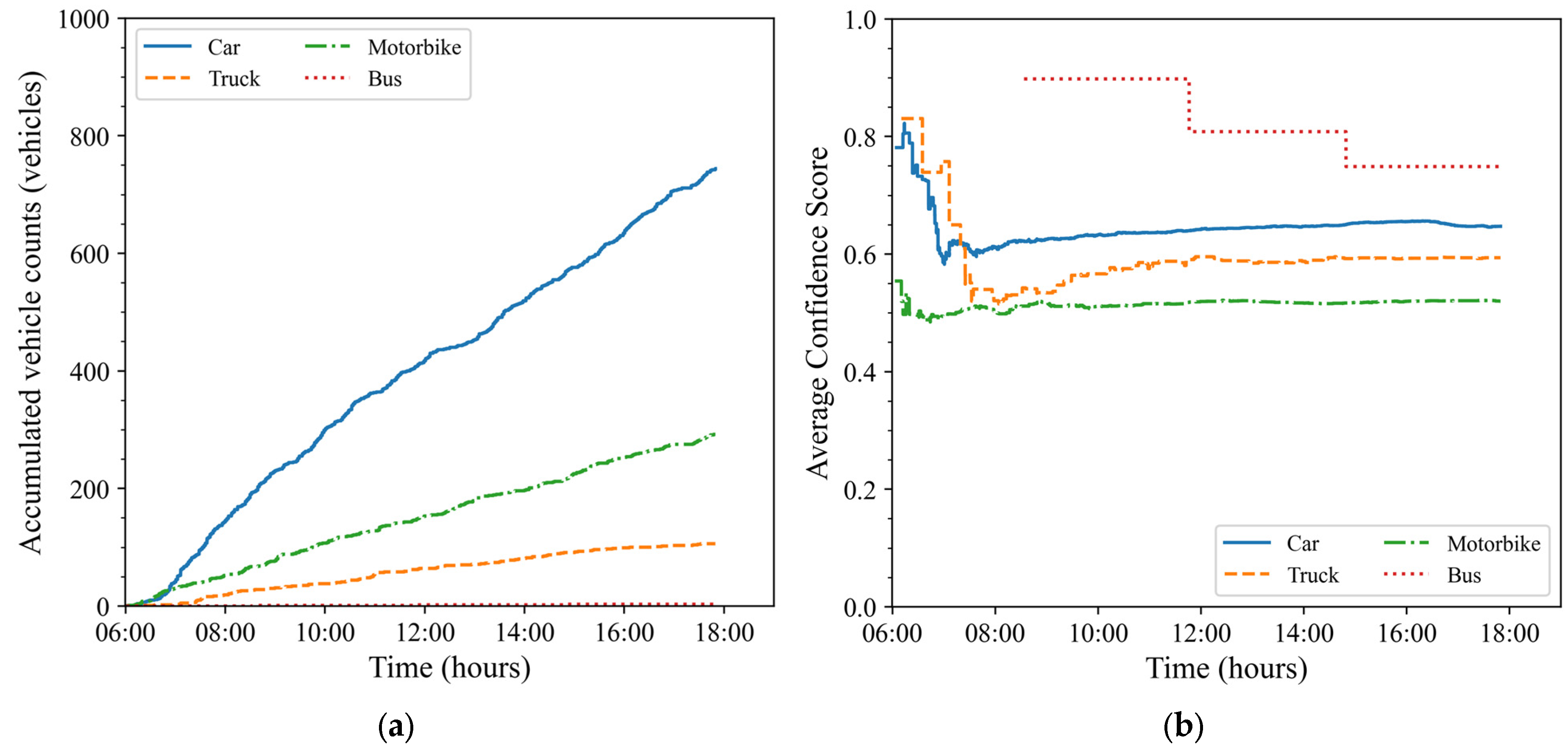
Figure 13 and
Figure 14 show the cumulative traffic volume of vehicle types and the confidence scores of the YOLOv8 model from the image data of Camera 01 in two directions: straight and left turn, respectively. The overall analysis shows that the traffic volume of straight vehicles, as recorded from Camera 01, accounts for the majority compared to the left turn direction. In the straight direction, from Cachmangthang-8 Street to the center of Danang City, motorbikes are the type of vehicle with the highest traffic volume, followed by cars and trucks. Notably, in the left turn direction, from Cachmangthang-8 Street to Lethanhnghi Street towards Danang International Airport, the recorded traffic volumes of motorbikes and cars are similar. Regarding the prediction performance of the YOLOv8 model, the average confidence score in the first stage shows fluctuations, possibly due to the limited number of recognized vehicles. However, when the traffic volume increases, the model shows stability with the confidence score remaining high and fluctuating little over time. Specifically, in the straight direction (
Figure 13), large vehicles, such as cars, trucks, and buses, have high confidence scores, ranging from 0.75 to 0.9, while motorcycles have lower confidence scores, ranging from 0.55 to 0.6. In the left turn direction (
Figure 14), the confidence score of motorcycles is similar to that of trucks and buses but still lower than that of cars. The reason may come from the diversity in color, size, and purpose of use of motorcycles, as well as factors, such as the driver’s clothing or the goods carried, making it difficult for the YOLOv8 model to accurately recognize them.
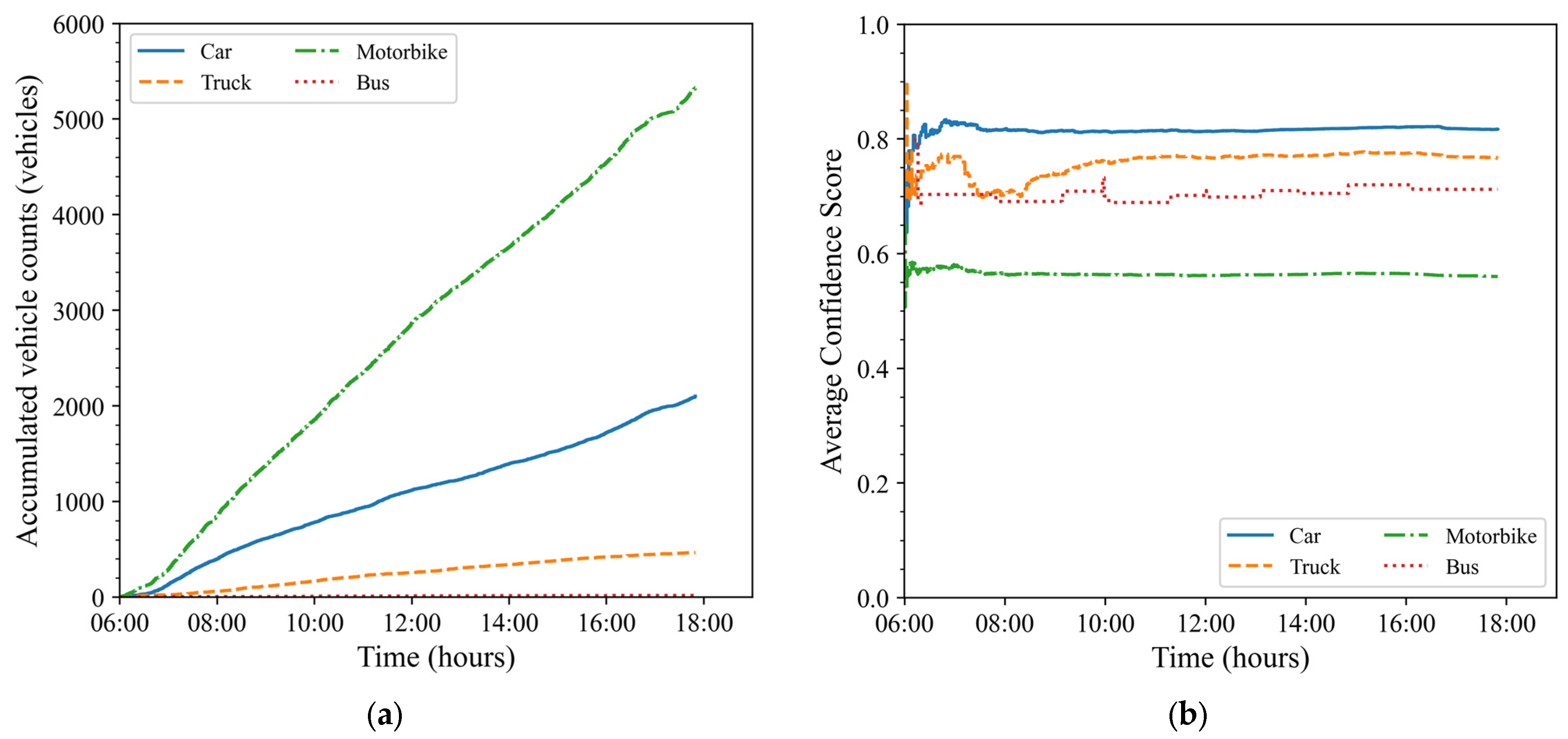
Figure 15 and
Figure 16 show the cumulative traffic volume of vehicle types and the predicted confidence score of the YOLOv8 model from the image data of Camera 02 in two directions: straight and left turn. The overall analysis shows that the traffic volume of vehicles going straight, as recorded by Camera 02, accounts for the majority compared to the left turn direction. Specifically, in the straight direction from Lethanhnghi Street to Hoaxuan urban area (via Hoaxuan Bridge), motorbikes are the type of vehicle with the highest traffic volume, followed by cars and trucks. Notably, in the left turn direction from Lethanhnghi Street to 2/9 Street towards the center of Danang City, cars account for the majority of traffic volume, far exceeding other types of vehicles. Regarding the prediction performance of the YOLOv8 model, the average confidence score shows a similar fluctuation to the data from Camera 01, especially in the early stages when traffic volume is still low. According to the data from
Figure 13,
Figure 14,
Figure 15 and
Figure 16, the average confidence score of all vehicle types at both Camera 01 and Camera 02 locations ranges from 0.5 to 0.9. This confidence score is considered acceptable for use in the performance analysis of the 5M-Step 3DQN model when integrated with the SUMO traffic simulation software.
Following the MTF database, which is collected cumulatively at two surveillance camera locations, the hourly average traffic volume is calculated to optimize data input into the SUMO model. These data are combined with the pre-trained datasets of 5M-Step 3DQN to improve the accuracy of traffic flow analysis and prediction. To ensure consistency and comparability between vehicle types, the hourly average traffic volume of each vehicle type is converted to the equivalent passenger car unit. The conversion factor applied to each vehicle type is as follows: motorbike is 0.3, car is 1.0, bus is 2, and truck is 2.5. These factors reflect the impact of each vehicle type on traffic flow, based on their size, weight, and operating characteristics.
The results of the average hourly traffic volume analysis for the travel directions recorded at Cameras 01 and 02 are illustrated in detail in
Figure 17 and
Figure 18, respectively. Specifically,
Figure 17 presents data on the traffic volume of vehicle types and the corresponding converted car traffic volume at Camera 01. The data show significant fluctuations during peak hours, especially from 7:00 to 9:00 and from 16:00 to 18:00 for the straight travel direction. During this period, traffic volume increases sharply, reflecting the high vehicle density resulting from increased travel demand during morning and evening rush hours. For the left turn direction, traffic volume recorded two distinct peaks around 10:00 and 14:00, and there was a sudden increase during peak hours from 16:00 to 18:00. This variation shows different traffic behavior between travel directions, which may be related to factors such as work or study routes or socioeconomic activities in the area. Similarly,
Figure 18 shows the average traffic volume data of converted vehicles and cars at Camera location 02.
Using the 12-h average traffic data from two camera locations, traffic volumes in other directions at the intersection were estimated as percentages based on the main recorded flows. This dynamic data was input into the SUMO simulation, using the pre-trained 5M-Step 3DQN model to evaluate its performance under real traffic conditions. A fixed-signal control model was also simulated for comparison. For simplicity, both models assumed a CV penetration rate of 1.0.
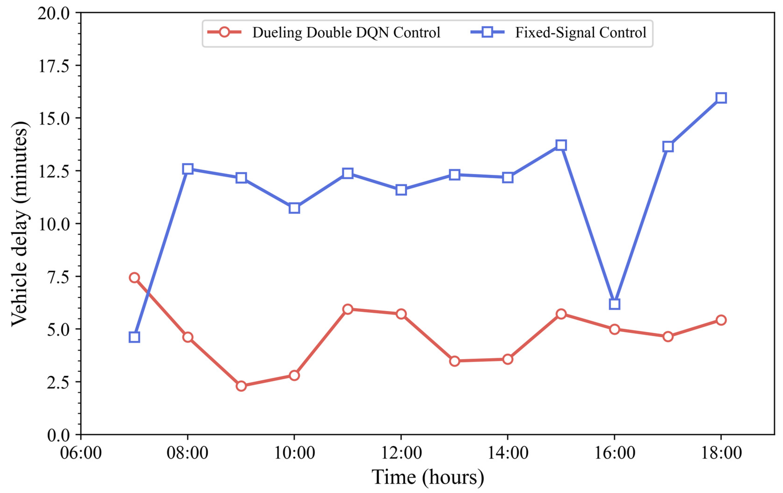
Figure 19 compares vehicle delays between the two models. The graph illustrates a comparative analysis of average vehicle delay (in minutes) across various hours of the day between two traffic control methods: 3DQN control (in red with circles) and fixed-signal control (in blue with squares). The X-axis represents different time intervals throughout the day (though exact times are not labeled, the intervals are consistent). The Y-axis shows the average vehicle delay in minutes.
The 3DQN control consistently achieves lower vehicle delay than the fixed-signal control at all time intervals. The fixed-signal control shows greater variability and higher peaks, with delays exceeding 12 min during some intervals. In contrast, the 3DQN-based model keeps delays mostly under 6 min, with relatively stable performance. The performance gap is especially pronounced during periods of peak congestion (e.g., rightmost section of the graph), where the fixed control experiences a sharp increase, while the 3DQN model maintains low delay.
At 06:00, the 3DQN model showed delays of 7–8 min, while fixed-signal control delays were under 5 min. This matched the rising morning traffic recorded by Camera 02. As traffic increased further, the 3DQN delay dropped to 2 min by 10:00, while the fixed-signal control delay spiked to 12.5 min, remaining high until 10:00. From 10:00 to 12:00, the 3DQN delay increased to 5 min and peaked again at 6 min between 14:00 and 15:00, likely due to midday traffic. The fixed-signal delay also rose, reaching 14 min. After 15:00, both models experienced a decline; however, 3DQN remained stable for approximately 5 min, while the fixed-signal control dropped to 6 min. During the evening peak (16:00–18:00), 3DQN delays remained steady at 4–5 min. In contrast, fixed-signal control delays increased sharply to over 15 min, consistent with the high traffic recorded by both cameras.
Overall, the 3DQN model consistently handled changing traffic better, keeping delays lower and more stable throughout the day, especially during peak periods. Its performance reflects better adaptability to fluctuating traffic flows compared to the Fixed-signal control method.
The findings of this study are consistent with previous research [
12,
26,
27,
28,
29], which demonstrated the potential and significant benefits of RL in improving traffic signal control under dynamic traffic conditions. A novel contribution of this study is the investigation of the effects of dynamic traffic flows on the performance of 3DQN, an aspect that has not been thoroughly addressed in prior studies. The input traffic data for the SUMO-based 3DQN model were collected from realistic camera footage using the YOLOv8 and SORT models for vehicle detection and tracking. As a result, the 3DQN model applied to a signalized intersection in Danang City, effectively reduced vehicle delays, particularly for longer waiting times, by dynamically adapting traffic signal control to real-time traffic flow.
However, the study has several limitations. The computational cost and training time required for the 3DQN model would be a significant hurdle when scaling the approach to a larger traffic network. In addition, the collected dynamic traffic data are limited, as it relies solely on data from two installed cameras, requiring assumptions about traffic flows in other directions. To overcome this issue, cameras covering all directions at signalized intersections need to be installed to provide comprehensive and accurate data, enabling the 3DQN model to make timely decisions and reduce vehicle delays during peak hours. For future research, exploring hierarchical RL or multi-agent reinforcement learning models could help overcome these challenges and improve coordination across multiple intersections. Furthermore, integrating real-time traffic data from connected vehicles and sensor networks could enhance the model’s adaptability and efficiency in real-world applications. Future studies should also prioritize balancing model complexity with computational efficiency to facilitate the practical implementation of RL-based traffic signal control systems in urban environments.
