Article

Learnable Petri Net Neural Network Using Max-Plus Algebra

by
Mohammed Sharafath Abdul Hameed
,
Sofiene Lassoued
* and
Andreas Schwung
Department of Automation Technology and Learning Systems, South Westphalia University of Applied Sciences, 59494 Soest, Germany
*
Author to whom correspondence should be addressed.
Mach. Learn. Knowl. Extr. 2025, 7(3), 100; https://doi.org/10.3390/make7030100
Submission received: 29 July 2025 / Revised: 9 September 2025 / Accepted: 11 September 2025 / Published: 13 September 2025

Abstract

Interpretable decision-making algorithms are important when used in the context of production optimization. While concepts like Petri nets are inherently interpretable, they are not straightforwardly learnable. This paper presents a novel approach to transform the Petri net model into a learnable entity. This is accomplished by establishing a relationship between the Petri net description in the event domain, its representation in the max-plus algebra, and a one-layer perceptron neural network. This allows us to apply standard supervised learning methods adapted to the max-plus domain to infer the parameters of the Petri net. To this end, the feed-forward and back-propagation paths are modified to accommodate the differing mathematical operations in the context of max-plus algebra. We apply our approach to a multi-robot handling system with potentially varying processing and operation times. The results show that essential timing parameters can be inferred from data with high precision.

1. Introduction

Petri nets are a versatile tool and have been used for decades to model discrete event systems, including manufacturing processes [1], traffic flows [2], or logistics [3]. Various extensions of Petri nets exist, namely timed Petri nets to incorporate the system’s timing [4], coloured Petri nets to integrate various entities within a framework [5], and continuous and hybrid Petri nets extending Petri nets to continuous variables.
However, as Petri nets are essentially a tool for system simulation, they generally lack an easy-to-handle mathematical description, mainly due to the non-linearities caused by the firing of transitions. However, for the important subgroup of timed event graphs, a mathematical representation using tropical geometry, also known as max-plus algebra, exists [6]. The tropical algebra allows for a concise mathematical model of the system behaviour in two different representations, namely the dater and counter representation [7].
Furthermore, while Petri nets have been widely used, they come with the limitation that systems have to be tediously modelled, resulting in a long and expensive modelling process, while dynamic changes to the modelled systems are difficult to account for. Specifically, parameters of Petri nets, e.g., processing and transfer times in timed Petri nets, are typically assumed to be known and constant [7]. This appears to be a considerable limitation, particularly when considering that huge amounts of data are collected and readily available to improve the modeling capability of Petri nets and to adjust the model if the underlying system dynamics change over time.
Unfortunately, approaches to add learning capabilities within Petri nets are mostly lacking. At the same time, the recent tremendous advancements in neural networks and their learning capabilities raise the question of whether these techniques can be applied to the training of Petri nets as well.
In addition, in modern production systems, processing and operation times are often uncertain or time-varying due to disturbances, machine conditions, and dynamic scheduling requirements. This makes it impractical to fix Petri net timing parameters a priori. Our approach adapts these parameters directly from data while preserving the interpretability of the Petri net formalism, thereby supporting deployment in realistic production environments. Furthermore, since Petri nets structurally mirror the actual production system, the learned model can be combined with existing simulation and optimization methods. One possible extension is integration with iterative solvers such as reinforcement learning, where Petri nets can serve as a natural simulation environment.
In this paper, we aim to bridge this gap by formally establishing a connection between certain types of Petri nets, their representation in tropical algebra by means of the dater and counter representation, and certain types of neural networks. This connection enables the representation of Petri nets by an equivalent neural network, paving the way for the use of established learning algorithms from the AI community. At the same time, we can use the equivalence to interpret the resulting neural network as a Petri net, which is highly interpretable. Having an interpretable neural network allows humans to supervise, understand, and evaluate the neural network’s decisions. Hence, while neural networks are a learnable black box system, Petri nets are a graphical, mathematical modelling tool that provides an interpretable representation of the discrete event system.
To this end, we introduce a learnable Petri net that can be used by downstream optimization algorithms like heuristic search and reinforcement learning algorithms to solve problems like job shop scheduling. We show that the state space description in the event domain of a Petri net is equivalent to a one-layer perceptron described in the max-plus algebra domain, followed by a hard-max unit. Establishing this allows the Petri net to be learned using supervised learning by a forward-propagation and back-propagation model adapted to the max-plus algebra domain. The main contributions of this paper are as follows:
  • We formally establish a connection between Petri nets, their representations via max-plus-algebra, and specifically designed neural network architectures.
  • We propose a learnable representation of a Petri net in the max-plus domain, allowing us to derive its parameters from available process data.
  • We propose forward- and backward-propagation algorithms for the architecture, thereby enabling learnable Petri nets. Particularly, we propose a parameter-sharing approach between the date and counter representations, allowing us to learn both representations at once.
  • We apply the approach to an application example from production flow shop modelling to illustrate the feasibility of the approach.
The paper is organized as follows: Related work is presented in Section 2. Section 3 provides the theoretical background of the concepts used throughout the paper. Section 3.5 establishes the theoretical connection between Petri nets and neural networks, while Section 4 presents the learning algorithms. Section 5 and Section 7 conclude the paper with empirical results and discussion.

2. Related Work

In this section, we discuss the related work on Petri nets, their relation to tropical geometry and neural networks, and applications with a focus on production systems.

2.1. Petri Net

The Petri net has been formulated as a low-level network describing the relation between events and states. It has continuously improved over the last few decades to accommodate the increasing complexity requirements in DES modelling [8]. Notable extensions include incorporating processing time in timed Petri nets (TPNs) [4] as well as environmental variability like in stochastic Petri nets (SPNs) and extended stochastic Petri nets (ESPNs) [9]. Further, the possibility to carry different information or instances in the tokens, as in coloured Petri nets (CPNs) [5] has been incorporated. One or more extensions of Petri nets can also be consolidated together to improve modelling capacity, like the extended stochastic coloured Petri nets (ECSPNs) [10]. In fact, ref. [10] developed a Petri net with unique advantages in simulating production systems in Industry 4.0 systems, like high variability, flexibility, communication, self-control, and self-organization. While Petri nets are an interpretable modelling tool, they are not designed to be learnable nor adaptive. In this work, we draw connections between specific Petri nets and neural networks to make Petri nets learnable using standard machine learning algorithms while simultaneously increasing the interpretability of such neural networks.

2.2. Max-Plus Algebra and Neural Networks

We aim to establish a missing link that combines the interpretability of Petri nets with the learning capacity of neural networks while modelling complex processes. We use max-plus algebra [6] to bridge the gap between learning capability and interpretability. Max-plus algebra has been extensively used to describe discrete event systems (DESs) in the context of production planning [7].
The combination of max-plus algebra and neural networks has been investigated in previous work. Initially introduced by [11], the morphological perceptron (MNN) with competitive learning was proposed by [12], showing the utility of MNN in classification tasks. Ref. [13] further examines the properties of morphological classifiers, such as the effect of incorporating morphological perceptrons in layers of neural networks.
Max-plus algebra was also employed to reduce the size of the neural network without sacrificing accuracy [14]. Unlike previously known structured and unstructured pruning techniques, tropical geometry is employed to approximate a neural network by a simpler one whose Newton polytopes are similar. In practice, this method can be faster than pruning techniques.
Ref. [15] leveraged the Newton polytope technique for tropical polynomials to find upper bounds on linear regions of the neural network with piecewise linear activations, allowing them to analyse the representation power and complexity of learning models. Furthermore, the paper considered neural networks with piecewise activation functions as tropical polynomials, taking into account that rectified linear units (RELU) are tropical polynomials of rank two and Maxout units are a generalization of rank k. Motivated by the fact that a ratio of polynomials has better approximation quality compared to a single polynomial with the same degree, ref. [16] showed that a feed-forward network with rectified linear units is analogous to the family of tropical rational maps.
While the above approaches discuss representation capacity and pruning techniques in neural networks, none of the works address the connection between Petri nets, timed event graphs, and neural networks to derive learnable Petri nets.

2.3. System Identification Using Max-Plus Algebra

Tropical regression, also referred to as Linear regression over the max-plus semiring, is commonly used for forward problems in predicting outcomes. Our focus lies in the inverse problem scenario, i.e., we aim to deduce the system dynamics from observed data.
Ref. [17] recasts the problem of state space identification into an extended linear complementarity problem, which leads to identifying the parameters of the state space from input and output sequences. Moreover, mixed integer programming approaches were implemented to further optimize the efficiency. In the case of stochastic systems, ref. [18] proposed two approaches to infer the dynamical systems model based on an observed noisy orbit for a stochastic max-plus linear dynamical system. The first approach is the gradient-based exact solution, and the second approach is a less computation-intensive approximation method based on the higher-order moments of a random variable. The mentioned paper presents individually designed identification methods, while we focus on the relation between tropical geometry and neural networks to allow for standard learning approaches for neural networks. Further, we provide an integrated approach for date and counter representation identification, offering downstream applications particularly in production systems.

2.4. Neural Networks in Production Scheduling

Recent advances in deep learning (DL) architectures have developed at a rapid pace. Consequently, they are increasingly used in industry for applications like fault diagnosis [19], machine remaining useful life predictions [20], etc. Also, DL is a popular method of choice in production planning and control applications [21], where the use of neural networks in production planning and control is primarily focused on the self-organization of resources and the self-regulation of the production process. In the context of smart planning and scheduling, a large portion of the literature solely relies on supervised learning [22,23]. Other approaches attempted to leverage the power of unsupervised learning to preprocess the data before using supervised learning at bottleneck detection tasks in the production line [24,25]. Other approaches also attempt to harness the synergy of combining reinforcement learning with the supervised or unsupervised approaches for scheduling problems, where the RL excels in the decision-making part [26,27].
Specifically, the idea of an algorithm capable of interacting and directly learning from the production environment to continuously enhance its scheduling capability promises robust and reliable performance. To this end, deep neural networks have been used quite extensively in the context of RL for scheduling problems [28,29]. Further, refs. [30,31,32] propose graph-based RL algorithms where graph neural networks (GNNs) were used to model the interactions in job shop scheduling problems (JSSPs), thereby providing a more interpretable representation. The combination of Petri nets and RL has been introduced in [1], where the Petri net models the product flow in the production environment. However, though providing a very interpretable representation of the production environment, this model is not able to adapt itself to a dynamically changing environment, e.g., dynamically varying processing times. In this paper, we bridge this gap in providing a learnable Petri net representation which, at the same time, has a more interpretable representation than the more generic GNNs.

3. Theoretical Background and Relation Between Petri Nets and NN

In this section, we present the theoretical foundations and key components of our approach. We begin with standard Petri nets, followed by coloured Petri nets, emphasizing their modelling advantages and the need for colour unfolding. This unfolding is crucial for transforming the abstract coloured model into an analyzable form compatible with timed event graphs (TEGs). We then introduce max-plus algebra, which provides a mathematical framework for modelling synchronization and timing in discrete event systems using timers and counters. Finally, we outline the fundamental principles of neural networks, laying the groundwork for transforming TEG state-update equations into a learnable structure via a tropical neural network.

3.1. Petri Nets

Petri nets are formal modelling tools used to describe and analyse the behaviour of dynamic systems exhibiting concurrency, synchronization, and resource sharing. They provide both a graphical and mathematical framework to represent system dynamics, enabling analysis of key behavioural properties such as reachability, liveness, and deadlock freedom [33]. A Petri net is formally defined as a pair ( G , μ 0 ) , where G is a directed bipartite graph composed of places and transitions, and μ 0 denotes the initial marking, which assigns a discrete number of tokens to each place.
Unlike conventional graphs, Petri nets consist of two disjoint node sets: places P , representing conditions or states of the system, and transitions T , representing events or operations that can change the state. Arcs define the input/output relationships between places and transitions, modelling token flow. The state of the system is encoded in the marking μ , where μ ( p ) gives the number of tokens at place p. A transition t T is enabled when all its input places contain the required number of tokens; firing it updates the marking as follows:  
μ ˜ ( p ) = μ ( p ) 1 if p π ( t ) , μ ( p ) + 1 if p σ ( t ) , μ ( p ) otherwise ,
where π ( t ) and σ ( t ) denote the sets of input and output places of transition t, respectively. Petri nets effectively model and abstract the general system behaviour [34] and help identify defects or undesirable behaviour such as deadlocks [35].
In real-world systems, parts that share resources but differ in type often require modelling multiple subnetworks, which can cause the Petri net to grow exponentially with increasing variety. To address this, coloured Petri nets (CPNs) were introduced, extending classical Petri nets by allowing tokens to carry data called “colours.” This enhancement enables compact and expressive models of complex systems with structurally similar yet data-distinguished processes, such as job shop scheduling, where multiple jobs compete for common resources [5,36]. Formally, a coloured Petri net is defined as the tuple:
CPN = ( P , T , A , Σ , C , N , E , G , I ) ,
where
  • P = { p 1 , , p m } : set of places;
  • T = { t 1 , , t n } : set of transitions;
  • A = { a 1 , , a k } : set of arcs;
  • Σ = { c 1 , , c l } : set of colours (data types);
  • C : P T Φ ( Σ ) : colour function assigning a colour set to each place and transition;
  • N : A ( P × T ) ( T × P ) : node connectivity function defining the source and target of each arc;
  • E : A expressions : arc expression function specifying the token expressions for each arc;
  • G : T { 0 , 1 } : guard function assigning Boolean expressions controlling transition enabling;
  • I : P initial markings : initialization function specifying the initial coloured token distribution.
Coloured Petri nets facilitate modelling of complex discrete event systems by integrating data values with control flow, enabling compact representations without losing analytical power. This capability is crucial for practical applications such as manufacturing systems, communication protocols, and workflow management, where multiple entities with differing attributes interact concurrently.
Figure 1 illustrates simple examples of different Petri net variants: (a) a basic Petri net showing places and transitions; (b) a coloured Petri net highlighting token differentiation through colours; and (c) a coloured timed Petri net that extends the model by incorporating timing to control transition firing delays.
In Figure 1a, transition t 1 is enabled since its sole upstream place contains a token. Conversely, transition t 2 remains disabled because one of its input places, p 2 , is empty. Thus, t 1 must fire first to enable t 2 .
In Figure 1b, although place p 2 contains a token, transition t 2 is still disabled because the token’s colour does not match the transition’s required colour. Here, “colour” is a simplified representation; in practice, token attributes can be complex data types—such as tuples, vectors, or structured objects—that must satisfy specific conditions to enable transitions.
Finally, Figure 1c introduces timing constraints: a timed transition that cannot fire until the token residing in the upstream place p 4 has completed its specified sojourn time. In our model, this sojourn time is encoded as an attribute of the token, capturing processing durations, transport delays, or similar temporal factors.

3.2. Petri Net Colour Unfolding

While coloured Petri nets offer a compact and expressive way to model complex systems with data-carrying tokens, their colour-based abstraction can sometimes complicate analysis and simulation. In particular, many classical Petri net tools and theoretical results apply only to standard Petri nets.
To bridge this gap, when the colour sets Σ of a coloured Petri net are finite, the CPN can be unfolded into an equivalent standard Petri net that explicitly distinguishes each colour as a separate place or transition [36]. This unfolding process produces a classical Petri net with a larger, but colour-free structure, thereby preserving the original system’s behaviour while enabling the use of standard Petri net analysis techniques.
The following formal definition captures this unfolding procedure [37]:
N * = ( P * , T * , A * , f * , m 0 * ) ,
where
  • P * = { p ( c ) p P , c C ( p ) } : set of unfolded places, one per colour per original place.
  • T * = { t ( b ) t T , b B ( t ) } : set of unfolded transitions, one per binding per original transition.
  • A * = { ( p ( c ) , t ( b ) ) ( p , t ) A , ( f ( p , t ) [ b ] ) [ c ] > 0 } { ( t ( b ) , p ( c ) ) ( t , p ) A , ( f ( t , p ) [ b ] ) [ c ] > 0 } : set of unfolded arcs.
  • f * : A * N : arc weight function defined as
    f * ( p ( c ) , t ( b ) ) = ( f ( p , t ) [ b ] ) [ c ] , f * ( t ( b ) , p ( c ) ) = ( f ( t , p ) [ b ] ) [ c ] .
  • m 0 * : P * N : initial marking function given by
    m 0 * ( p ( c ) ) = m 0 ( p ) [ c ] .
In the unfolded Petri net, each coloured token residing in a place p of the original coloured Petri net (CPN) is represented as a token in a distinct place p ( c ) , effectively separating tokens by their colours. Similarly, each binding b of variables in a transition t leads to the creation of a specific transition instance t ( b ) in the unfolded net. The arcs are instantiated based on the evaluation of colour- and binding-dependent arc expressions, ensuring that the flow of tokens and their multiplicities are preserved according to the semantics of the original CPN. The initial marking is also unfolded, such that each place p ( c ) in the unfolded net is initialized with the number of tokens of colour c specified in the initial marking m 0 ( p ) of the corresponding place p in the CPN.
Now, the Petri net can be unfolded, which represents the crucial first step in transforming any coloured timed Petri net into a choice-free net. This transformation is necessary before we can effectively model the system using max-plus algebra. In the following section, we will further develop this concept by exploring timed event graphs described using max-plus algebra.

3.3. Timed Event Graphs (TEGs)

By definition, a timed event graph is a subclass of Petri nets where every place has exactly one upstream and one downstream transition [38]. TEGs are especially well-suited to model sequential operations and synchronization phenomena. They are further enriched with timing information associated either with transitions or places. Specifically, the duration assigned to transitions is called the firing time β i , while the duration assigned to places is known as the holding time α i . Since transitions represent discrete events, firing times model the elapsed time between the start and completion of these events; conversely, holding times specify the minimum duration a token must remain in a place before enabling downstream transitions.
In a production context, firing time typically corresponds to machining or processing durations, whereas holding time may represent transport delays between production stations or material preprocessing intervals. Another important timing parameter is the lag time  w i in the initial marking, which indicates the delay before a token initially contributes to enabling the downstream transition. At first glance, this lag time resembles the holding time; indeed, if all tokens enter their respective places at t = 0 , then w i = α i .
TEGs can be effectively modelled using max-plus algebra, which offers two complementary representations known as the counter and dater forms [7]. Although these representations are mathematically connected, they address distinct questions. The counter representation describes how many events have occurred up to a given time, while the dater representation specifies the time of the kth occurrence of an event.

3.4. Max-Plus Algebra and TEGs

In this section, we formally derive both the dater and counter representations for timed event graphs, starting with the foundational concept of max-plus algebra. Also known as the tropical semiring, max-plus algebra is defined on the set R { } and is characterized by two fundamental operations [39]:
a b = max ( a , b ) , a b = a + b ,
where and 0 serve as the identity elements for ⊕ and ⊗, respectively. This algebra provides a natural framework for modelling discrete event systems, as it captures the fundamental timing relationships inherent to such systems. In particular, the ⊕ operation models synchronization constraints by representing that an event can only occur after all prerequisite events have completed, while the ⊗ operation models the additive accumulation of delays, so that the occurrence time of an event corresponds to its start time plus its duration.
We assume that both places and transitions operate under a First-In First-Out (FIFO) policy concerning the token flow. Furthermore, the system is assumed to begin from a compatible initial condition, where the initial firing times satisfy w i α i , ensuring the timing model’s consistency.
The state of the system is described by a vector of daters, denoted x d ( k ) = x 1 d ( k ) , , x | Q | d ( k ) , where each x i d ( k ) represents the epoch when the transition q i fires for the k-th time. External inputs to the system are captured by the input vector u d ( k ) = u 1 d ( k ) , , u | U | d ( k ) , where U denotes the set of input transitions. Each input sequence u j d ( k ) is a non-decreasing sequence marking the epochs at which external actions trigger the corresponding transition q j . These input sequences are also assumed compatible with the initial condition, satisfying u j d ( 1 ) 0 , and both x j d ( k ) and u j d ( k ) take the neutral element ε = for all k 0 .
Under these definitions and assumptions, the behaviour of the timed event graph can be compactly described by the max-plus linear dater equation:
x d ( k + 1 ) = A x d ( k ) B u d ( k + 1 ) ,
where A and B are max-plus matrices that characterize the system’s internal dynamics and its response to external inputs, respectively. This equation encapsulates the timing dependencies and synchronization constraints governing the system and provides a foundation for connecting timed event graphs with learnable neural network models.
Then, the dater equation of a TEG is given by
x d ( k ) = A ( k , k ) x d ( k ) A ( k , k M ) x d ( k M ) B ( k , k ) u d ( k ) B ( k , k M ) u d ( k M ) ν ( k ) , k > 0
where M is the maximum number of tokens in all the places:
M = m a x i = 1 , , | P | μ i .
Further, the | Q | × | Q | state matrix A( k , k ),..., A( k , k M ) is given by
A j l ( k , k m ) = def { i π q ( j ) | π p ( i ) = l , μ i = m } α i ( k ) β l ( k m ) .
The input matrix of dimension | Q | × | U | , and values B( k , k ),...,B( k , k M ) is given by
B i l ( k , k m ) = def { i π q ( j ) | π p ( i ) = l , μ i = m } α i * ( k ) ,
where it can be shown that the firing times of the transition can be dissolved into the holding time and assign β j = e without a loss of generality, given by the equation below [6]:
α i * = α i β π p ( i ) ( k μ i ) .
Equation (7) states that the firing time for a transition consists of the previous place-holding time ( α i ) and the firing times of the transition upstream ( β l ). The | Q | -dimensional vector representing the maximum initial lag times in the upstream of a transition υ i ( k ) ,   k = 1 , , M is   
υ j ( k ) = def { i π q ( j ) | μ i k } ω i ( k ) .
Equation (5) can be formatted into the standard form using an extended state vector as shown below: 
x ˜ d ( k + 1 ) = A ˜ ( k ) x ˜ d ( k ) B ˜ ( k ) u ˜ d ( k ) υ ˜ ( k ) ,
where the extended state and input vectors are defined as
x ˜ d ( k ) = def x d ( k ) x d ( k 1 ) x d ( k + 1 M ) , u ˜ d ( k ) = def u d ( k ) u d ( k 1 ) u d ( k + 2 M )
And the extended system matrices are given by
A ˜ ( k ) = A ¯ d ( k + 1 , k ) A ¯ ( k + 1 , k 1 ) A ¯ ( k + 1 , k + 1 M ) e ε ε ε ε e e ε ε ε ε e ε
B ˜ ( k ) = B ¯ ( k + 1 , k + 1 ) B ¯ ( k + 1 , k ) B ¯ ( k + 1 , k + 2 M ) ε ε ε ε ε ε
Alternatively to the dater representation, the counter representation can be used for modelling. Essentially, under mild conditions, the counter is the dual residual of the dater representation [6]. Hence, both representations share the same parameters. However, for our application domain, parameters in the dater representation appear linearly, making learning much simpler in tropical algebra, while the parameters appear as time shifts in the counter representation. Consequently, learning the dater representation also comes with learning the counter representation indirectly.
At the same time, both representations are meaningful for applications. Taking production scheduling as an example, the data representation provides insights into timing-related information, such as the time it takes to produce a sequence of orders. At the same time, the counter offers insights into the number of goods produced. Consequently, both representations can be used as cost functions for optimization.

3.5. Neural Networks and TEGs

Neural networks are universal approximators, which use multiple layers of neurons and non-linear activation functions to learn and represent complex and non-linear relationships between inputs and outputs. The most common model is the Multi-Layer Perceptron (MLP) [40], where a layer with i = 1 N inputs x i and j = 1 M outputs y j is represented by
y j = f ( b j + i = 1 n w i , j x i )
where f ( · ) denotes the activation function, and w i , j and b j are the weights and bias of the layer’s neurons, respectively. Sigmoid and Rectified Linear Units (ReLU) are among the most common activation functions [41].
In this section, we aim to establish conditions for the equivalence of a timed event graph in the data representation and a suitably defined neural network. Achieving this enables us to develop a learnable timed event graph using approaches from neural network training. Specifically, this allows us to learn the firing timing from available system data, which can be used by various downstream tasks.
Let a timed event graph (TEG) be given in its dater representation by Equation (11). An equivalent representation can be constructed using a recurrent neural network consisting of two single-layer maxout networks, combined via an element-wise max-pooling operation.
Proof. 
Consider the maxout network of the form
h i ( x ) = max j [ 0 , n ] z i j ,
with  
z i j = W i j v i + s i j ,
where v i denotes the inputs while W i j and s i j are the weights and biases, respectively. If we set all the weights in Equation (14) to 1, we get the form
z i j = v i + s i j
where the biases are the only learnable parameters. Hence, Equation (13) yields
h i ( x ) = max j [ 0 , | Q | ] ( v i + s i j ) .
Converting Equation (16) into the max-plus domain and rearranging the variables for consistency, we get   
h i ( x ) = j = 0 | Q | ( s i j v i )
or in its matrix form using input vector v, bias matrix S and output matrix H:
H = S v .
If we now substitute the matrices A or B for S and x or u for v in Equation (18), respectively, we obtain the first two terms of Equation (11) by means of two single-layer maxout networks.
Applying a subsequent element-wise max-pooling operation on both single-layer maxout network outputs and an additional bias term υ ˜ ( k ) yields
x i ( k + 1 ) = i = 0 | Q | ( A i j x i , B i j u i , υ ˜ ( k ) ) ,
where the output x ( k + 1 ) is fed back into the system as x ( k ) in the next time step, resulting in the network recurrence. Comparing Equation (19) with Equation (11) concludes the proof.    □
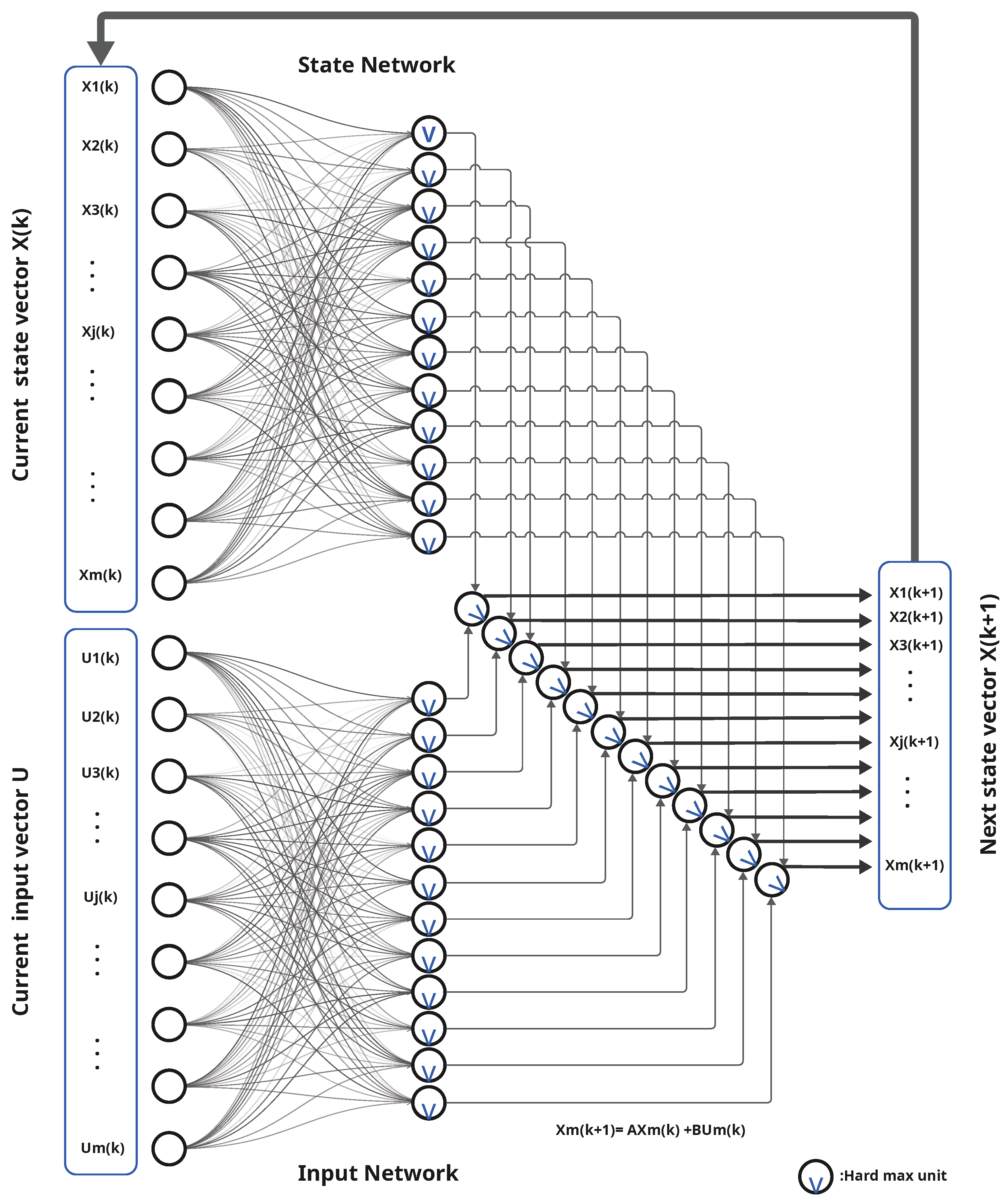
The resulting network is shown in Figure 2. Hence, learning the A and B matrix involves using the matrix form of the neural network weights using standard approaches.

4. Learning the TEG Parameters Using Supervised Learning

In this section, we describe the algorithm to learn the parameters of the dater representation, i.e., the state matrix A and the input matrix B. Since the system state equation expressed in the dater domain is equivalent to a neural network, we develop algorithms similar to the feed-forward and back-propagation in MLPs.

4.1. Problem Statement

Before introducing the learning algorithm, we first formally state the learning problem. To this end, we assume that a TEG of the underlying system, i.e., the number of places and transitions along with the corresponding bipartite graph, is given. Also, we assume that a dataset consisting of ν = 1 N tuples of ( x ν ( k ) , u ν ( k ) , x ν ( k + 1 ) ) has been extracted from the system. Then, we define a neural network equivalent to the dater representation, where the components of the matrices A and B are the weights of the neural network. The task of learning is to learn these weights by minimizing the loss function:
min A , B   L 1   = min A , B i = 1 N x ^ i ( k + 1 ) x i ( k + 1 )

4.2. Learning Algorithm

Our proposed learning scheme can be divided into three steps: (1) forward pass through the network to predict the outputs based on inputs and current parameter values, (2) loss function calculation according to (20), and (3) back-propagating the error through the network to update the network’s parameters. The steps are repeated until a target acceptable error is achieved. The overall algorithm is given in Algorithm 1.
Algorithm 1 Petri net supervised learning.
Require: 
Dataset D = { ( X , u , X ) }
Ensure: 
State matrix A, Input matrix B
  1:
A 1 | Q | × | Q |                     ▹ Initialize with −1
  2:
B 1 | Q | × | U |
  3:
for epoch = 1 to N do
  4:
      for each ( X , u , X ) in D  do
  5:
          X ^ F o r w a r d P a s s ( X , u )                ▹ See Algorithm 2
  6:
          error L 1 ( X , X ^ )
  7:
         Backpropagation( A , B , error)                ▹ See Algorithm 3
  8:
      end for
  9:
end for
10:
return  A , B

4.3. Network Architecture and Tracing

As we deduced in Section 3.5, the Petri net state equation expressed in the data domain is equivalent to two parallel one-layer perceptron networks. Hence, in every network, a transfer function f ( x ) = ( 1 , x ) is applied to the neurons’ activation and then, element-wise, fed into a hard-max unit. We define the first state perceptron network NA with n inputs and m outputs, and NB , and the input perceptron network with u inputs and m outputs.
The above architecture provides the peculiarity that, due to the hard-max operator, only one weight is responsible for the value of the output. Hence, to speed up training, it is advisable to keep track of the history of the path leading to the output value. For example, when computing the hard-max between A x and B u , we can memorize if the current output results from the multiplication A by x or B by u. Since the max operation is element-wise, we can go back in time and determine which weight, when multiplied by the input, gave the max value and proceeded to the max unit. The trace can be used within the back-propagation as given in Algorithm 2.

4.4. Back-Propagation

Once the error is calculated using Equation (20), the algorithm analyzes the path of every component of the output and adjusts the weight of the source of the error. As we previously stated, with a hard-max, every output component is typically affected by one input. Hence, the trace of the path is essentially employed for the back-propagation. We note that alternative approaches using the Gumbel–Softmax distribution [42] for the back-propagation have been explored without notable improvements. Hence, we resort to Algorithm 3.
Algorithm 2 Forward propagation in max-plus algebra.
Require: 
Input vector X, control input u
Ensure: 
Prediction vector Y
  1:
Initialize weight matrices A and B
  2:
for each perceptron p i a in N A  do
  3:
       activation max 1 j n A i j + X j
  4:
       y i a f ( activation )
  5:
      Store activation path
  6:
end for
  7:
for each perceptron p i b in N B  do
  8:
       activation max 1 j u B i j + u j
  9:
       y i b f ( activation )
10:
      Store activation path
11:
end for
12:
for each index i in output Y do
13:
       Y i max ( y i a , y i b )
14:
      Store activation path
15:
end for
16:
return  Y
Algorithm 3 Back-propagation in max-plus algebra.
Require: 
Weight matrices A, B; error vector error; stored activation paths
Ensure: 
Updated matrices A, B
  1:
for each index i in error do
  2:
      if activation path i belongs to N A  then
  3:
           A [ path i ] A [ path i ] η · error i
  4:
      else
  5:
           B [ path i ] B [ path i ] η · error i
  6:
      end if
  7:
end for
  8:
return  A , B

5. Application to Production Scheduling for a Robot Manufacturing Cell

In this section, we demonstrate the application of the proposed approach to a representative case study involving a robot manufacturing cell. We begin by describing the structure and workflow of the manufacturing cell, followed by modelling its dynamics using a coloured timed Petri net. This Petri net is then unfolded into a timed event graph, enabling a representation of system dynamics using max-plus algebra. Leveraging the dater-based description derived from the TEG, we construct a tropical neural network that learns key processing times by observing transition firing patterns within the Petri net.

5.1. Environment Description: Robot Manufacturing Cell

The robot manufacturing cell used in our experiments is located in our laboratory and has been previously described in detail in [43,44]. As shown in Figure 3, the cell consists of two robots, three processing stations ( S 1 , S 2 , S 3 ), two input stations ( I B 1 , I B 2 ), and one output station ( O B ). The two robots operate within a shared workspace, requiring mutual exclusion to prevent collisions and resource conflicts during execution.
The cell handles two types of workpieces, W P 1 and W P 2 , each with a unique routing through the processing stations. Specifically, the routings are
W P 1 : I B 1 S 1 S 2 S 3 O B , W P 2 : I B 2 S 2 S 3 S 1 O B .
We model this system as a job shop scheduling problem (JSSP) due to its structured sequencing of operations and machine-specific constraints. In the classical formulation, let J = { J 1 , J 2 , , J n } denote the set of jobs and M = { M 1 , M 2 , , M m } the set of machines. Each job J i consists of a sequence of operations O i 1 , O i 2 , , O i k , where each operation O i j must be processed on a specific machine M l M for a known duration p i j R + . The decision variables are the start times S i j of the operations.
The scheduling problem is governed by the following constraints:
S i j + 1 S i j + p i j , i , j
S i j S k l + p k l or S k l S i j + p i j , ( i , j ) ( k , l ) with M ( O i j ) = M ( O k l ) ,
C max = max i , j ( S i j + p i j ) min
Equation (21) enforces the sequencing of operations within each job, ensuring that an operation can only start after its predecessor has completed. Equation (22) imposes machine capacity constraints by preventing overlapping operations on the same machine, thus maintaining mutual exclusivity. The objective, expressed in Equation (23), is to minimize the makespan C max , defined as the total completion time of all scheduled operations.
This formulation captures the core temporal and resource dependencies of the robot manufacturing cell. While minimizing makespan is a classical and important scheduling objective, it is not the primary focus of this study. Instead, our emphasis lies on extracting and understanding key temporal characteristics of the system based on event observation, which paves the way for model-based reinforcement learning and enhanced state-value estimation.
To reach this goal, we start by representing the system behaviour using a coloured timed Petri net (CTPN). The timing logic—including processing and transport times—is embedded within the simulation environment but remains hidden from the learning algorithm. These theoretical timing values, summarized in Table 1, serve as ground truth for evaluating our approach.
The matrix T represents the robot transport time (in seconds) between working stations S 1 , S 2 , and S 3 , where T i j is the time to move from station S i to station S j . Diagonal entries are zero since no transport is needed within the same station:
T = S 1 S 2 S 3 S 1 0 2 4 S 2 2 0 3 S 3 4 3 0
To extract temporal patterns from system execution, we monitor the firing behaviour of critical transitions in the CTPN. These events are transformed into a temporal signal using the dater representation, which serves as input to a tropical neural network. The objective is to reconstruct theoretical timing data purely from observed events and infer emergent timing metrics such as waiting durations, inter-event delays, and synchronization latencies caused by resource contention.
The robot manufacturing cell thus presents a rich, real-world scheduling environment characterized by concurrency, sequencing, and transport delays. By capturing its logic with a coloured timed Petri net and analysing its behaviour through tropical learning, we lay the groundwork for future explainable, model-based reinforcement learning approaches.
In the next section, we formally introduce the coloured timed Petri net representation of the manufacturing cell and detail how its structural and temporal properties are encoded for simulation and learning.

5.2. Modelling Using Coloured Petri

We model the robotic manufacturing cell as a coloured timed Petri net (CTPN), extending our previous work [1] where we demonstrated the effectiveness of Petri nets in modelling discrete event systems. The CTPN captures the dynamics of the job shop scheduling problem and also serves as a simulation environment for reinforcement learning. In this setup, the RL agent’s action space corresponds to the controllable transitions, and the observation space is defined by the current marking of the net.
The system’s state evolves through the firing of transitions in the CTPN model, which distinguishes four types: autonomous, controllable, coloured, and timed. All transitions share a fundamental requirement: each upstream place must contain at least one token. Autonomous transitions fire immediately when this condition is satisfied. Controllable transitions additionally require an external trigger, such as a decision from a reinforcement learning agent. Coloured transitions are enabled only when the token’s colour matches the transition’s specified colour, enforcing correct job–machine routing. Timed transitions become eligible to fire only after the token has remained in the upstream place for a predefined sojourn time, capturing the system’s temporal dynamics.
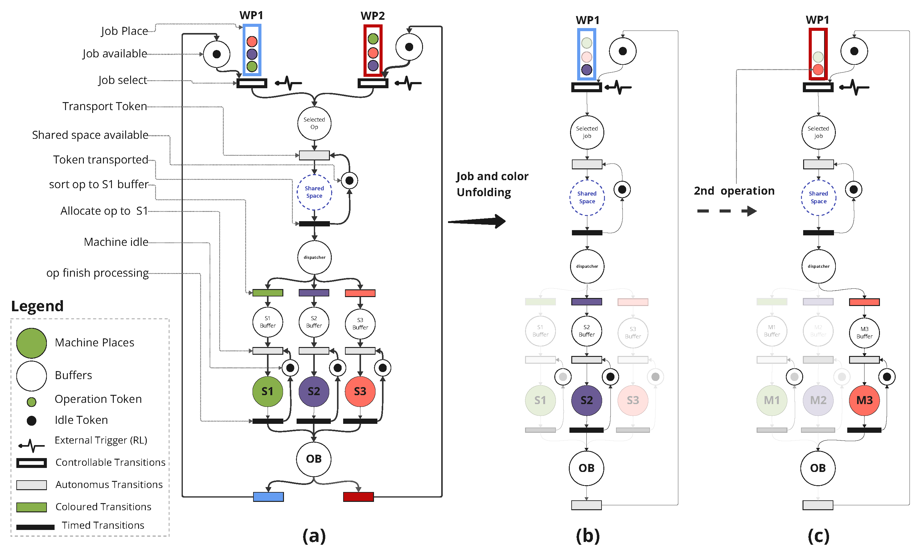
As depicted in Figure 4, the CTPN of the robotic manufacturing cell begins with job places representing workpieces WP1 and WP2. Each workpiece is modelled as a job requiring three sequential operations, represented by coloured tokens encoding a ( job ,   machine ) tuple. The job identifier ensures traceability, while the machine tag directs the operation to the appropriate machine. The process begins with a job-available places, which enforces precedence constraints by ensuring that only one operation per job is active at a time. A job-selection transition fires if the job is idle, a token is present, and an external trigger, such as a reinforcement learning (RL) decision, is provided. If a shared space is available, the robot transfers the selected workpiece to the next stage via a timed transport transition, simulating physical movement delays. Based on the token’s colour, the workpiece is routed to the correct machine buffer. A machine-allocation transition then fires immediately if the machine is available, controlled by a machine-idle place to guarantee exclusive machine access. Once the processing time elapses, an operation-finish timed transition fires, and the token is returned to the job-available place, enabling the selection of the next operation in the job sequence. This temporal progression ensures that precedence, routing, resource availability, and timing constraints are respected throughout the execution of the schedule.
As previously outlined, the goal is to represent the system as a max-plus linear equation, which will later be transformed into a tropical neural network. To achieve this, the Petri net must be a timed event graph (TEG), also known as a choice-free net. As the name suggests, all choices and resource concurrency must be eliminated. This translates to the structural requirement that every place has exactly one input and one output transition [45]. To satisfy this constraint, we apply unfolding techniques, which are detailed in the following paragraph.

5.3. Unfolding Coloured Timed Petri Net into Timed Event Graph

The goal is to transform the CTPN into a choice-free net to be able to describe it with max-plus algebra. To achieve this, all points of resource concurrency must be eliminated. In Figure 4a, we identify three locations where the choice-free net requirement is violated: (i) the selected operation place has two input transitions, (ii) the dispatching place has three output transitions, and (iii) the output buffer (OB) place has three input and two output transitions. These structural conflicts must be resolved to conform to the choice-free constraint, which requires each place to have exactly one input and one output.
We use the unfolding technique introduced in Section 3.2 to unfold the coloured Petri net in two stages: at the job level and at the machine level.
The first stage involves unfolding the net based on the job. For each job—representing a workpiece—we extract an associated timed event graph (TEG). This is feasible because an external trigger, originating from the reinforcement learning agent or another decision-making component, initiates a sequence of events linked to the job, beginning with the job selection action. An illustration of the resulting TEG from this job-level unfolding is shown in Figure 4b.
Although machines introduce additional sources of concurrency at the level of the dispatching places, Figure 4b, demonstrates that at the step-wise level, only a single route is available for each token based on its colour. As a result, the TEG conditions remain satisfied, and the system’s determinism at this level is preserved.
Once all conflicts are resolved, the model is ready for the next stage, which involves extracting the data and control equations that describe the behaviour of the robotic manufacturing cell.

5.4. Dater and Counter Representations of the Manufacturing Cell

We consider a manufacturing cell processing two jobs, each with n = 3 sequential operations. Our goal is to identify key timing parameters by logging only essential transitions: select (external trigger), dispatch (material transfer), and process (completion). These capture critical timing events.
To model timing modularly and scalably, we adopt a token-centric approach, where each token represents a job operation flowing through the Petri net. Instead of tracking global states, we focus on the local evolution of individual tokens.
This ensures modularity by treating tokens uniformly, scalability by handling varying job lengths and routes, and interpretability by reducing system behaviour to a structured state-space per token, aiding parameter identification and diagnostics.
We start learning at the operation-token level, then aggregate to the job level, and finally to the system level with multiple concurrent jobs. This hierarchical modelling enhances modularity, scalability, and interpretability of the scheduling system.
Consider a single operation represented by a token with the state vector at a discrete time step k defined as
X ( k ) = x s ( k ) x d ( k ) x p ( k ) ,
where x s ( k ) is the selection time, x d ( k ) the dispatch time after transport delay t transfer , and x p ( k ) the processing completion time after processing delay t p . The operation evolves according to the max-plus algebraic equations. The dater formulation is
x s i ( j ) ( k ) = u j i ( k ) 0 , i = 1 x p i 1 ( j ) ( k 1 ) , i > 1 x d i ( j ) ( k ) = x s i ( j ) ( k 1 ) t transfer x p i ( j ) ( k ) = x d i ( j ) ( k 1 ) t p j i
And the counter formulation is
n s i ( j ) ( t ) = max u j i ( t ) , 0 , i = 1 n p i 1 ( j ) ( t ) , i > 1 n d i ( j ) ( t ) = n s i ( j ) ( t t transfer ) n p i ( j ) ( t ) = n d i ( j ) ( t t p j i )
The dater formulation can be compactly written in state-space form as
X ( k + 1 ) = A X ( k ) B u ( k ) ,
with
A = ε ε ε t transfer ε ε ε t p ε , B = 0 ε ε ε ε ε ε ε ε ,
Extending this framework to a job j composed of three sequential operations, the dater is given by Equation (26) and the counter by Equation (27) for the first job:
x s 1 ( j ) ( k ) = u j 1 ( k ) 0 x d 1 ( j ) ( k ) = x s 1 ( j ) ( k ) t transfer IB S 1 x p 1 ( j ) ( k ) = x d 1 ( j ) ( k ) t p 11 x s 2 ( j ) ( k ) = u j 2 ( k ) x p 1 ( j ) ( k 1 ) x d 2 ( j ) ( k ) = x s 2 ( j ) ( k ) t transfer S 1 S 2 x p 2 ( j ) ( k ) = x d 2 ( j ) ( k ) t p 12 x s 3 ( j ) ( k ) = u j 3 ( k ) x p 2 ( j ) ( k 1 ) x d 3 ( j ) ( k ) = x s 3 ( j ) ( k ) t transfer S 2 S 3 x p 3 ( j ) ( k ) = x d 3 ( j ) ( k ) t p 13
n s 1 ( j ) ( t ) = max u j 1 ( t ) , 0 n d 1 ( j ) ( t ) = n s 1 ( j ) t t transfer IB S 1 n p 1 ( j ) ( t ) = n d 1 ( j ) t t p j 1 n s 2 ( j ) ( t ) = max u j 2 ( t ) , n p 1 ( j ) ( t ) n d 2 ( j ) ( t ) = n s 2 ( j ) t t transfer S 1 S 2 n p 2 ( j ) ( t ) = n d 2 ( j ) t t p j 2 n s 3 ( j ) ( t ) = max u j 3 ( t ) , n p 2 ( j ) ( t ) n d 3 ( j ) ( t ) = n s 3 ( j ) t t transfer S 2 S 3 n p 3 ( j ) ( t ) = n d 3 ( j ) t t p j 3
The job state vector aggregates the individual operation states as
X ( j ) ( k ) = X 1 ( j ) ( k ) X 2 ( j ) ( k ) X 3 ( j ) ( k )
The intra-job dependencies and time delays are captured in a block-structured system matrix, A j , representing the cascaded operation dynamics.
Finally, for multiple jobs j = 1 , 2 running concurrently, the overall system state vector concatenates the job vectors:
X ( k ) = X ( 1 ) ( k ) X ( 2 ) ( k ) R max 18 ,
with the overall dynamics
X ( k + 1 ) = A X ( k ) B u ( k ) ,
where A and B are block matrices composed of the job-specific matrices A j and B j , capturing both intra-job sequences and inter-job resource constraints.
A j = ε ε ε ε ε ε ε ε ε t transfer ε ε ε ε ε ε ε ε ε t p j 1 ε ε ε ε ε ε ε ε ε 0 ε ε ε ε ε ε ε ε ε t transfer ε ε ε ε ε ε ε ε ε t p j 2 ε ε ε ε ε ε ε ε ε 0 ε ε ε ε ε ε ε ε ε t transfer ε ε ε ε ε ε ε ε ε t p j 3 ε B j = 0 ε ε ε ε ε ε ε ε ε ε ε ε ε ε ε ε ε ε ε ε ε ε ε ε ε ε ε ε ε 0 ε ε ε ε ε ε ε ε ε ε ε ε ε ε ε ε ε ε ε ε ε ε ε ε ε ε ε ε ε 0 ε ε ε ε ε ε ε ε ε ε ε ε ε ε ε ε ε ε ε ε
This hierarchical modular structure is modular, as each job’s dynamics lie in diagonal blocks enabling independent control; scalable, as additional jobs extend matrices A and B naturally; and interpretable, as the max-plus algebra formulation captures the timing and ordering constraints explicitly in a transparent mathematical model.

6. Results and Discussion

In this section, we employ supervised learning to train the tropical neural network to reconstruct the system matrices A and B. We begin with a general case where all values are randomly generated, and then we validate it with the robot cell case.

6.1. Dataset Generation and Training

In the first step, we begin by randomly generating and freezing the system matrices A and B. With these matrices frozen, we generate random input–state pairs ( x ( k ) , u ( k ) ) , and compute the next states x ( k + 1 ) according to the max-plus system dynamics:
x ( k + 1 ) = A x ( k ) B u ( k ) ,
After collecting a dataset of triplets ( x ( k ) , u ( k ) , x ( k + 1 ) ) , the goal is to reconstruct the original matrices A and B from these transitions alone.
In the second step, after validating the approach on randomly generated data, we apply it to a robotic cell modelled by a coloured timed Petri net. Here, the dynamics encoded in the simulation implicitly define the matrices A and B, and we extract triplets ( x ( k ) , u ( k ) , x ( k + 1 ) ) from simulation runs.
The state vector x ( k ) records the firing times of key transitions select, dispatch, and process at their k-th occurrence. Since each job consists of three operations, we stack three such vectors per job to represent their temporal progression. The control input u ( k ) corresponds to a scheduler’s input, either by a human operator or by a scheduling algorithm, which selects a transition to fire, triggering the next operation.
As the agent explores different policies during training, it generates diverse triplets used to train a tropical neural network via max-plus regression. Data collection is performed in parallel with training; for example, over 1000 simulation steps, the agent may complete 65 episodes, each yielding multiple triplets. This setup ensures wide coverage of the state–action space and enables the network to learn the system’s timing behaviour and structural constraints.

6.2. Results

We begin with the general case to evaluate the foundational behaviour of the proposed approach. First, we analyse the training dynamics of the learning algorithm. Then, we assess its robustness to noise in the dataset and its adaptability to variations in processing times.
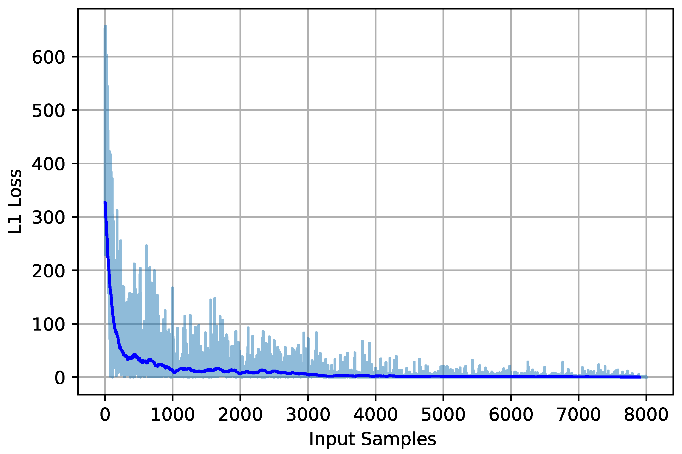
The primary hyperparameter in the training dynamics of the learning algorithm is the learning rate α . Its value was determined through an empirical investigation where we evaluated a range of values, specifically 10 1 , 10 2 , and 10 3 , and assessed their impact on convergence speed and training stability. Figure 5 shows the supervised training results using a learning rate α = 10 2 on a dataset of 10,000 randomly generated samples. The plot demonstrates rapid convergence of the L1 loss, indicating that the model effectively captures the underlying max-plus structure.
As shown in Figure 5, the loss stabilizes after approximately 1000 samples, reflecting the influence of the learning rate α . The loss corresponds to the cumulative element-wise error between the predicted x ( k + 1 ) and the ground truth x ( k + 1 ) from the dataset. This behaviour illustrates a key trade-off: a higher learning rate leads to faster adaptation, allowing new data to have a stronger impact on model updates. However, it also increases sensitivity to noise, potentially resulting in unstable training. Conversely, a lower learning rate introduces a form of momentum that smooths updates, promoting robustness but at the cost of slower learning and delayed convergence.
Following the general convergence analysis, we further investigate the convergence behaviour of the learned system matrices A and B. To quantitatively evaluate performance, we employ a similarity metric to compare the learned matrices A ˜ and B ˜ against their reference counterparts A ref and B ref . Specifically, we use the Minkowski distance of order 2 ( p = 2 ):
D ( x , y ) = i = 1 n | x i y i | p 1 p ,
where x and y denote the vectorized forms of the matrices. This metric provides a rigorous quantitative measure, enabling us to track how closely the learned parameters approximate the ground truth throughout training.
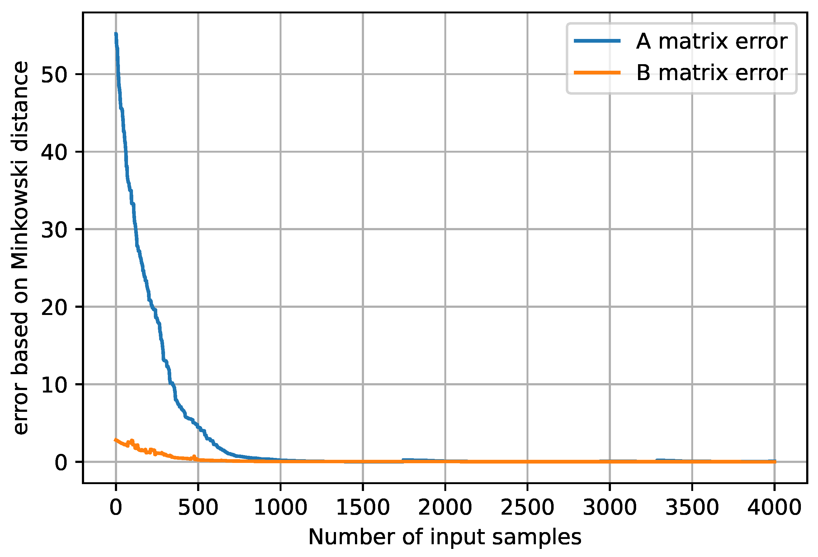
Figure 6 presents the empirical error curves for both matrices. Both distance metrics decrease rapidly, demonstrating the effective learning capability of the proposed approach. Notably, due to the structural properties of the B matrix and its initialization scheme, its error converges faster than that of the A matrix, which includes processing time parameters and exhibits more complexity.
In Figure 7, we present a detailed element-wise analysis of the system’s prediction performance. The process begins by selecting two random vectors: x representing the current state, and u representing the control input. These vectors are then multiplied by the reference system matrices A and B to compute the reference next state, denoted as x ref + :
x ref + = A x + B u .
Throughout the training procedure, snapshots are captured by applying the same input and state vectors to the intermediate learned system matrices A ^ and B ^ . The resulting predicted next states, x ^ + , are logged at each training step to track the evolution of the learned model and its convergence towards the reference dynamics:
x ^ + = A ^ x + B ^ u .
The top subplot in Figure 7 illustrates the trajectory of the reference next state vector x k + 1 alongside the evolving predictions over the course of training. This visualization highlights the overall convergence behaviour across all state elements.
The bottom four subplots provide a focused view on the evolution of specific state components—namely x 3 , x 4 , x 5 , and x 6 . These graphs clearly demonstrate that as training progresses, the predicted values increasingly align with the reference states, indicating effective learning and improved accuracy of the model.
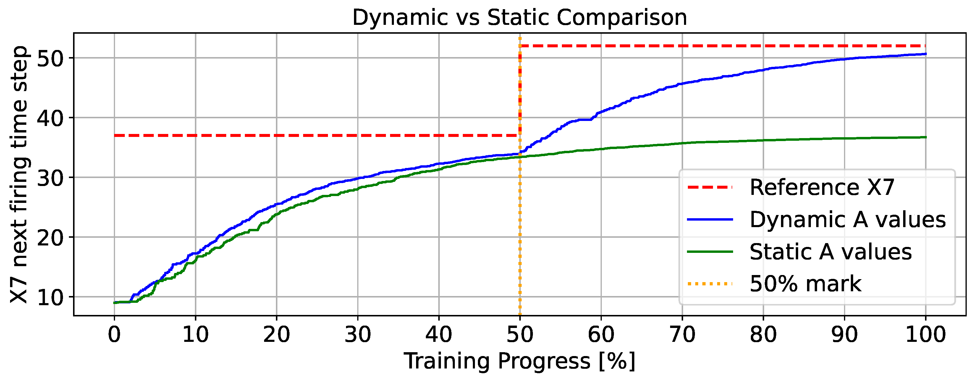
Next, we evaluate the adaptability of our approach to dynamic changes within the system. To this end, we simulate a scenario where the timing values in the A matrix are altered midway through training. This change represents shifts in processing times due to factors such as tool wear (leading to slower operations) or transportation bottlenecks, causing delays. Specifically, for the first 50% of the training process, the A matrix remains constant. At the 50% mark, all timing values in the A matrix are scaled to 150% of their original values. This sudden change tests the agent’s ability to adapt to evolving temporal parameters in the environment.
Figure 8 illustrates the system’s response to a change in the reference dynamics. The red curve represents the reference date for a given transition, specifically, the expected firing of transition seven in the next time step. Initially, this transition is predicted to fire at time step 39, based on the initial inputs x ref and U ref , and their multiplication with the reference matrices A ref and B ref .
During the first half of training (before the 50% training mark), the system learns the matrix A based on observed data, which is generated using the original reference time and input matrices. The blue and green curves show the evolution of the predicted values obtained by multiplying x ref and U ref with the intermediate versions of the learned A matrix throughout training. At the 50% training mark, the reference matrix A ref is modified to be 150% of its original value. This causes a step change in the target value x k + 1 (red curve), shifting the expected firing time from step 39 to step 51.
In the static case, where the reference matrix A is frozen after the change, the green curve fails to track the new reference and continues along the outdated trajectory. Conversely, in the adaptive case, the system continues updating the matrix A, and the blue curve successfully adapts to the new reference, eventually aligning with the updated target.
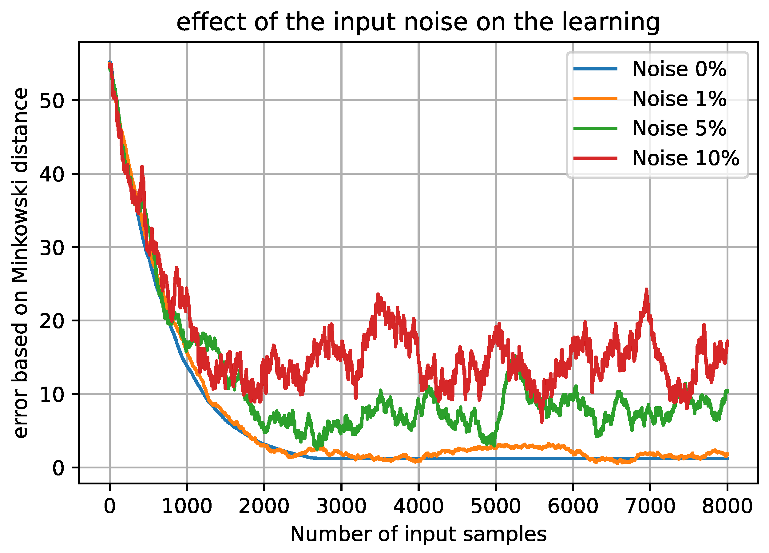
Robustness of the model is evaluated by introducing Gaussian noise with zero mean and a variance scaled from 1% to 10% relative to the original label magnitudes. Table 2 presents a comprehensive summary of the resulting Minkowski distances calculated between the learned and reference time matrices, as well as between their corresponding predicted next states x ( k + 1 ) , under these varying noise levels. This analysis provides insight into the sensitivity of the model’s predictions to increasing noise perturbations.
Figure 9 illustrates the learning behaviour under these noisy conditions. Despite the incremental increase in noise variance, the network’s convergence remains stable, demonstrating strong robustness of the proposed approach. As expected, the reconstruction error increases with higher noise levels, particularly evident in the predicted state errors, which amplify the effect of noisy labels. This analysis confirms that while noise degrades absolute accuracy, the model maintains consistent learning dynamics and resilience in the presence of realistic data perturbations.
Finally, we validate the approach by testing it on a robotic cell. Unlike the general case, this setup requires a specialized initialization procedure. In typical production environments, the initial state vector x 0 is often initialized with zeros to indicate that all processes start at time zero:
x 0 = 0 0 0
However, this introduces a critical problem. If all elements of the system matrix A are initialized with the max-plus identity element , then the max-plus matrix multiplication
A x 0
yields a vector filled entirely with . This occurs because
a i j = max j ( a i j + x j ) =
This outcome not only prevents any meaningful progression in learning but also blocks gradient flow during back-propagation, as no finite values propagate through the computational graph.
To overcome this limitation, it is essential to initialize the matrix A with some finite values. These finite entries enable meaningful max-plus algebraic computations and allow gradients to flow during training, thus facilitating learning. Since the production plan’s structure is assumed to be known a priori, we initialize the timing elements of A , corresponding to processing and transport delays, using the max-plus neutral element e = 0 , which acts as the additive identity in max-plus algebra.
An example of the learned matrix A for Job 1 is presented below. According to the max-plus dater equation in (24), the elements A 3 , 2 , A 6 , 5 , and A 9 , 8 correspond to the processing times of the operations in Job 1. Specifically,
A 3 , 2 = p 11 = 10 , A 6 , 5 = p 12 = 20 , A 9 , 8 = p 13 = 30 ,
which represent the durations of processing the operations at Station 1, Station 2, and Station 3, respectively.
Additionally, the elements A 2 , 1 , A 5 , 4 , and A 8 , 7 represent the transport times between successive stages of the job. Specifically,
A 2 , 1 = t IB S 1 = 0 , A 5 , 4 = t S 1 S 2 = 2 , A 8 , 7 = t S 2 S 3 = 3 ,
where t IB S 1 denotes the transport time from the input buffer (IB) to Station 1, t S 1 S 2 denotes the transport time from Station 1 to Station 2, and t S 2 S 3 denotes the transport time from Station 2 to Station 3.
A ˜ = 1 1 1 1 1 1 1 1 1 0.01 1 1 1 1 1 1 1 1 1 9.96 1 1 1 1 1 1 1 1 1 0.01 1 1 1 1 1 1 1 1 1 1.96 1 1 1 1 1 1 1 1 1 19.85 1 1 1 1 1 1 1 1 1 0.01 1 1 1 1 1 1 1 1 1 2.95 1 1 1 1 1 1 1 1 1 29.93 1
We highlight that the various timing values embedded in the matrix A correspond closely to the predefined processing and transport times of the system. This alignment demonstrates that the proposed approach successfully identifies key system timing parameters solely from input–output observations. Such accurate recovery of timing characteristics validates the effectiveness of the model and confirms its potential for reliable scheduling and control in practical industrial settings.

7. Conclusions

The choice of adequate, adjustable modelling tools is a stepping stone in the optimization of various industrial applications. In this work, we proposed a modelling approach based on timed event graphs that can be trained using a standard approach from the machine learning domain. To this end, we establish equivalence relations between timed event graphs, and their dater and counter representation using max-plus algebra and specifically designed neural networks. We propose learning algorithms designed to adjust the network parameters based on datasets obtained from the system at hand. We employ our approach to scheduling operations within a robot manufacturing cell where the results underscore the applicability and performance of the approach.
Future research will be concerned with more efficient methods to utilize the sample in learning the timing matrix A by using the temperature gradient method. Furthermore, we will integrate our learnable TEG into reinforcement learning loops, in which the TEG serves as a model of the environment similar to model-based RL.

Author Contributions

M.S.A.H., S.L. and A.S. contributed as follows: Conceptualization, M.S.A.H., S.L. and A.S.; Methodology, M.S.A.H., S.L. and A.S.; Software, M.S.A.H. and S.L.; Validation, M.S.A.H., S.L. and A.S.; Formal analysis, M.S.A.H., S.L. and A.S.; Investigation, M.S.A.H. and S.L.; Resources, A.S.; Data curation, M.S.A.H. and S.L.; Writing original draft preparation, M.S.A.H., S.L. and A.S.; Writing review and editing, M.S.A.H., S.L. and A.S.; Visualization, M.S.A.H. and S.L.; Supervision, A.S.; Project administration, A.S. All authors have read and agreed to the published version of the manuscript.

Funding

This publication is funded by the Open Access Publication Fund of South Westphalia University of Applied Sciences.

Data Availability Statement

The synthetic data used in this study were generated by probing events in our PetriRL simulation environment. The PetriRL Python package is available at https://pypi.org/project/petrirl/ (accessed on 9 September 2025), and all scripts used to generate and process the data are available at https://github.com/Sofiene-Uni/Petri-MaxPlus (accessed on 9 September 2025).

Conflicts of Interest

The authors declare no conflicts of interest.

References

  1. Lassoued, S.; Schwung, A. Introducing PetriRL: An innovative framework for JSSP resolution integrating Petri nets and event-based reinforcement learning. J. Manuf. Syst. 2024, 74, 690–702. [Google Scholar] [CrossRef]
  2. Zhang, L.G.; Li, Z.L.; Chen, Y.Z. Hybrid petri net modeling of traffic flow and signal control. In Proceedings of the 2008 International Conference on Machine Learning and Cybernetics, Kunming, China, 12–15 July 2008; Volume 4, pp. 2304–2308. [Google Scholar] [CrossRef]
  3. Cavone, G.; Dotoli, M.; Seatzu, C. A Survey on Petri Net Models for Freight Logistics and Transportation Systems. IEEE Trans. Intell. Transp. Syst. 2018, 19, 1795–1813. [Google Scholar] [CrossRef]
  4. Shih, H.M.; Sekiguchi, T. A timed Petri net and beam search based online FMS scheduling system with routing flexibility. In Proceedings of the IEEE International Conference on Robotics and Automation, Sacramento, CA, USA, 9–11 April 1991; pp. 2548–2553. [Google Scholar]
  5. Jensen, K.; Rozenberg, G. High-Level Petri Nets: Theory and Application; Jensen, K., Rozenberg, G., Eds.; Springer: Berlin, Germany; New York, NY, USA, 1991. [Google Scholar]
  6. Baccelli, F.; Cohen, G.; Olsder, G.J.; Quadrat, J.P. Synchronization and Linearity: An Algebra for Discrete Event Systems; Wiley series in probability and mathematical statistics; J. Wiley & Sons: Chichester, UK; New York, NY, USA, 1992; pp. 99–151. [Google Scholar]
  7. Cohen, G.; Moller, P.; Quadrat, J.P.; Viot, M. Algebraic tools for the performance evaluation of discrete event systems. Proc. IEEE 1989, 77, 39–85. [Google Scholar] [CrossRef]
  8. Latorre-Biel, J.I.; Faulín, J.; Juan, A.A.; Jiménez-Macías, E. Petri Net Model of a Smart Factory in the Frame of Industry 4.0. IFAC-PapersOnLine 2018, 51, 266–271. [Google Scholar] [CrossRef]
  9. Hatono, I.; Yamagata, K.; Tamura, H. Modeling and online scheduling of flexible manufacturing systems using stochastic Petri nets. IEEE Trans. Softw. Eng. 1991, 17, 126–132. [Google Scholar] [CrossRef]
  10. Long, F.; Zeiler, P.; Bertsche, B. Modelling the production systems in industry 4.0 and their availability with high-level Petri nets. IFAC-PapersOnLine 2016, 49, 145–150. [Google Scholar] [CrossRef]
  11. Ritter, G.X.; Sussner, P. An introduction to morphological neural networks. In Proceedings of the 13th International Conference on Pattern Recognition, Vienna, Austria, 25–29 August 1996; IEEE: Las Vegas, NV, USA, 1996; Volume 4, pp. 709–717. [Google Scholar]
  12. Sussner, P.; Esmi, E.L. Morphological perceptrons with competitive learning: Lattice-theoretical framework and constructive learning algorithm. Inf. Sci. 2011, 181, 1929–1950. [Google Scholar] [CrossRef]
  13. Charisopoulos, V.; Maragos, P. Morphological perceptrons: Geometry and training algorithms. In Mathematical Morphology and Its Applications to Signal and Image Processing, Proceedings of the 13th International Symposium, ISMM 2017, Fontainebleau, France, 15–17 May 2017; Proceedings 13; Springer: Berlin/Heidelberg, Germany, 2017; pp. 3–15. [Google Scholar]
  14. Maragos, P.; Charisopoulos, V.; Theodosis, E. Tropical geometry and machine learning. Proc. IEEE 2021, 109, 728–755. [Google Scholar] [CrossRef]
  15. Charisopoulos, V.; Maragos, P. A Tropical Approach to Neural Networks with Piecewise Linear Activations. arXiv 2018, arXiv:1805.08749. [Google Scholar]
  16. Zhang, L.; Naitzat, G.; Lim, L.H. Tropical Geometry of Deep Neural Networks. In Proceedings of the International Conference on Machine Learning, Stockholm, Sweden, 10–15 July 2018; pp. 5824–5832. [Google Scholar]
  17. De Schutter, B.; van den Boom, T.J.; Verdult, V. State space identification of max-plus-linear discrete event systems from input-output data. In Proceedings of the 41st IEEE Conference on Decision and Control, Las Vegas, NV, USA, 10–13 December 2002; IEEE: New York, NY, USA, 2002; Volume 4, pp. 4024–4029. [Google Scholar]
  18. Farahani, S.S.; van den Boom, T.; De Schutter, B. Exact and approximate approaches to the identification of stochastic max-plus-linear systems. Discret. Event Dyn. Syst. 2014, 24, 447–471. [Google Scholar] [CrossRef]
  19. Li, Z.; Wang, Y.; Wang, K.S. Intelligent predictive maintenance for fault diagnosis and prognosis in machine centers: Industry 4.0 scenario. Adv. Manuf. 2017, 5, 377–387. [Google Scholar] [CrossRef]
  20. Rivas, A.; Fraile, J.M.; Chamoso, P.; González-Briones, A.; Sittón, I.; Corchado, J.M. A predictive maintenance model using recurrent neural networks. In Proceedings of the 14th International Conference on Soft Computing Models in Industrial and Environmental Applications (SOCO 2019), Seville, Spain, 13–15 May 2019; Proceedings 14. Springer: Berlin/Heidelberg, Germany, 2020; pp. 261–270. [Google Scholar]
  21. Usuga Cadavid, J.P.; Lamouri, S.; Grabot, B.; Pellerin, R.; Fortin, A. Machine learning applied in production planning and control: A state-of-the-art in the era of industry 4.0. J. Intell. Manuf. 2020, 31, 1531–1558. [Google Scholar] [CrossRef]
  22. Wu, W.; Ma, Y.; Qiao, F.; Gu, X. Data mining-based dynamic scheduling approach for semiconductor manufacturing system. In Proceedings of the 2015 34th Chinese Control Conference (CCC), Hangzhou, China, 28–30 July 2015; IEEE: New York, NY, USA, 2015; pp. 2603–2608. [Google Scholar]
  23. Priore, P.; Ponte, B.; Puente, J.; Gómez, A. Learning-based scheduling of flexible manufacturing systems using ensemble methods. Comput. Ind. Eng. 2018, 126, 282–291. [Google Scholar] [CrossRef]
  24. Huang, B.; Wang, W.; Ren, S.; Zhong, R.Y.; Jiang, J. A proactive task dispatching method based on future bottleneck prediction for the smart factory. Int. J. Comput. Integr. Manuf. 2019, 32, 278–293. [Google Scholar] [CrossRef]
  25. Hu, L.; Liu, Z.; Hu, W.; Wang, Y.; Tan, J.; Wu, F. Petri net-based dynamic scheduling of flexible manufacturing system via deep reinforcement learning with graph convolutional network. J. Manuf. Syst. 2020, 55, 1–14. [Google Scholar] [CrossRef]
  26. Thomas, T.E.; Koo, J.; Chaterji, S.; Bagchi, S. Minerva: A reinforcement learning-based technique for optimal scheduling and bottleneck detection in distributed factory operations. In Proceedings of the 2018 10th International Conference On Communication Systems & Networks, Bengaluru, India, 3–7 January 2018; IEEE: New York, NY, USA, 2018. [Google Scholar]
  27. Waschneck, B.; Reichstaller, A.; Belzner, L.; Altenmüller, T.; Bauernhansl, T.; Knapp, A.; Kyek, A. Optimization of global production scheduling with deep reinforcement learning. Procedia CIRP 2018, 72, 1264–1269. [Google Scholar] [CrossRef]
  28. Zhang, W.; Dietterich, T.G. A reinforcement learning approach to job-shop scheduling. In Proceedings of the IJCAI, Montreal, QC, Canada, 20–25 August 1995; Volume 95, pp. 1114–1120. [Google Scholar]
  29. Gabel, T.; Riedmiller, M. Adaptive reactive job-shop scheduling with reinforcement learning agents. Int. J. Inf. Technol. Intell. Comput. 2008, 24, 14–18. [Google Scholar]
  30. Hameed, M.S.A.; Schwung, A. Reinforcement learning on job shop scheduling problems using graph networks. arXiv 2020, arXiv:2009.03836. [Google Scholar]
  31. Hameed, M.S.A.; Schwung, A. Graph neural networks-based scheduler for production planning problems using reinforcement learning. J. Manuf. Syst. 2023, 69, 91–102. [Google Scholar] [CrossRef]
  32. Park, J.; Chun, J.; Kim, S.H.; Kim, Y.; Park, J. Learning to schedule job-shop problems: Representation and policy learning using graph neural network and reinforcement learning. Int. J. Prod. Res. 2021, 59, 3360–3377. [Google Scholar] [CrossRef]
  33. Mejía, G.; Caballero-Villalobos, J.P.; Montoya, C. Petri Nets and Deadlock-Free Scheduling of Open Shop Manufacturing Systems. IEEE Trans. Syst. Man Cybern. Syst. 2018, 48, 1017–1028. [Google Scholar] [CrossRef]
  34. Reisig, W. Understanding Petri Nets; Springer: Berlin/Heidelberg, Germany, 2013. [Google Scholar]
  35. Moro, A.R.; Yu, H.; Kelleher, G. Hybrid heuristic search for the scheduling of flexible manufacturing systems using Petri nets. IEEE Trans. Robot. Autom. 2002, 18, 240–245. [Google Scholar] [CrossRef]
  36. Jensen, K. Coloured Petri Nets: Basic Concepts, Analysis Methods and Practical Use; Springer: Berlin/Heidelberg, Germany, 1996. [Google Scholar]
  37. Liu, F.; Heiner, M.; Yang, M. An efficient method for unfolding colored Petri nets. In Proceedings of the 2012 Winter Simulation Conference (WSC), Berlin, Germany, 9–12 December 2012; IEEE: New York, NY, USA, 2012; pp. 1–12. [Google Scholar][Green Version]
  38. DiCesare, F.; Harhalakis, G.; Proth, J.M.; Silva Suarez, M.; Vernadat, F.B. Practice of Petri Nets in Manufacturing; Springer: Dordrecht, The Netherlands, 2012. [Google Scholar][Green Version]
  39. Butkovič, P. Max-Linear Systems: Theory and Algorithms; Springer monographs in mathematics; Springer: London, UK, 2010. [Google Scholar][Green Version]
  40. Hornik, K.; Stinchcombe, M.; White, H. Multilayer feedforward networks are universal approximators. Neural Netw. 1989, 2, 359–366. [Google Scholar] [CrossRef]
  41. Parhi, R.; Nowak, R.D. The Role of Neural Network Activation Functions. IEEE Signal Process. Lett. 2020, 27, 1779–1783. [Google Scholar] [CrossRef]
  42. Jang, E.; Gu, S.; Poole, B. Categorical Reparameterization with Gumbel-Softmax. arXiv 2017, arXiv:1611.01144. [Google Scholar] [CrossRef]
  43. Schwung, D.; Csaplar, F.; Schwung, A.; Ding, S.X. An application of reinforcement learning algorithms to industrial multi-robot stations for cooperative handling operation. In Proceedings of the 2017 IEEE 15th International Conference on Industrial Informatics (INDIN), Emden, Germany, 24–26 July 2017; pp. 194–199. [Google Scholar]
  44. Schwung, A.; Schwung, D.; Hameed, M.S.A. Cooperative Robot Control in Flexible Manufacturing Cells. In Proceedings of the 2019 IEEE 17th International Conference on Industrial Informatics (INDIN), Helsinki-Espoo, Finland, 22–25 July 2019; Volume 1, pp. 233–238. [Google Scholar]
  45. Trunk, J.; Cottenceau, B.; Hardouin, L.; Raisch, J. Model decomposition of timed event graphs under periodic partial synchronization: Application to output reference control. Discret. Event Dyn. Syst. 2020, 30, 605–634. [Google Scholar] [CrossRef]
Figure 1. Example of various types of Petri nets: (a) basic Petri net, (b) coloured Petri net, (c) timed coloured Petri net.
Make 07 00100 g001
Figure 2. Max-plus model learning schematic using perceptron.
Make 07 00100 g002
Figure 3. Overview of the experimental test-bed, showing two robots, three processing stations, two input stations, and one output station.
Make 07 00100 g003
Figure 4. The transition from the system’s coloured timed Petri net model to a timed event graph. (a) The full coloured timed Petri net model of the robot cell, (b) the colour and job unfolding into a monochrome Petri net, (c) a depiction of the next step with the next coloured token.
Make 07 00100 g004
Figure 5. Element-wise L1 loss between the predicted and ground truth x ( k + 1 ) during supervised training. The light blue curve shows the actual loss, while the dark blue curve shows its moving average.
Make 07 00100 g005
Figure 6. Training error dynamics for the learned system matrices A and B. The plot shows the decrease in the Minkowski distance between the learned matrices A ˜ , B ˜ and their reference counterparts A ref , B ref over training iterations.
Make 07 00100 g006
Figure 7. Comparison of prediction evolution against the reference values across all eight state segments. The top plot shows the full trajectory, while the bottom subplots detail individual predictions for states x 3 to x 6 .
Make 07 00100 g007
Figure 8. Transition X7 firing time evolution with matrix A changing at 50% training. The dynamic case updates the network to adapt, while the static case keeps the original matrix unchanged.
Make 07 00100 g008
Figure 9. Impact of label noise on the learning performance.
Make 07 00100 g009
Table 1. Processing times (in seconds) for each workpiece at each station. A dash (–) indicates that the station is not used by the corresponding workpiece.
Station W P 1 W P 2
Input station ( I B 1 ) 0
Input station ( I B 2 ) 0
Working station ( S 1 ) 1030
Working station ( S 2 ) 2010
Working station ( S 3 ) 3020
Output station ( O B ) 00
Table 2. Minkowski distances between learned and reference matrices and states for varying noise levels.
Noise LevelMatrix DistanceState Distance
σ = 1 % 2.052.82
σ = 5 % 9.079.59
σ = 10 % 12.9829.78
Disclaimer/Publisher’s Note: The statements, opinions and data contained in all publications are solely those of the individual author(s) and contributor(s) and not of MDPI and/or the editor(s). MDPI and/or the editor(s) disclaim responsibility for any injury to people or property resulting from any ideas, methods, instructions or products referred to in the content.