Automatic Detection of Equatorial Plasma Bubbles in Airglow Images Using Two-Dimensional Principal Component Analysis and Explainable Artificial Intelligence

Abstract

Equatorial plasma bubbles (EPBs) are regions of depleted electron density that form in the Earth’s ionosphere due to Rayleigh–Taylor instability. These bubbles can cause signal scintillation, leading to signal loss and errors in position calculations. EPBs can be detected in images captured by All-Sky Imager (ASI) systems. This study proposes a low-cost automatic detection method for EPBs in ASI data that can be used for both real-time detection and classification purposes. This method utilizes Two-Dimensional Principal Component Analysis (2DPCA) with Recursive Feature Elimination (RFE), in conjunction with a Random Forest machine learning model, to create an Explainable Artificial Intelligence (XAI) model capable of extracting image features to automatically detect EPBs with the lowest possible dimensionality. This led to having a small-sized and extremely fast-trained model that could be used to identify EPBs within the captured ASI images. A set of 2458 images, classified into two categories—Event and Empty—were used to build the database. This database was randomly split into two subsets: a training dataset (80%) and a testing dataset (20%). The produced XAI model demonstrated slightly higher detection accuracy compared to the standard 2DPCA model while being significantly smaller in size. Furthermore, the proposed model’s performance has been evaluated and compared with other deep learning baseline models (ResNet18, Inception-V3, VGG16, and VGG19) in the same environment.

1. Introduction

Equatorial plasma bubbles (EPBs) are common phenomena in the low-latitude nighttime ionospheric F region, characterized by sharp and sudden depletions in plasma densities [1]. The Rayleigh–Taylor instability is widely recognized as a key mechanism in the formation of plasma bubbles [2]. These bubbles cause significant scintillation of radio waves transmitted from satellites and the resulting turbulence can severely impact communication and navigation systems, such as the Global Navigation Satellite System (GNSS). This can lead to delays and the overall degradation of system performance [3,4,5,6]. Optical and satellite observations reveal that EPBs are magnetic-field-aligned regions of depleted ionospheric plasma density, significantly lower than the surrounding plasma [7,8,9,10].

As these irregularities ascend in altitude, they extend towards the poles along the magnetic field lines, appearing as depletions in optical intensity (OI 630.0 nm) in airglow images. These depletions are commonly referred to as equatorial plasma bubbles (EPBs) [11]. The OI 630.0 nm emission, which can be captured by CCD cameras, originates in the lower F region (250–300 km) due to the dissociative recombination of $O_2^{+}$ with electrons according to the following mechanism:

$$O^{+}+O_2+e\to O_2^{+}+O$$

(1)

$$O_2^{+}+e\to O+{O(}^{1}D)$$

(2)

$${O(}^{1}D)\to O+{hv}_{(630.0 \mathrm{nm})}$$

(3)

where ${O(}^{1}D)$ indicates an excited state [12,13].

Many studies have employed optical devices and CCDs to image equatorial plasma bubbles (EPBs) [10,14,15,16,17,18,19,20,21,22,23,24,25,26,27]. Gentile et al. [28] conducted a study using plasma density data from DMSP to identify EPBs within the surrounding plasma and determine EPB occurrence rates based on total orbits from 1989 to 2004. Huang and Roddy [29] utilized ion density data from C/NOFS, covering 2008 to 2014, to detect EPBs. Wan et al. [30] employed Swarm electron density data to detect and study EPB formation. Adkins and England [31] utilized 135.6 nm data from the Global-scale Observations of the Limb and Disk (GOLD) satellite to develop a method for automatically detecting and tracking EPBs. Lastly, Chakrabarti et al. [32] introduced a deep learning framework to accurately detect plasma bubble occurrences in ASI images.

Two-dimensional principal component analysis (2DPCA) has been utilized to reduce dimensionality while preserving essential structural information, thereby enhancing the detection and recognition features [33]. It has been effectively employed across various fields for detection and recognition tasks, leveraging its capability to process two-dimensional data matrices directly. Lin [34,35] and Lin et al. [36] utilized 2DPCA to identify total electron content (TEC) anomalies in the ionosphere preceding earthquakes in various regions. Yu and Liu [37] introduced a 2DPCA-based convolutional autoencoder designed for wafer map defect recognition. In computer vision, Sun et al. [38] proposed a randomized nonlinear 2DPCA network aimed at object recognition tasks by integrating 2DPCA with random Fourier mappings and activation functions. Also, it has been applied in bioinformatics with Rotation Forest to predict protein–protein interactions [39] and used for the prediction of lung cancer genetic mutations [40]. These diverse applications underscore the versatility and effectiveness of 2DPCA in handling two-dimensional data structures across multiple detection scenarios.

Explainable Artificial Intelligence (XAI) has multiple techniques, with two primary approaches: post hoc and ante hoc methods. Post hoc methods, such as SHAP [41] and LIME [42], provide explanations after a model has been trained. While they are versatile, their approximate nature can make them less trustworthy in certain scenarios. In contrast, ante hoc methods integrate explainability directly into the model’s design, offering inherent transparency but potentially limiting flexibility and model complexity. The Retzlaff et al. study [43] provides timely guidance in this regard, offering design guidelines that clarify the distinctions and practical applications of post hoc and ante hoc methods. It emphasizes that post hoc methods are best suited for black-box models requiring external interpretability, whereas ante hoc methods are superior in scenarios where interpretable decision making is a priority from the beginning [43]. These distinctions are crucial for bridging the gap between theory and practice in XAI research.

In this paper, we introduce a new method for automatically detecting EPB occurrences in ASI data using an ante hoc XAI model that utilizes Two-Dimensional Principal Component Analysis (2DPCA) with Recursive Feature Elimination (RFE) in conjunction with the Random Forest model. This method offers significantly lower computational costs and requires much simpler specifications. Additionally, it has a very short training time compared to deep learning models in the same environment, facilitating faster categorization of archived data and enabling real-time detection of the plasma bubbles in low-cost systems.

2. Methodology

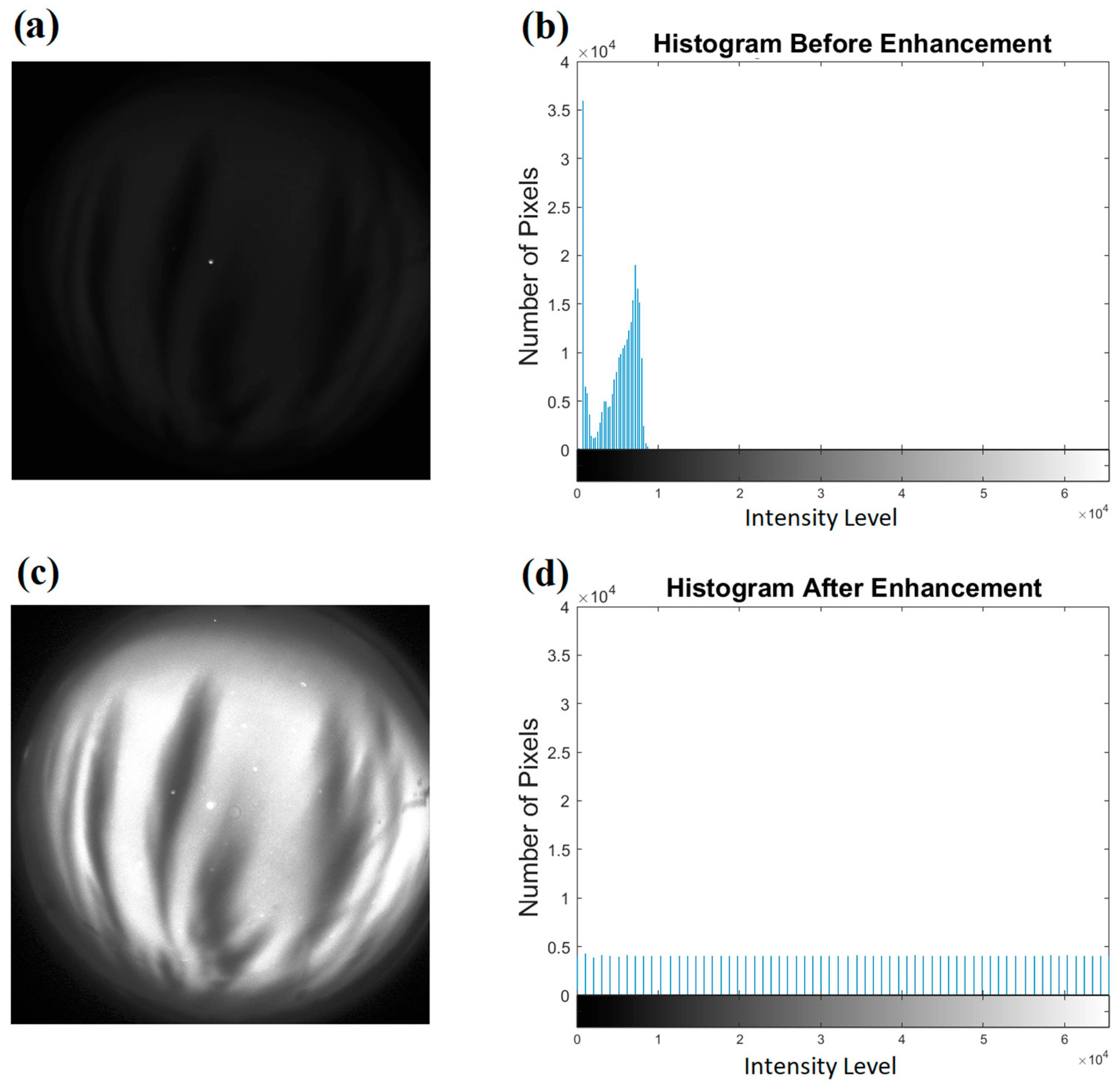
2.1. Images Pre-Processing

Before building the dataset, the images went through a pre-processing stage. To enhance the visual information within the images to choose the proper images for each dataset, a histogram equalization [44] was performed according to the following process:

First, identify the histogram of the image using Equation (4). The image contains pixel intensities ranging from $r=0$, representing the darkest intensity, to $r=L-1$, representing the brightest intensity, and $L$ is the total number of the possible intensity levels:

$$h\left(r_k\right)={\displaystyle \frac{n_k}{n}}$$

(4)

where $k$ is referring to the intensity level, $n_k$is the number of pixels with intensity $r_k$, and $n$ is the total number of the image’s pixels.

Then, compute the Cumulative Distribution Function (CDF) through the following equation:

$$c\left(r_k\right)=\sum _{j=0}^{k}h\left(r_j\right)$$

(5)

Finally, use the transformation function to obtain the new pixel intensities through Equation (6):

$$s_k=c\left(r_k\right)\times (L-1)$$

(6)

where $s_k$ is the new pixel intensity level and $L$ is the total number of the possible intensity levels.

Figure 1a shows a sample raw image captured at the Bom Jesus da Lapa (BJL) observatory (Geo 13.3 °S, 43.5 °W) on 8 October 2021 at 00:02:25. The histogram corresponding to the image is shown in Figure 1b, where most of the pixel intensity levels are concentrated on the darker side of the histogram. In contrast, Figure 1c displays the same image after enhancement, revealing its features using the mentioned method. The histogram corresponding to the enhanced image is shown in Figure 1d, where the pixel intensities are distributed across the full possible range, enhancing visualization.

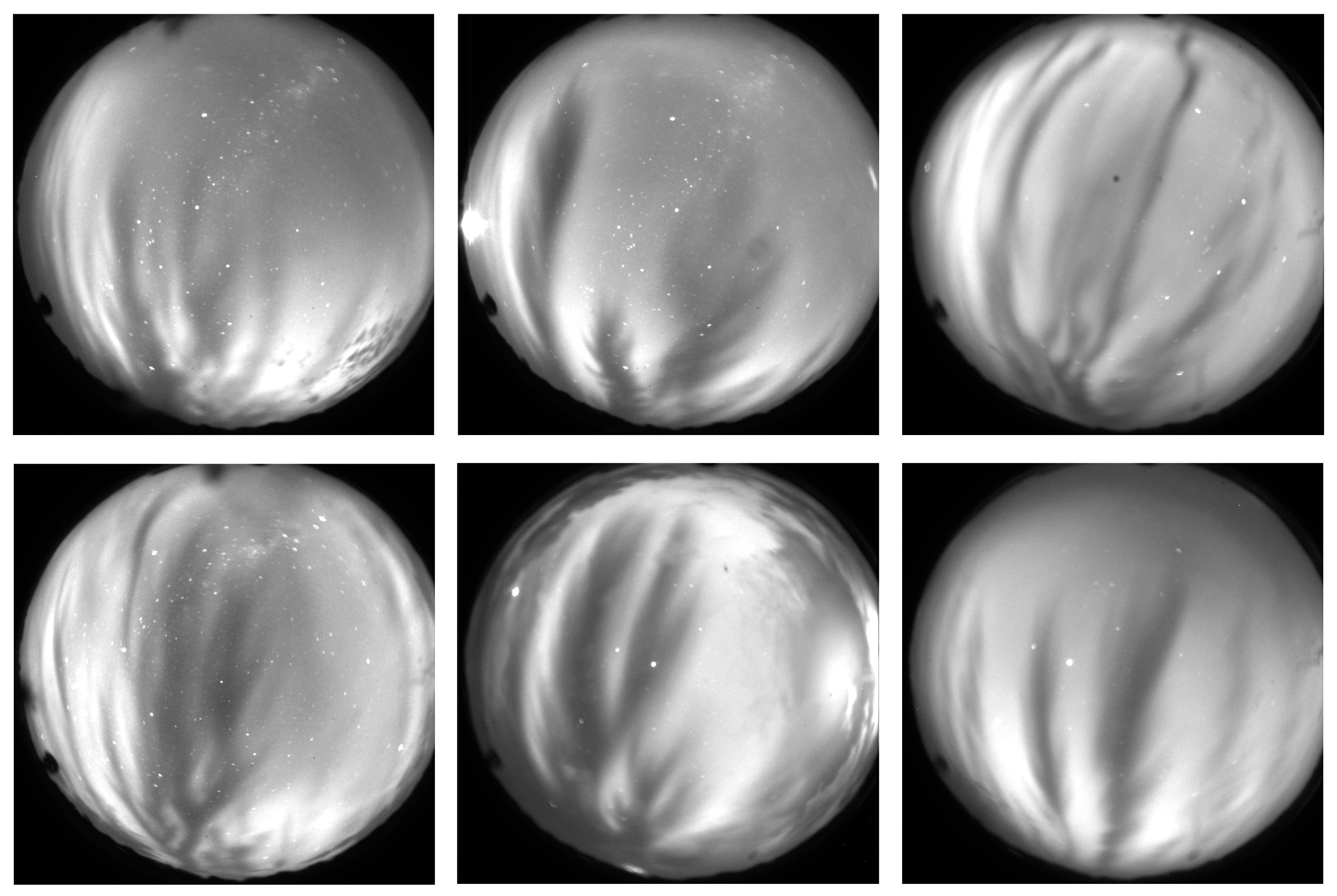
2.2. Dataset Preparation

The ASI dataset used in this study was collected from the BJL (Geo 13.3°S, 43.5°W) and São João do Cariri observatory (CA) (Geo 7.4°S, 36.6°W). These stations are part of the Embrace/INPE network. The data collection period spans from January 2020 to January 2022. The dataset considered seasonal and local time variations. The set comprises 2458 ASI raw images, manually classified based on their corresponding pre-enhanced images. The dataset was divided into two categories. The first category is the ‘Event’ Class, which includes images containing visible plasma bubbles characterized by distinct depletions in brightness and elongated structures along Earth’s magnetic field lines, originating from the magnetic equator and extending toward the poles, as shown in Figure 2. The second category is the ‘Empty’ Class, which consists of images without any apparent plasma bubble structures. The first category contains 1242 images while the second contains 1216 images. The dataset was then divided randomly into two subsets: training set and test set, following the split of 80% training set (1967 images) and 20% test set (491 images). It is crucial to ensure enough samples for training while avoiding too few samples for testing.

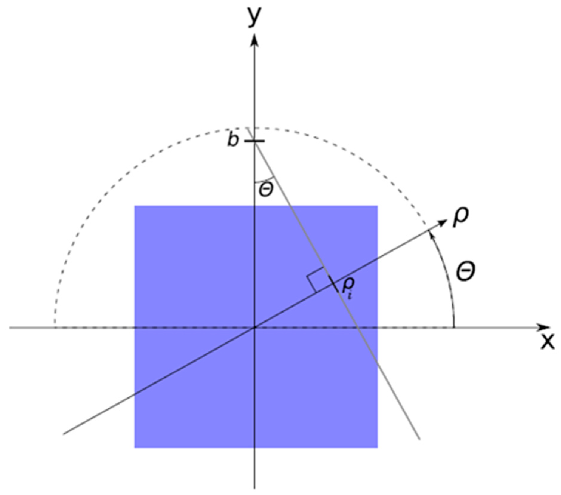
2.3. Radon Transform

To facilitate the detection process, the chosen datasets have been transformed using the Radon transform. The Radon transform is a mathematical technique that involves transforming a two-dimensional function (image) $f(x,y)$ into a set of its projections, where x = 0 and y = 0 lay at the center of the image. The resulting projection is the sum of the pixel intensities in each direction, essentially forming an integral line taken along various directions. The result is a new image $R\left(\rho ,\theta \right)$ [45].

$$\rho =xcos \theta +ysin \theta$$

(7)

where $\rho$ is the distance of the line from the origin and $\theta$ is the angle between the perpendicular to the line and the x-axis. The transformation process is depicted in Figure 3.

Radon transform is defined mathematically using the following equations:

$$R\left(\rho ,\theta \right)={\int }_{-\mathrm{\infty }}^{\mathrm{\infty }}{\int }_{-\mathrm{\infty }}^{\mathrm{\infty }}f\left(x,y\right)\delta \left(\rho -xcos \theta -ysin \theta \right)dxdy$$

(8)

where $\delta$ is the Dirac delta function.

Figure 4 illustrates examples of original images $f\left(x,y\right)$ of size 512 × 512 pixels and their corresponding Radon-transformed images $R\left(\rho ,\theta \right)$ of size 729 × 180 pixels for samples from each class. Figure 4a shows the original image of the “Empty” class, while Figure 4b presents its Radon-transformed counterpart. Similarly, Figure 4c displays the original image of the “Event” class and Figure 4d depicts its transformed version.

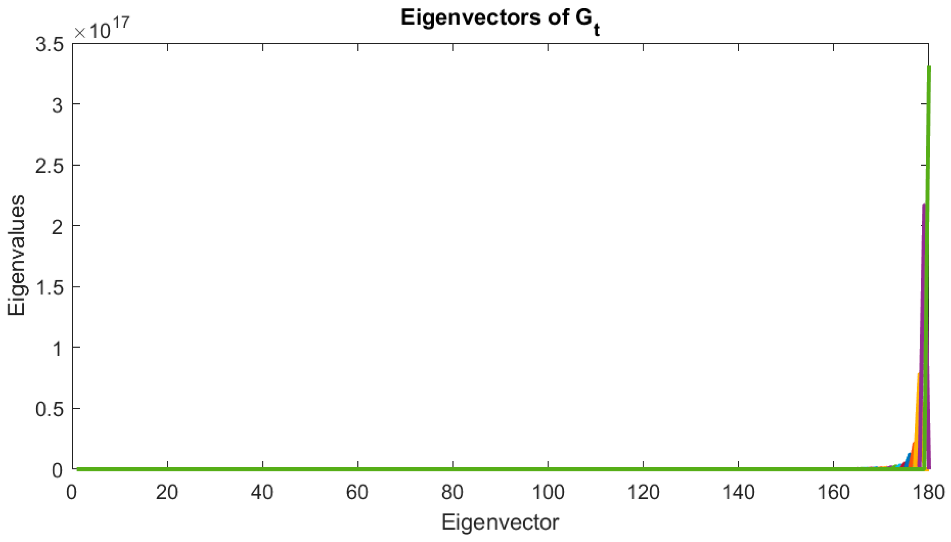
2.4. Two-Dimensional Principal Component Analysis

The main concept of Two-Dimensional Principal Component Analysis (2DPCA) is to obtain an m-dimensional projected vector that contains the image features through the following linear transformation:

$$\mathbf{Y}=\mathbf{A}\mathbf{X}$$

(9)

where $\mathbf{A}$ is an image of the dimensions $m\times n$, $\mathbf{X}$ is a unitary column vector, and $\mathbf{Y}$ is the projected feature vector of image $\mathbf{A}$ [33]. In the case of the raw airglow images (Figure 4c) at BJL, the size of $\mathbf{A}$ is 512 × 512. Meanwhile, for the Radon-transformed images (Figure 4d), the size of $\mathbf{A}$ is 729 × 180.

It starts with computing a non-negative $n\times n$ definite matrix called the image covariance matrix ${\mathbf{G}}_{\mathrm{t}}$ using the training dataset:

$${\mathbf{G}}_{\mathrm{t}}={\displaystyle \frac{1}{M}}\sum _{j=1}^M{\left({\mathbf{A}}_j-\overline{\mathbf{A}}\right)}^T\left({\mathbf{A}}_j-\overline{\mathbf{A}}\right)$$

(10)

where $M$ is the number of the training images samples, ${\mathbf{A}}_j$ is the $j$th image of the training dataset, and $\overline{\mathbf{A}}$ is the average image of all training set images.

To determine a good projection vector $\mathbf{X}$, we measure its discriminatory power using the total scatter of the projected samples. The trace of the covariance matrix of the projected feature vectors characterizes this total scatter. A higher trace indicates a better projection vector as it implies greater variance and better discrimination between projected samples.

The optimal projection axis ${\mathbf{X}}_{opt}$ is the unitary vector that maximizes the generalized total scatter of the projected samples, which corresponds to the eigenvector of the covariance matrix ${\mathbf{G}}_{\mathrm{t}}$ with the largest eigenvalue [46]. However, typically, more than one optimal projection axis is needed. A set of projection axes ${\mathbf{X}}_1,\dots ,{\mathbf{X}}_d$ is selected. These optimal projection axes are the orthonormal eigenvectors of ${\mathbf{G}}_{\mathrm{t}}$ corresponding to the largest $d$ eigenvalues. This process ensures that the most important image feature information is contained within the smallest amount of data. Figure 5 shows the graphical representation of the 2DPCA implementation.

In this study, $d$ was set to a dynamic range to determine the best accuracy based on models trained with different numbers of principal components. However, the last ten eigenvectors accounted for most of the image features, as illustrated in Figure 6.

The feature extraction of image $\mathbf{A}$ is conducted using the optimal projection vectors ${\mathbf{X}}_1,\dots ,{\mathbf{X}}_d$:

$${\mathbf{Y}}_k=\mathbf{A}{\mathbf{X}}_k,k=\mathrm{1,2},\dots ,d.$$

(11)

where ${\mathbf{Y}}_k$ refers to the $k$th vector of the projected feature vectors ${\mathbf{Y}}_1,\dots ,{\mathbf{Y}}_d$, which are called the principal component vectors of Image $\mathbf{A}$.

The feature matrices of the training dataset images are saved as the database for classification purposes. A 2DPCA transformation is performed on each image of the testing dataset. Classification is then conducted by finding the nearest neighbor classifier through calculating the distance between the testing image feature matrix and every matrix in the database:

$${\mathrm{d}(\mathbf{B}}_i,{\mathbf{B}}_j)=\sum _{k=1}^d{‖{{\mathbf{Y}}_k}^{\left(i\right)}-{{\mathbf{Y}}_k}^{\left(j\right)}‖}_2$$

(12)

where ${\mathbf{B}}_i,{\mathbf{B}}_j$ are two arbitrary feature matrices testing and training images and ${‖{{\mathbf{Y}}_k}^{\left(i\right)}-{{\mathbf{Y}}_k}^{\left(j\right)}‖}_2$ is the Euclidean distance between two principal component vectors ${{\mathbf{Y}}_k}^{\left(i\right)}$ and ${{\mathbf{Y}}_k}^{\left(j\right)}$.

Assume that the training samples are ${\mathbf{B}}_1,{\mathbf{B}}_{2,}\dots ,{\mathbf{B}}_M$ where $M$ is the total number of training samples. Each sample is assigned a specific class ${\omega }_k$. For the test sample $\mathbf{B}$, if $d \left(\mathbf{B},{\mathbf{B}}_t\right)=\mathit{min}\left(\mathbf{B},{\mathbf{B}}_j\right)$ and ${\mathbf{B}}_t\in {\omega }_k$, then the result will be $\mathbf{B}\in {\omega }_k.$ In this study, we used a collective decision based on the first three $\mathit{min}\left(\mathbf{B},{\mathbf{B}}_j\right)$, as it helped to enhance classification accuracy.

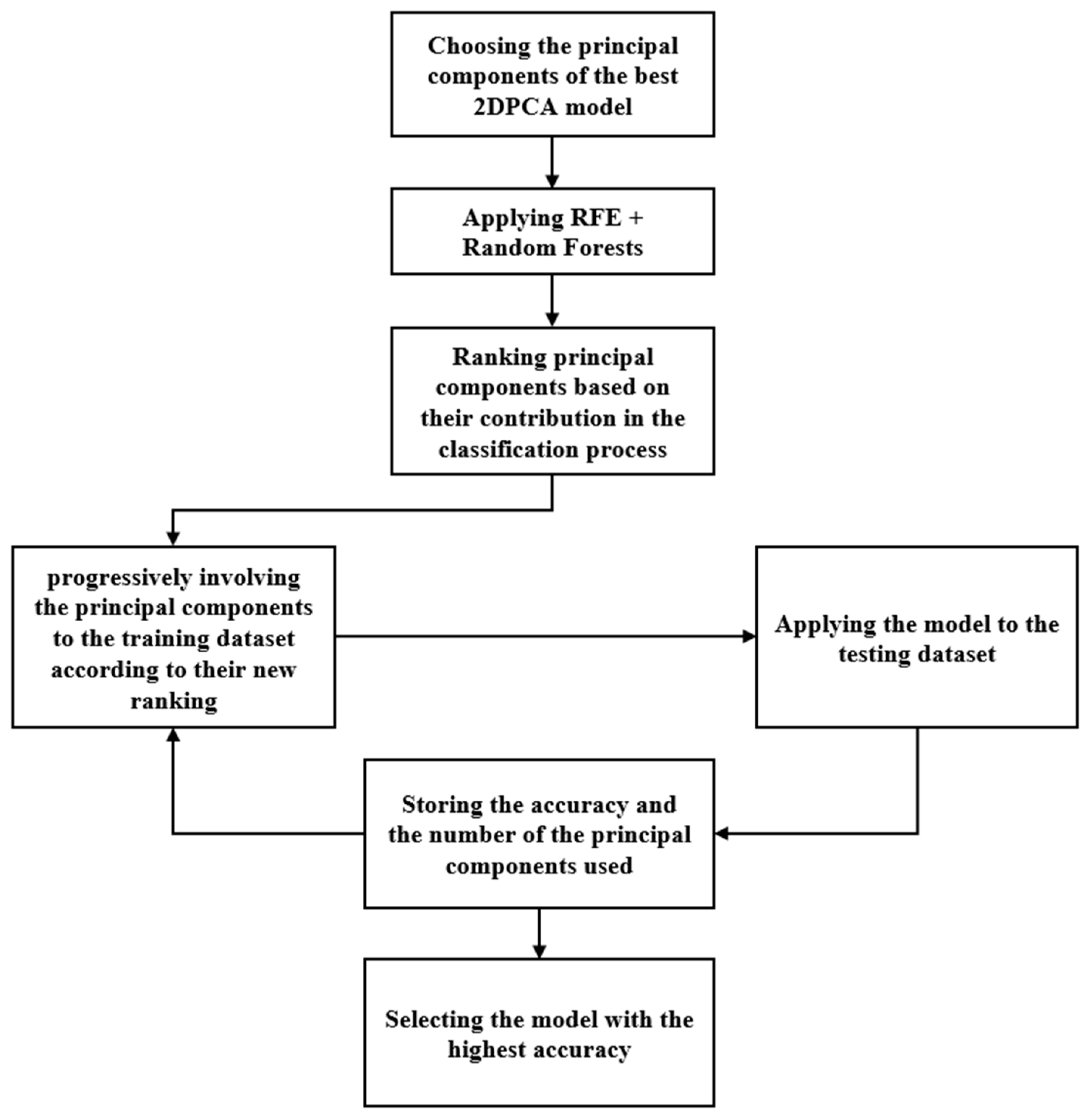
2.5. Explainable AI (XAI) Model

The output 2DPCA matrix of each image in the dataset was flattened to be introduced into a vector. This vector represented the features derived from the 2DPCA and a last column was added to represent the class. The class column was labeled either 0 or 1, where the first refers to the Empty class and the latter refers to the Event class. These vectors were combined into a single matrix where each row corresponded to an image and the last column denoted the associated class label. This matrix is used as an input to a machine learning model that performs Recursive Feature Elimination (RFE) in conjunction with Random Forest to determine the contribution of each principal component in the classification process.

2.5.1. Random Forest

Random Forest [48] is a widely used ensemble learning method in machine learning, particularly effective for classification and regression tasks. It constructs a collection of tree-structured classifiers, where each tree is grown based on a random vector ${\mathsf{\Theta }}_k$ that is sampled independently and with the same distribution for all trees in the forest. The model aggregates predictions from all trees to enhance accuracy and robustness. For classification, Random Forests determine the predicted class through majority voting and, for regression, they compute the average of the tree outputs. The principles of Random Forests are based on determining the margin function, the strength of individual classifiers, and the correlation between trees, as well as their impact on generalization error. These foundational principles enable Random Forests to achieve high accuracy, avoid overfitting, and provide estimates of variable importance, making them a robust and versatile machine learning method.

The margin function, which quantifies the confidence of the classification, is defined as:

$$mr\left(X,Y\right)=P_{\mathsf{\Theta }}\left(h\left(X,\mathsf{\Theta }\right)=Y\right)-{max}_{j\ne Y}{P}_{\mathsf{\Theta }}(h\left(X,\mathsf{\Theta }\right)=j)$$

(13)

where $h \left(X,\mathsf{\Theta }\right)$ is the prediction of a tree, $P_{\mathsf{\Theta }}$ is the probability measure over the random vectors $\mathsf{\Theta }$, $X$ is the input, and $Y$ is the true class label. A larger margin indicates higher confidence in the classification decision.

The strength of the forest is the expected value of the margin function:

$$s=E_{X,Y}\left[mr\left(X,Y\right)\right]$$

(14)

where $s$ measures the average accuracy of the individual trees in the forest.

The generalization error, which represents the probability of misclassification, is shown to have the upper bound:

$$P{E}^{*}\le {\displaystyle \frac{\overline{\rho }(1-s^2)}{s^2}}$$

(15)

where $\overline{\rho }$ is the average correlation between the classifiers in the forest. This equation highlights the balance between the individual trees’ strength and their correlation, underscoring that the effectiveness of Random Forests relies on achieving high tree strength while maintaining low correlation between them.

2.5.2. Recursive Feature Elimination (RFE)

RFE is a feature selection method, particularly suitable for small sample classification problems [49]. It was initially applied to microarray-based cancer classification, where training samples are fewer than 100, while the number of features can reach several thousand, proving to be a powerful technique for feature selection. RFE ranks the features by iteratively fitting a model (logistic regression in our case) and removing the least important features at each step until the desired number of features is reached. Then, it gives the ranking for all original features.

2.5.3. Algorithm Breakdown

The dataset was divided into training and testing subsets. The process begins by loading the training dataset and applying 2DPCA to reduce the high-dimensional image data into a set of principal components, retaining the most significant features in a compact form. The accuracy of 2DPCA is evaluated by testing a dynamic range of principal components with the highest eigenvalues to identify the group responsible for the highest accuracy. The trained data corresponding to the principal components with the highest accuracy are then flattened and fed into RFE in conjunction with Random Forests. The Random Forest classifier is used as the base estimator for RFE. RFE iteratively eliminates the least important features based on Random Forest’s feature importance metrics, progressively refining the feature set to the desired number of principal components. For each iteration, feature importance is aggregated across the components and their overall contribution to the model’s decision making is calculated. The final output includes ranked feature importance scores and visualizations showing feature contributions and their percentage impact on the classification. These steps ensure the model not only achieves high accuracy but also provides clear insights into which principal components drive its predictions, aligning with the principles of XAI. Finally, the top three contributing components are selected to create the final trained model, achieving the highest accuracy with the smallest possible size. The algorithm flowchart is shown in Figure 7.

2.6. Evaluation Parameters

The evaluation parameters for the results of the predictions of the models are defined as follows:

• Accuracy measures the overall performance of the model by computing the ratio of correct predictions to the total number of tested samples:

  $$\mathit{Accuracy}={\displaystyle \frac{\mathit{True}\mathit{Positive}+\mathit{True}\mathit{Negative}}{\mathit{Total}\mathit{number}\mathit{of}\mathit{predictions}}}$$

  (16)

  where $\mathit{True}\mathit{Positive}$ is the number of images in which the model correctly detected an EPB when it was actually present. $\mathit{True}\mathit{Negative}$ is the number of images in which the model correctly classified an image as not containing an EPB when it was absent;
• Precision evaluates the accuracy of positive predictions by calculating the proportion of correctly detected EPBs ($\mathit{True}\mathit{Positives}$) out of all assumed detected EPBs:

  $$\mathit{Precision}={\displaystyle \frac{\mathit{True}\mathit{Positive}}{\mathit{True}\mathit{Positive}+\mathit{False}\mathit{Positive}}}$$

  (17)

  where $\mathit{False}\mathit{Positive}$ is the number of images in which the model incorrectly detected an EPB when none were present;
• Recall assesses the model’s ability to identify all positive instances by calculating the ratio of True Positives to the sum of $\mathit{True}\mathit{Positives}$ and $\mathit{False}\mathit{Negatives}$:

  $$\mathit{Recall}={\displaystyle \frac{\mathit{True}\mathit{Positive}}{\mathit{True}\mathit{Positive}+\mathit{False}\mathit{Positive}}}$$

  (18)

  where $\mathit{False}\mathit{Negatives}$ is the number of images in which the model failed to detect an EPB when one was actually present (a missed detection);
• F1-score provides a balanced measure of the model’s performance by combining both precision and recall into a single metric:

  $$F1 \mathit{score}=2\times {\displaystyle \frac{\mathit{Precision}\times \mathit{Sensitvity}}{\mathit{Precision}+\mathit{Sensitvity}}}$$

  (19)

3. Results and Discussion

The standard proposed 2DPCA model without applying Radon transform was trained multiple times using the training dataset, each time using a different number of the highest principal components, which corresponded to varying cuts of the total eigenvalues within the dataset. This cut was set to be equal to 95% or higher. The model was then tested using the testing dataset, which was selected randomly and kept consistent across all tests. The testing results showed unexpected fluctuations in detection accuracy, unlike the expectations, as increasing the percentage of eigenvalues was assumed to correlate with a higher number of trained features (according to Yang and Yang) [46]. This may be due to the dataset’s dependency as the dataset consists of airglow images taken under different atmospheric and geomagnetic conditions. Variations in cloud cover, background noise, and observational conditions may introduce inconsistencies that affect the model’s performance across different test sets.

Table 1. Detection accuracy based on 2DPCA without using Radon transform.

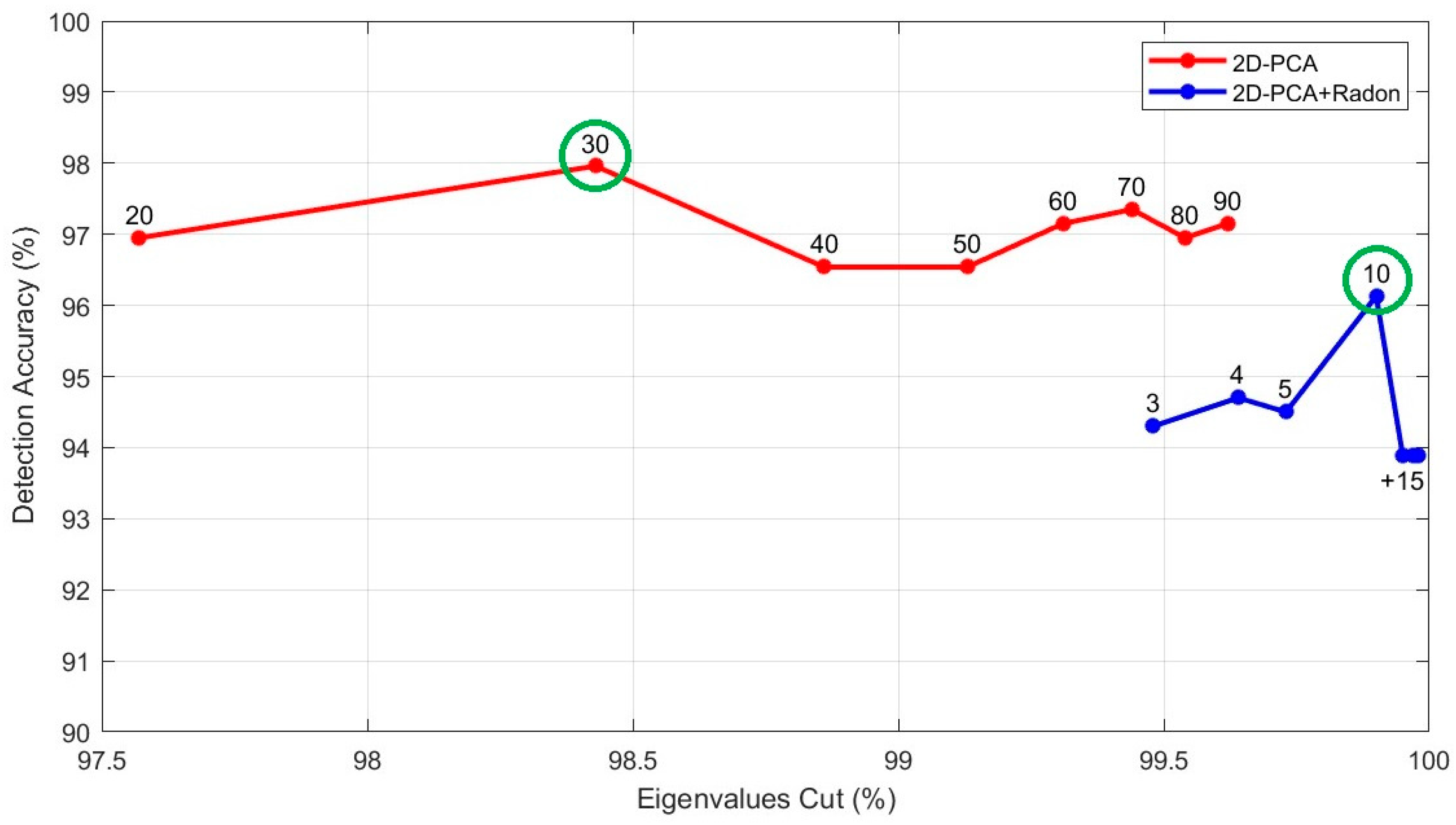
Number of Principal Components	Eigenvalues Cut (%)	Accuracy (%)	Elapsed Time (s)
20	97.57	96.95	301.692
30	98.43	97.96	301.748
40	98.86	96.54	301.705
50	99.13	96.54	301.896
60	99.31	97.15	301.766
70	99.44	97.35	301.918
80	99.54	96.95	301.916
90	99.62	97.15	301.879

shows the number of the selected eigenvectors with the highest eigenvalues, their percentages to the total of eigenvalues, the detection accuracy, and the training time consumed using the training dataset, which contains 1967 images.

The 2DPCA model was then trained again using the same criteria after applying Radon transform. Re-processing the images using Radon transform helped to change the image resolution from 512 × 512 pixels to 729 × 180, which resulted in getting a smaller covariance matrix with only 180 eigenvectors in total instead of 512. This resulted in getting a smaller number of eigenvectors that correspond to the same cut of eigenvalues in the previous test, hence noticeably reducing the training time and the model size. However, applying Radon transform to raw images caused a decrease in the detection accuracy.

Table 2. Detection accuracy based on 2DPCA using Radon transform.

Number of Principal Components	Eigenvalues Cut (%)	Accuracy (%)	Elapsed Time (s)
3	99.48	94.30	130.660
4	99.64	94.70	130.678
5	99.73	94.50	130.673
10	99.90	96.13	130.683
15	99.95	93.89	130.793
20	99.97	93.89	130.751
25	99.98	93.89	130.873

shows the percentage of the contributed features, the training time, and the accuracy for different selected numbers of the highest eigenvectors.

Figure 8 provides a visual comparison of the results from Table 1 and Table 2. The x-axis represents the cut-off percentages of the eigenvalues of principal components that were used to train the model to the total eigenvalue sum while the y-axis indicates the detection accuracy corresponding to each percentage. Additionally, the number of principle components used to train the 2DPCA model is written above each point. The plot indicates that all trained models using raw images achieve better accuracy than those using Radon-transformed images. Furthermore, the models yielding the highest accuracy for each training type were as follows: for raw images, the model utilizing the top thirty principal components achieved a detection accuracy of 97.96% while, for Radon-transformed images, the model using the top ten principal components achieved a detection accuracy of 96.1%. These models are marked with green circles.

RFE, in conjunction with Random Forest, was then applied to the models responsible for the highest detection accuracy at each case to determine the contribution of each principal component in the image classification process. Figure 9a shows the eigenvalues of the principal components. Meanwhile, Figure 9b shows the percentage of contribution of each principal component in determining the class of the testing images based on RFE and Random Forest. The comparison between both panels reveals that principal components with the highest eigenvalues do not necessarily contribute the most to the classification process. For instance, the 30th principal component, despite having the smallest eigenvalue, was the highest contributor to the classification process. Similarly, Figure 9c,d illustrate the eigenvalues of the principal components for the model utilizing Radon-transformed images and their corresponding percentage contributions to the classification process. Although the tenth and ninth eigenvectors have the smallest eigenvalues, their principal components ranked as the first and third highest contributors in the classification process, respectively.

The XAI model ranks the principal components based on their contributions. It then utilizes 2DPCA, progressively incorporating the principal components into the training process according to their new ranking, and then applies it to the testing subset. Next, it stores the number of principal components used and the detection accuracy of the model. Finally, it selects the model that achieves the highest detection accuracy while maintaining the smallest possible size. This process is illustrated in Figure 10. The new models were based on the top thirteen and top three principal component contributors for the raw and Radon-transformed models, respectively. These models achieved an increase in detection accuracy of 0.21% for the raw image-based model, reaching 98.17%, and an increase of 1.22% for the Radon-transformed image-based model, reaching 97.35%. Furthermore, they had significantly smaller sizes compared to the original models, with size reductions of 56.6% and 70% for the raw and Radon-transformed models, respectively.

The proposed model was compared with other deep learning baseline models, including ResNet18, Inception-V3, VGG16, and VGG19 [50,51], to evaluate its performance. These CNN models were trained using the aforementioned split database, without applying any transfer learning, while preserving their original architecture. To ensure a fair comparison, all models were trained in a similar environment. Moreover, the same hyperparameters were applied across all models, with a batch size of 16. The epoch limit was set at 10 to reduce training time with the possibility of retrieving the epoch with the best validation accuracy and lowest training loss. The original training dataset was split into training and validation subsets, with 80% allocated for training and 20% for validation. All datasets were kept consistent across all models. The performance of each model was assessed using the evaluation parameters mentioned in Section 2. The results of these evaluation parameters for all models are presented in

Table 3. Model evaluation results for the EPB detection of different deep learning models, the proposed 2DPCA, and XAI models.

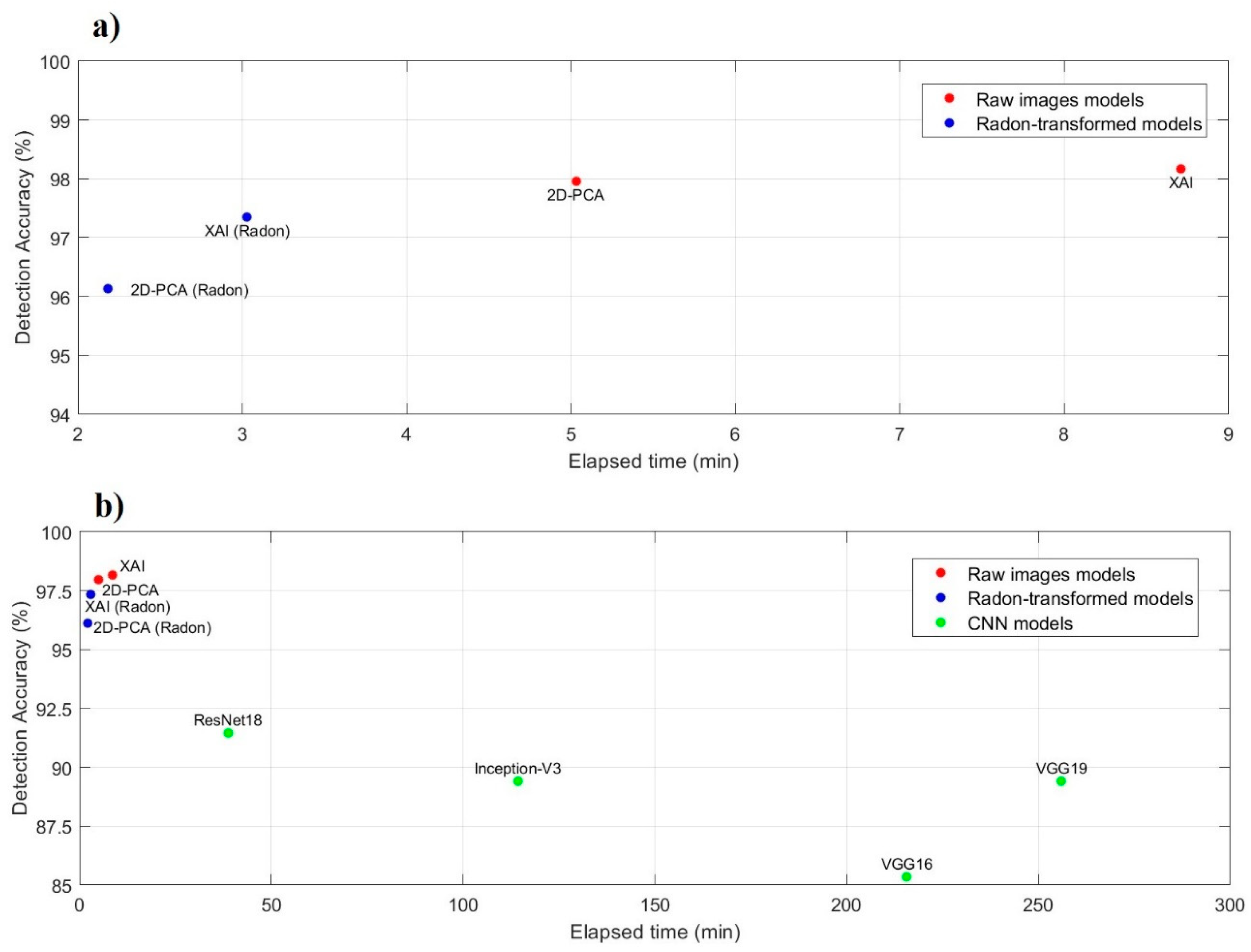
Model	Accuracy (%)	Precision (%)	Sensitivity (%)	F1-Score (%)	Elapsed Time (min)
ResNet18	91.45	92.76	91.36	92.05	38.72
Inception-V3	89.41	90.78	89.32	90.04	114.30
VGG16	85.34	88.35	85.19	86.74	215.70
VGG19	89.41	90.32	89.33	89.83	255.96
2DPCA	97.96	98.03	97.95	97.99	5.03
2DPCA (Radon)	96.13	96.37	96.17	96.27	2.18
XAI	98.17	98.18	98.16	98.17	8.71
XAI (Radon)	97.35	97.43	97.38	97.40	3.03

.

The results from Table 3 are visualized in Figure 11. Figure 11a highlights the differences among the proposed models, illustrating the relationship between detection accuracy and elapsed training time. Figure 11b presents the same relationship, with the addition of deep learning CNN models for comparison. The figure shows that the best detection accuracy was achieved by the XAI model based on the raw data, achieving 98.17% and overpassing all other proposed models and CNN deep learning models, while the lowest accuracy was obtained by VGG16. However, the XAI model using Radon-transformed images demonstrated the best performance in terms of a balance between accuracy and elapsed time. While it achieved the second-best detection accuracy with only a 0.82% difference from the top model, it required significantly less time, taking just 35% of the time consumed by the first model to achieve the highest accuracy. Furthermore, the proposed method of using 2DPCA required significantly less training time in the same environment compared to the deep learning baseline models. While the incorporation of XAI slightly increased the training time compared to 2DPCA, it contributed to an improvement in detection accuracy and a reduction in the trained model size. Using the proposed XAI model with a small elapsed time enables the creation of compact and fast-trained detection models that consume low computational power while providing high accuracy. Such models are suitable for integration with real-time detection techniques and for deployment in low-cost systems. However, the model may be sensitive to partially cloudy sky conditions, where a single image contains both plasma bubbles and clouds. This can lead to misclassification or failure to recognize actual plasma bubbles due to obstructions in real-time detection. Despite this challenge, equatorial plasma bubbles remain in the field of view longer than clouds. This allows for a more reliable approach based on collective decisions from multiple ASI images, reducing false detections and improving accuracy.

4. Conclusions

In this study, a low-computational-cost XAI model was developed for the automatic detection of equatorial plasma bubbles in ASI data. This model was based on using 2DPCA with RFE, in conjunction with a Random Forest machine learning model. A dataset of 2458 ASI images was collected and classified manually into two classes: “Empty” class when the image does not contain a plasma bubble and “Event” class when a plasma bubble appears in the image. This dataset was split into two subsets: the training subset (80%) and the testing subset (20%). These subsets remained constant among all the classification tests. The first training instance was conducted using only 2DPCA applied to the raw images, achieving a detection accuracy of 97.96%. Applying Radon transform in the further testing helped in decreasing the computational time and the size of the trained model by almost 65% but reduced the detection accuracy to 96.1%.

The XAI model was then utilized by using the eigenvectors from the models with the highest detection accuracy to determine the actual contribution of each principal component in the classification process. These principal components were then ranked based on the contribution percentage using RFE in conjunction with Random Forest. Based on their updated ranking, the principal components were gradually incorporated into the 2DPCA training process to develop a model that maximizes detection accuracy while minimizing its size. Although the implementation of the XAI model slightly increased the processing time compared to 2DPCA, it improved detection accuracy for the raw image-based model by 0.21%, achieving 98.17%, and caused an increase of 1.22% for the Radon-transformed image-based model, reaching 97.35%. It reduced the size of the trained detection models compared to the standard 2DPCA, with a reduction of 56.6% for the raw image-based model and 70% for the Radon-transformed model. Additionally, the comparison with the deep learning CNN models showed the superiority of the proposed models in the detection accuracy within the raw ASI images and for the training time. The highest detection accuracy among the CNN baseline models was achieved by ResNet18 at 91.45%, placing it 4.68% to 6.72% behind the proposed models. Additionally, ResNet18 was the fastest deep learning model, requiring 38.72 min to train over 10 epochs, whereas the proposed models required only 2.18 to 8.71 min to be trained in the same environment. The proposed models are well-suited for integration with real-time detection techniques and deployment in low-cost systems. Although the model may be sensitive to partially cloudy conditions, which can lead to potential misclassification, EPBs remain in the field of view of the ASI for a long time. This can enhance accuracy through the collective decision making of multiple ASI images, reducing false detections and improving overall performance.

References

- Hysell, D.L.; Woodman, R.F. Imaging coherent backscatter radar observations of topside equatorial spread F. Radio Sci. 1997, 32, 2309–2320. [Google Scholar] [CrossRef]
- Kelley, M.C. The Earth’s Ionosphere; Academic Press: San Diego, CA, USA, 1989. [Google Scholar]
- Basu, S.; Kudeki, E.; Basu, S.; Valladares, C.E.; Weber, E.J.; Zengingonul, H.P.; Espinoza, J. Scintillations, plasma drift, and neutral winds in the equatorial ionosphere after sunset. J. Geophys. Res. 1996, 101, 26795–26809. [Google Scholar] [CrossRef]
- Kintner, P.M.; Kil, H.; Ledvina, B.M.; Paula, E.D. Fading timescales associated with GPS signals and potential consequences. Radio Sci. 2001, 36, 731–743. [Google Scholar] [CrossRef]
- Straus, P.R.; Anderson, P.C.; Danaher, J.E. GPS occultation sensor observations of ionospheric scintillation. Geophys. Res. Lett. 2003, 30, 1436. [Google Scholar] [CrossRef]
- Park, J.; Noja, M.; Stolle, C.; Luhr, H. The ionospheric bubble index deduced from magnetic field and plasma observations onboard swarm. Earth Planets Space 2013, 65, 1333–1344. [Google Scholar] [CrossRef]
- Weber, E.J.; Brinton, H.C.; Buchau, J.; Moore, J.G. Coordinated airborne and satellite measurements of equatorial plasma depletions. J. Geophys. Res. 1982, 87, 10503–10513. [Google Scholar] [CrossRef]
- Tinsley, B.A.; Rohrbaugh, R.P.; Hanson, W.B.; Broadfoot, A.L. Images of transequatorial F region bubbles in 630- and 777-nm emissions compared with satellite measurements. J. Geophys. Res. 1997, 102, 2057–2077. [Google Scholar] [CrossRef]
- Su, S.-Y.; Yeh, H.C.; Heelis, R.A. ROCSAT-1 ionospheric plasma and electrodynamics instrument observations of equatorial spread F: An early transitional scale result. J. Geophys. Res. 2001, 106, 29153–29159. [Google Scholar] [CrossRef]
- Kelley, M.C.; Makela, J.J.; Ledvina, B.M.; Kintner, P.M. Observations of equatorial spread-F from Haleakala, Hawaii. Geophys. Res. Lett. 2002, 29, 2003. [Google Scholar] [CrossRef]
- Makela, J.J.; Miller, E.S. Optical observations of the growth and day-to-day variability of equatorial plasma bubbles. J. Geophys. Res. Space Phys. 2008, 113, 1–7. [Google Scholar] [CrossRef]
- Sobral, J.H.; Takahashi, H.; Abdu, M.A.; Muralikrishna, P.; Sahai, Y.; Zamlutti, C.J.; De Paura, R.E.; Batista, P.P. Determination of the quenching rate of the O(1D) by O(3P) from rocket-borne optical (630 nm) and electron density data. J. Geophys. Res. 1993, 98, 7791–7798. [Google Scholar] [CrossRef]
- Pimenta, A.A.; Fagundes, P.R.; Bittencourt, J.A.; Sahai, Y.; Gobbi, D.; Medeiros, A.F.; Taylor, M.J.; Takahashi, H. Ionospheric plasma bubble zonal drift: A methodology using OI 630 nm all-sky imaging systems. Adv. Space Res. 2001, 27, 1219–1224. [Google Scholar] [CrossRef]
- Weber, E.J.; Buchau, J.; Eather, R.H.; Mende, S.B. North-south aligned equatorial depletions. J. Geophys. Res. 1978, 83, 712–716. [Google Scholar] [CrossRef]
- Mendillo, M.; Baumgardner, J.; Sultan, P.J. Airglow characteristics of equatorial plasma depletions. J. Geophys. Res. 1982, 87, 7641–7652. [Google Scholar] [CrossRef]
- Taylor, M.J.; Eccles, J.V.; Labelle, J.; Sobral, J.H.A. High-resolution OI (630 nm) image measurements of F-region depletion drifts during the Guara campaign. Geophys. Res. Lett. 1997, 24, 1699–1702. [Google Scholar] [CrossRef]
- Fagundes, P.R.; Sahai, Y.; Batista, I.S.; Abdu, M.A.; Bittencourt, J.A.; Takahashi, H. Observations of day-to-day variability in precursor signatures to equatorial F-region plasma depletions. Ann. Geophys. 1999, 17, 1053–1063. [Google Scholar] [CrossRef]
- Makela, J.J.; Ledvina, B.M.; Kelley, M.C.; Kintner, P.M. Analysis of the seasonal variations of equatorial plasma bubble occurrence observed from Haleakala. Hawaii. Ann. Geophys. 2004, 22, 3109–3121. [Google Scholar] [CrossRef]
- Mendillo, M.; Zesta, E.; Shodhan, S.; Doe, R.; Sahai, Y.; Baumgardner, J. Observations and modeling of the coupled latitude-altitude patterns of equatorial plasma depletions. J. Geophys. Res. 2005, 110, A09303. [Google Scholar] [CrossRef]
- Rajesh, P.K.; Liu, J.Y.; Sinha, H.S.S.; Banerjee, S.B.; Misra, R.N.; Dutt, N.; Dadhania, M.B. Observations of plasma depletions in 557.7-nm images over Kavalur. J. Geophys. Res. Space Phys. 2007, 112, A07307. [Google Scholar] [CrossRef]
- Liu, J.Y.; Tsai, H.F.; Jung, T.K. Airglow observations over the equatorial ionization anomaly zone in Taiwan. Ann. Geophys. 2011, 29, 749–757. [Google Scholar] [CrossRef]
- Shiokawa, K.; Otsuka, Y.; Lynn, K.J.; Wilkinson, P.; Tsugawa, T. Airglow-imaging observation of plasma bubble disappearance at geomagnetically conjugate points. Earth Planet Space 2015, 67, 43. [Google Scholar] [CrossRef]
- Fukushima, D.; Shiokawa, K.; Otsuka, Y.; Nishioka, M.; Kubota, M.; Tsugawa, T.; Nagatsuma, T.; Komonjinda, S.; Yatini, C.Y. Geomagnetically conjugate observation of plasma bubbles and thermospheric neutral winds at low latitudes. J. Geophys. Res. Space Phys. 2015, 120, 2222–2231. [Google Scholar] [CrossRef]
- Okoh, D.; Rabiu, B.; Shiokawa, K.; Otsuka, Y.; Segun, B.; Falayi, E.; Onwuneme, S.; Kaka, R. First study on the occurrence frequency of equatorial plasma bubbles over West Africa using an all-sky airglow imager and GNSS receivers. J. Geophys. Res. Space Phys. 2017, 122, 12430–12444. [Google Scholar] [CrossRef]
- Ghodpage, R.N.; Gurav, O.B.; Taori, A.; Sau, S.; Patil, P.T.; Erram, V.C.; Sripathi, S. Observation of an intriguing equatorial plasma bubble event over Indian sector. J. Geophys. Res. Space Phys. 2021, 126, e2020JA028308. [Google Scholar] [CrossRef]
- Wrasse, C.M.; Figueiredo, C.A.O.B.; Barros, D.; Takahashi, H.; Carrasco, A.J.; Vital, L.F.R.; Rezende, L.C.A.; Egito, F.; Rosa, G.M.; Sampaio, A.H.R. Interaction between equatorial plasma bubbles and a medium-scale traveling ionospheric disturbance, observed by OI 630 nm airglow imaging at Bom Jesus de Lapa, Brazil. Earth Planet. Phys. 2021, 5, 397–406. [Google Scholar] [CrossRef]
- Liu, J.-Y.; Rajesh, P.K.; Liao, Y.-A.; Chum, J.; Kan, K.-W.; Lee, I.-T. Airglow observed by a full-band imager together with multi-instruments in Taiwan during nighttime of 1 November 2021. Adv. Space Res. 2024, 73, 663–671. [Google Scholar] [CrossRef]
- Gentile, L.C.; Burke, W.J.; Rich, F.J. A global climatology for equatorial plasma bubbles in the topside ionosphere. Ann. Geophys. 2006, 24, 163–172. [Google Scholar] [CrossRef]
- Huang, C.-S.; Roddy, P.A. Effects of solar and geomagnetic activities on the zonal drift of equatorial plasma bubbles. J. Geophys. Res. Space Phys. 2016, 121, 628–637. [Google Scholar] [CrossRef]
- Wan, X.; Xiong, C.; Rodriguez-Zuluaga, J.; Kervalishvili, G.N.; Stolle, C.; Wang, H. Climatology of the occurrence rate and amplitudes of local time distinguished equatorial plasma depletions observed by Swarm satellite. J. Geophys. Res. Space Phys. 2018, 123, 3014–3026. [Google Scholar] [CrossRef]
- Adkins, V.J.; England, S.L. Automated detection and tracking of equatorial plasma bubbles utilizing Global-Scale Observations of the Limb and Disk (GOLD) 135.6 nm Data. Earth Space Sci. 2023, 10, e2023EA002935. [Google Scholar] [CrossRef]
- Chakrabarti, S.; Patgiri, D.; Rathi, R.; Dixit, G.; Krishna, M.V.S.; Sarkhel, S. Optimizing a deep learning framework for accurate detection of the Earth’s ionospheric plasma structures from all-sky airglow images. Adv. Space Res. 2024, 73, 5990–6005. [Google Scholar] [CrossRef]
- Yang, J.; Zhang, D.; Frangi, A.F.; Yang, J. Two-dimensional PCA: A new approach to appearance-based face representation and recognition. IEEE Trans. Pattern Anal. Mach. Intell. 2004, 26, 131–137. [Google Scholar] [CrossRef]
- Lin, J.-W. Ionospheric anomaly related to M=6.6, 26 August 2012, Tobelo earthquake near Indonesia: Two-dimensional principal component analysis. Acta Geod. Geophys. 2013, 48, 247–264. [Google Scholar] [CrossRef]
- Lin, J.-W. Generalized two-dimensional principal component analysis and two artificial neural network models to detect traveling ionospheric disturbances. Nat. Hazards 2022, 111, 1245–1270. [Google Scholar] [CrossRef]
- Lin, J.-W.; Chiou, J.-S.; Chao, C.-T. Detecting all possible ionospheric precursors by kernel-based two-dimensional principal component analysis. IEEE Access 2019, 7, 53650–53666. [Google Scholar] [CrossRef]
- Yu, J.; Liu, J. Two-dimensional principal component analysis-based convolutional autoencoder for wafer map defect detection. IEEE Trans. Ind. Electron. 2021, 68, 8789–8797. [Google Scholar] [CrossRef]
- Sun, Z.; Shao, Z.; Shang, Y.; Li, B.; Wu, J.; Bi, H. Randomized nonlinear two-dimensional principal component analysis network for object recognition. Mach. Vis. Appl. 2023, 34, 21. [Google Scholar] [CrossRef]
- Wang, L.; You, Z.H.; Yan, X. Using two-dimensional principal component analysis and rotation forest for prediction of protein-protein interactions. Sci. Rep. 2018, 8, 12874. [Google Scholar] [CrossRef]
- Abdelwahab, M.M.; Abdelrahman, S.A. Four layers image representation for prediction of lung cancer genetic mutations based on 2DPCA. In Proceedings of the 2017 IEEE 60th International Midwest Symposium on Circuits and Systems (MWSCAS), Boston, MA, USA, 6–9 August 2017; 2017; pp. 599–602. [Google Scholar] [CrossRef]
- Lundberg, S.M.; Lee, S.-I. A Unified Approach to Interpreting Model Predictions. Adv. Neural Inf. Process. Syst. (NeurIPS) 2017, 30. [Google Scholar] [CrossRef]
- Ribeiro, M.T.; Singh, S.; Guestrin, C. “Why should I trust you?” Explaining the predictions of any classifier. In Proceedings of the 22nd ACM SIGKDD International Conference on Knowledge Discovery and Data Mining, San Francisco, CA, USA, 13–17 August 2016; pp. 1135–1144. [Google Scholar]
- Retzlaff, C.O.; Angerschmid, A.; Saranti, A.; Schneeberger, D.; Müller, D.; Holzinger, A. Post-hoc vs ante-hoc explanations: xAI design guidelines for data scientists. Cogn. Syst. Res. 2024, 86, 101243. [Google Scholar] [CrossRef]
- Gonzalez, R.C.; Wintz, P. Digital Image Processing, 3rd ed.Addison-Wesley: Reading, MA, USA, 1997. [Google Scholar]
- Carsten, H. The Radon Transform; Aalborg University: Aalborg, Denmark, 2007; VGIS, 07gr721. [Google Scholar]
- Yang, J.; Yang, J.Y. From image vector to matrix: A straightforward image projection technique—IMPCA vs. PCA. Pattern Recognit. 2002, 35, 1997–1999. [Google Scholar] [CrossRef]
- Yin, X.; Chen, L. A Cross-Modal Image and Text Retrieval Method Based on Efficient Feature Extraction and Interactive Learning CAE. Sci. Program. 2022, 1, 7314599. [Google Scholar] [CrossRef]
- Breiman, L. Random Forests. Mach. Learn. 2001, 45, 5–32. [Google Scholar] [CrossRef]
- Guyon, I.; Weston, J.; Barnhill, S.; Vapnik, V. Gene selection for cancer classification using support vector machines. Mach. Learn. 2002, 46, 389–422. [Google Scholar] [CrossRef]
- Szegedy, C.; Vanhoucke, V.; Ioffe, S.; Shlens, J.; Wojna, Z. Rethinking the inception architecture for computer vision. In Proceedings of the IEEE Conference on Computer Vision and Pattern Recognition, Las Vegas, NV, USA, 27–30 June 2016; pp. 2818–2826. [Google Scholar]
- He, K.; Zhang, X.; Ren, S.; Sun, J. Deep residual learning for image recognition. In Proceedings of the IEEE Conference on Computer Vision and Pattern Recognition, Las Vegas, NV, USA, 27–30 June 2016; pp. 770–778. [Google Scholar]