SGRiT: Non-Negative Matrix Factorization via Subspace Graph Regularization and Riemannian-Based Trust Region Algorithm

Abstract

Non-negative Matrix Factorization (NMF) has gained popularity due to its effectiveness in clustering and feature selection tasks. It is particularly valuable for managing high-dimensional data by reducing dimensionality and providing meaningful semantic representations. However, traditional NMF methods may encounter challenges when dealing with noisy data, outliers, or when the underlying manifold structure of the data is overlooked. This paper introduces an innovative approach called SGRiT, which employs Stiefel manifold optimization to enhance the extraction of latent features. These learned features have been shown to be highly informative for clustering tasks. The method leverages a spectral decomposition criterion to obtain a low-dimensional embedding that captures the intrinsic geometric structure of the data. Additionally, this paper presents a solution for addressing the Stiefel manifold problem and utilizes a Riemannian-based trust region algorithm to optimize the loss function. The outcome of this optimization process is a new representation of the data in a transformed space, which can subsequently serve as input for the NMF algorithm. Furthermore, this paper incorporates a novel subspace graph regularization term that considers high-order geometric information and introduces a sparsity term for the factor matrices. These enhancements significantly improve the discrimination capabilities of the learning process. This paper conducts an impartial analysis of several essential NMF algorithms. To demonstrate that the proposed approach consistently outperforms other benchmark algorithms, four clustering evaluation indices are employed.

1. Introduction

Non-negative Matrix Factorization (NMF) is a clustering and dimension reduction method that approximates a matrix as a product of two nonnegative components [1]. Unlike similar techniques, NMF allows only additive combinations, leading to a parts-based representation. NMF has gained increasing attention due to its unique capability to provide interpretable results that are nonnegative, distinguishing it from other conventional subspace learning algorithms [2]. This characteristic enables NMF to effectively capture the essence of intelligent data representation [2]. While other dimension-reduction techniques like Singular Value Decomposition (SVD) [3], Principal Component Analysis (PCA) [4], and Independent Component Analysis (ICA) [5] have been widely used, few of them offer a clear physical interpretation of their decomposition results. Studies suggest that human perception relies on interpreting objects as compositions of their fundamental additive parts [6], aligning with NMF’s approach. However, traditional NMF methods struggle in the presence of noise, outliers, or when the underlying manifold structure of the data is ignored [7].

To overcome the last problem, traditional linear subspace methods, such as PCA and Linear Discriminant Analysis (LDA), rely on Euclidean distance to measure similarities between samples. However, in datasets like the classic ‘Swiss roll’, Euclidean distance fails to capture the intrinsic data structure, providing misleading ‘shortcuts’ across the manifold. Instead, geodesic distance, which measures the shortest path along the manifold surface, offers a more accurate representation of pairwise relationships [8]. Nonlinear techniques, like ISOMAP, Locally Linear Embedding (LLE), and Laplacian Eigenmap (LE), which use geodesic distance, assume an Euclidean embedding, resulting in a better similarity/distance calculation. Now consider a different curved manifold, the data placed on the surface of a sphere. They must be stretched to map onto a plane. There are two problems; first, we might still hope to find Euclidean embedding space, and, second, we can never find a distortion-free Euclidean embedding (in the sense that the distances will always have errors).

To address these limitations, researchers have integrated manifold learning into NMF by encoding data samples using graph structures, leading to improved data representation [9]. Manifold learning assumes data exist within a complex structure, making traditional linear subspace methods ineffective for highly nonlinear datasets. To capture the local geometric information of the original data, Cai et al. [10] introduced a graph regularization NMF (GNMF) approach. GNMF utilizes a nearest neighbor graph to represent the data’s geometric structure in a lower dimensional space and constructs a Laplacian graph to encode the local manifold structure of the data. This method has been used in almost all NMF methods to identify the intrinsic geometry of manifolds [7,10,11].

Another constraint used in most NMF methods is the orthogonality of the basis vectors [12]. This constraint also reduces redundancy [13], enhances interpretability [14], and improves discrimination representation [15]. By imposing orthogonality on the basis vector, they are more likely to capture distinct and independent patterns while minimizing overlap in the information they represent. This results in learned components that are distinct, non-redundant, and better suited for separating different classes or categories in applications such as classification. Additionally, orthogonality provides a more compact and efficient representation of the data, making them easier to understand and interpret and useful for feature extraction or data compression.

Orthogonality constraints can also indirectly promote sparsity in the representation. When combined with non-negativity, the resulting components tend to have sparse and informative activations, leading to a more efficient and meaningful representation. However, the benefits of orthogonality constraints may vary depending on the specific problem and dataset.

Recently, data clustering has shifted from traditional centroid-based methods [16] to subspace clustering [17], where data points are grouped based on their tendency to form subspace structures [18]. This approach is widely used in fields like computer vision, pattern recognition [18], and bioinformatics [19]. The goal is to transform high-dimensional data into a lower-dimensional space while preserving the maximum amount of information present in the original dataset. Typically, input data are represented in the form of vectors, matrices, or tensors. Subspace learning involves identifying an optimal transformation, whether linear or nonlinear, to project the input data into a lower-dimensional space.

To model data on curved manifolds in high-dimensional space, Riemannian manifold methods are used to capture complex nonlinear relationships. A Riemannian manifold is a differentiable manifold equipped with a Riemannian metric [18], which defines smoothly varying inner products within the tangent spaces on the manifold. Therefore, in contrast to Euclidean distance, the Riemannian distance considers the curved path (geodesic) on the manifold itself, which depends on the Riemannian metric that defines the geometry of the manifold [18,20,21,22]. Two key manifolds in this framework are the Stiefel manifold and the Grassmann manifold. The Stiefel manifold St (D, d) consists of all D×d matrices with orthonormal columns (U ∈ R^D×d|U^TU = I_d) [23]. This orthogonality minimizes redundancy, ensuring efficient subspace representation. The Stiefel manifold, as a Riemannian manifold, is widely used in spectral clustering, matrix factorization, and neural network training; preserving intrinsic high-dimensional data relationships is essential in various application areas, such as social networks and recommender systems.

Riemannian optimization provides an effective framework for solving nonlinear problems with structural constraints. By embedding properties like orthonormality, low-rankness, and positivity into the manifold’s geometry, it enables efficient enforcement of these constraints, which is difficult with classical methods. Unlike traditional optimization techniques (e.g., Alternating Least Squares (ALS) [24], Multi-User Resource Scheduling (MURs) [16], Alternating Direction Method of Multipliers (ADMM) [25]), which may become trapped in local minima, Riemannian optimization offers better convergence guarantees.

Over the past two decades, various methods have been developed for manifold optimization. A notable instance is the work presented in [23], which introduces a framework for optimizing functions on different matrix manifolds. Commonly employed algorithms include the Riemannian gradient descent and the Riemannian trust region. The trust-region method can linearly approximate local solutions in the tangent space at each iteration and, ultimately, converge to a globally nonlinear solution, often resulting in superior performance compared to the traditional Euclidean-based methods. These algorithms methods have been implemented in Python (version 3.11) as the “Pymanopt” (https://pymanopt.org/) package and in MATLAB (R2015a) as the “ManOpt” (https://www.manopt.org/) toolbox.

In this paper, we aim to develop a better representation of the original data and use it to infer a more accurate affinity/similarity matrix for the NMF decomposition algorithm. To achieve this, a strategy is employed that involves the transformation of the data from its original space to a Stiefel manifold space. By choosing this manifold, the basis vectors in the new subspace become orthonormal. This transformation is subsequently subjected to Riemannian manifold optimization. Naturally, Riemannian manifold optimization can reveal the nonlinear geometric structures of the high-dimensional data. This approach moves away from the traditional flat Euclidean space paradigm and instead formulates the optimization problem directly on the intricate curved manifold.

Subsequently, this methodology is extended to address low-rank nonnegative matrix factorization, leveraging the inherent low-rank structure of the transformed data. This transformation results in the data being expressed through a Frobenius norm computed from latent factors. Additionally, graph-based smoothness constraints are incorporated into the coefficient matrix to enhance robustness. This novel approach optimizes data representation on the Stiefel manifold, integrates low-rank structures, and reinforces stability using graph-based constraints.

The main contributions of this work are summarized as follows:

• Learning improved representations of the original data and leveraging them to derive a more accurate affinity or similarity matrix. This is achieved by transforming the data from its original space into a Stiefel manifold orthonormal space and applying Riemannian manifold optimization to uncover the nonlinear geometric structures of the high-dimensional data that enable the extraction of more meaningful structural relationships.
• Using the transformed Euclidean data matrix under the new subspace to identify the inherent geometric structure of the data, rather than deriving it directly from the original data, for use in NMF decomposition.
• Numerous experiments on different datasets demonstrate that this method can enhance the clustering efficiency compared to the traditional NMF-based method.
• However, in addition to the contributions of the proposed approach, the experiments indicate that it experiences a slightly longer execution time compared to previous methods.
• Since the proposed approach applies Subspace Graph Regularization and a Riemannian-based trust region algorithm within the Non-negative Matrix Factorization framework, we have selected the abbreviated name SGRiT for this approach throughout this article. The remainder of this paper is structured as follows: Section 2 provides a summary of related works, Section 3 explains the SGRiT approach, Section 4 discusses the experimental results, and Section 5 presents conclusions and directions for future research

2. Related Work

To significantly enhance the performance of traditional Non-negative Matrix Factorization (NMF) methods, numerous algorithms have been proposed that incorporate additional constraints into the objective function. To ensure accurate orthogonality, Zhang et al. [26] leverage the sparsity of non-negative orthogonal solutions. They decompose the overall problem into a series of local optimizations, effectively simplifying the process. Other algorithms, such as Orthogonal Non-negative Matrix Factorization (ONMF) [27,28,29], reduce redundancy in data representation by imposing orthogonality constraints on the factor matrices.

The orthogonality constraints effectively define a specific subset within a larger space known as the Stiefel manifold. Choi et al. [30,31] utilize the natural gradient method within this Stiefel submanifold to enhance computational efficiency in implementing ONMF. Robust NMF (RNMF), for example, operates under the assumption that corrupted data entries are sparsely distributed and impose sparsity constraints on the residual matrix. Building on RNMF, Févotte et al. [32] incorporate a group-sparse outlier residual term to address potential nonlinear effects, resulting in Group Robust Non-negative Matrix Factorization (GRNMF).

As the concept of Semi-NMF gains popularity, Zhang et al. [33] relax the non-negativity constraints on the basis matrix. This leads to the development of an efficient orthogonal Semi-NMF algorithm that continues to operate within the context of the Stiefel manifold. A significant amount of research has been dedicated to enhancing clustering performance through the derivation of improved data representations. One notable example is Spectral Clustering [20], an influential technique that relies on spectral decomposition to obtain a low-dimensional data embedding, which then serves as input for fundamental clustering procedures.

Within the realm of spectral clustering methods, two prominent contenders for learning similarity or affinity matrices are Sparse Subspace Clustering (SSubC) [34] and Low-Rank Representation (LRR) [24]. Both methods leverage the self-expressive property within a linear space [34], where each data point in a union of subspaces can be efficiently approximated as a linear combination of other points in the dataset. While SSubC enhances sparsity by independently exploiting the l1 Subspace Detection Property, the LRR model adopts a more comprehensive approach by considering the intrinsic relationships among data objects through a low-rank constraint. Notably, the LRR method has demonstrated its ability to uncover a union of multiple subspaces within a dataset, effectively facilitating subspace clustering when such a structure is present [25]. The self-expressive property is grounded in linear relationships among the data.

To extend these insights and exploit the nonlinear information inherent in manifold structures, particularly in manifold-valued data, several researchers have begun leveraging the self-expressive property within the context of manifold geometry. This has led to the adaptation of LRR to accommodate manifold scenarios such as Stiefel manifolds [35], Grassmann manifolds [36], and positive definite manifolds [37]. Additionally, a second paradigm is emerging, where researchers approach the problem as a means to learn informative latent representations. A recent example is Sparse Spectral Clustering (SSC), introduced by Lu et al. [38], which incorporates a sparsity-induced penalty to enhance the discovery of cluster-favoring latent representations. The introduction of non-Frobenius norm constraints in this context separates the solution from eigenvectors, allowing the latent representation to be derived through a subsequent stage.

In reference [20], a direct solution is presented that involves resolving a novel Grassmann optimization problem. This approach incorporates the calculation of latent embeddings as part of manifold-based optimization. Importantly, the new features learned through these methods not only significantly enhance clustering effectiveness but also provide more intuitive and effective visualizations following dimensionality reduction. In reference [3], a pioneering approach is introduced, presenting a novel low-rank Non-negative Matrix Factorization learning method known as Low-rank Nonnegative Matrix Factorization on the Stiefel Manifold (LNMFS). This method introduces three additional constraints to the conventional NMF framework. Firstly, LNMFS incorporates a low-rank constraint on the intrinsic data. This is achieved by penalizing the nuclear norm of the intrinsic data matrix. To streamline the optimization process, the nuclear norm of the intrinsic data matrix is transformed into a convex Frobenius norm of the latent factors, leveraging a well-established theorem [39]. Secondly, with the aim of generating distinctive patterns for simplified interpretation, LNMFS posits that the basis matrix resides on a Stiefel manifold. This assumption ensures that different factors are orthogonal to one another. Thirdly, LNMFS takes measures to enhance the data’s robustness within a manifold structure. This is realized by integrating the graph smoothness constraint of the coefficient matrix.

Many algorithms based on Euclidean discriminant analysis are prone to quickly converging to misleading local minima, often lacking a definitive and unique solution [40]. It is essential to recognize that the trust-region approach can linearly approximate local solutions in the tangent space throughout iterations, ultimately converging to a globally nonlinear solution [41]. To address this issue, a method called Riemannian-based Discriminant Analysis (RDA) is introduced [18]. This method transforms conventional Euclidean techniques into the framework of Riemannian manifold space. RDA utilizes the second-order geometry inherent in trust-region methods to effectively learn the bases for discrimination.

Addressing the issues of noise, outliers, and unaccounted manifold structures in data, reference [7] introduces an innovative technique called correntropy-based hypergraph regularized non-negative matrix factorization (CHNMF). In CHNMF, the conventional Euclidean norm in the loss term is replaced with correntropy, which enhances the algorithm’s robustness. Additionally, the objective function is augmented with hypergraph regularization, allowing for the exploration of high-order geometric information across multiple sample points.

However, the classical NMF algorithm primarily operates as an unsupervised learning method, which may overlook the spatial structural information present in the original data. This oversight can lead to suboptimal clustering performance within the subspace. To address these challenges, reference [6] introduces a semi-supervised NMF algorithm known as Semi-supervised Dual Graph Regularized NMF with Biorthogonal Constraints (SDGNMF-BO). This innovative technique employs a three-factor decomposition model based on a dual graph framework that encompasses both the data space and the feature space of the original dataset. Such an approach significantly enhances the algorithm’s learning capacity within the subspace. Furthermore, the integration of biorthogonal constraint conditions during the decomposition process improves local representation, notably reducing the inconsistency between the original matrix and the fundamental vectors.

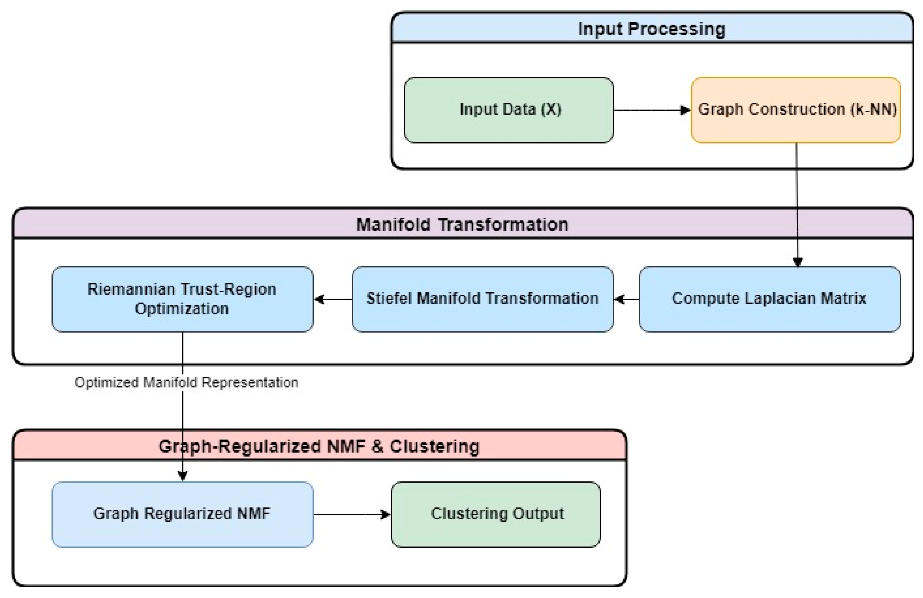
3. The SGRiT Algorithm

In this work, we present a novel algorithm that introduces constraints to enhance the standard NMF framework. This algorithm operates within the Stiefel manifold and an orthogonal subspace by leveraging the Riemannian trust region algorithm. Our approach combines a low-rank constraint on the transferred data, sparsity, and a graph smoothness constraint on the coefficient matrix. The workflow of the SGRiT approach is illustrated in Figure 1.

Let the data matrix be denoted as X = [x₁, x₂, …, x_N] ∈ R_N×M, where x_i,j ≥ 0. The widely used Spectral Clustering (SC) [20] technique involves the following steps to create a new representation of data:

• Construct a matrix W of pairwise similarities among N points based on algorithms like K-NN.
• The normalized graph Laplacian is as follows:

$$\mathrm{L}=\mathrm{I}-{\mathrm{D}}^{-1/2}\mathrm{W}{\mathrm{D}}^{-1/2}$$

where D is the diagonal matrix with the following:

$${\mathrm{d}}_{\mathrm{i}\mathrm{i}}={\sum }_{\mathrm{j}=1}^{\mathrm{N}}{\mathrm{W}}_{\mathrm{i}\mathrm{j}}$$

3.

The optimization problem for computing Y ∈ R^N×d, d << M is as follows:

$$\mathrm{m}\mathrm{i}\mathrm{n}<\mathrm{Y}{\mathrm{Y}}^{\mathrm{T}}, \mathrm{L}> \mathrm{s}.\mathrm{t} \mathrm{Y}\in {\mathrm{R}}^{\mathrm{N}\times \mathrm{d}}, {\mathrm{Y}}^{\mathrm{T}}\mathrm{Y}=\mathrm{I}$$

(1)

where Y is the d-dimensional new representation in new subspace of M-dimensional original data X in original subspace and $<\mathrm{Y}{\mathrm{Y}}^{\mathrm{T}},\mathrm{L}>$ denotes the inner product which generalizes the standard dot product to matrices. The definition of Stiefel manifold that consist of all the orthogonal column matrix is as follows:

$$\mathrm{S}\mathrm{t}\left(\mathrm{d},\mathrm{N}\right)=\left\{\mathrm{Y}\in {\mathrm{R}}^{\mathrm{N}\times \mathrm{d}}\right|\mathrm{Y}{\mathrm{Y}}^{\mathrm{T}}=\mathrm{I}\}.$$

(2)

By comparing relations (1) and (2), it is clear that problem (1) is an unconstrained manifold optimization problem on the Stiefel manifold S(d,N). Thus, the unconstrained manifold optimization problem (1) on the Stiefel manifold can be written as follows:

$$\mathrm{m}\mathrm{i}\mathrm{n}<\mathrm{Y}{\mathrm{Y}}^{\mathrm{T}},\mathrm{L}> \mathrm{s}.\mathrm{t} \mathrm{Y}\in {\mathrm{R}}^{\mathrm{N}\times \mathrm{d}},\mathrm{Y}\in \mathrm{S}\mathrm{t}\left(\mathrm{d},\mathrm{N}\right)$$

(3)

The Riemannian trust-region algorithm is employed on the Stiefel manifold optimization Equation (3), yielding a new representation data matrix Y. This involves using the pymanopt (https://pymanopt.org/) package in the python programming language to convert the original data space to a new orthogonal subspace through the largest k eigenvectors corresponding to the top k eigenvalues of W.

Subsequently, the nearest neighborhood graph is recreated from new representation data matrix Y with the improved-weighted matrix W. This new matrix W and new subspace representation of data is employed in the NMF process, incorporating the graph smoothness and sparsity constraint to partition data into clusters.

The NMF decomposes each observed data point X into two nonnegative matrices U ϵ ${\mathrm{R}}_{+}^{\mathrm{N}\ast \mathrm{d}}$ and V ϵ ${\mathrm{R}}_{+}^{\mathrm{d}\ast \mathrm{M}}$. U acts as the coefficient matrix, and V serves as the basis matrix in tasks like clustering. The core objective is to minimize the square of the Euclidean distance under non-negativity constraints:

$${\mathrm{O}}_{\mathrm{F}}={\mathrm{m}\mathrm{i}\mathrm{n}}_{\mathrm{U},\mathrm{V}}{\left|\left|\mathrm{X}-\mathrm{U}\mathrm{V}\right|\right|}_{\mathrm{F}}^2$$

$$\mathrm{s}.\mathrm{t}.\mathrm{U}\ge 0, \mathrm{V}\ge 0$$

Orthogonal Non-negative Matrix Factorization (ONMF) models can impose orthogonality on the basis matrices for parts-based interpretation.

$${\mathrm{m}\mathrm{i}\mathrm{n}}_{\mathrm{U},\mathrm{V}}\left|\right|\mathrm{X}-\mathrm{U}\mathrm{V}|{|}_{\mathrm{F}}^2$$

$$\mathrm{s}.\mathrm{t}.\mathrm{U}\ge 0, \mathrm{V}\ge 0, \mathrm{V}{\mathrm{V}}^{\mathrm{T}}=\mathrm{I}$$

When the SGRiT algorithm transfers original data into a subspace on Stiefel manifold with orthogonal vectors, it disregards the orthogonality of basis matrix V and writes the optimization equation accordingly.

$${\mathrm{m}\mathrm{i}\mathrm{n}}_{\mathrm{U},\mathrm{V}}\left|\right|\mathrm{n}\mathrm{e}\mathrm{w}\text{\_}\mathrm{X}-\mathrm{U}\mathrm{V}|{|}_{\mathrm{F}}^2$$

$$\mathrm{s}.\mathrm{t}.\mathrm{U}\ge 0, \mathrm{V}\ge 0$$

The algorithm enhances sparsity by introducing an independent penalty term, making the basis vectors sparser:

$${\mathrm{m}\mathrm{i}\mathrm{n}}_{\mathrm{U},\mathrm{V}}\left|\right|\mathrm{n}\mathrm{e}\mathrm{w}\text{\_}\mathrm{X}-\mathrm{U}\mathrm{V}|{|}_{\mathrm{F}}^2+|\left|\mathrm{U}\right|{|}_{\mathrm{F}}^2$$

$$\mathrm{s}.\mathrm{t}.\mathrm{U}\ge 0, \mathrm{V}\ge 0$$

To maintain the local geometric structure of the data manifold, it incorporates the graph smoothness regularization term into the objective function. However, instead of using the Laplacian matrix, which is made from the similarity matrix of the original data, it uses the Laplacian matrix, which is made from the transferred data under the Stiefel manifold and with the help of Riemannian optimization. This ensures that the geometric structure of the data is preserved better, leading to more accurate clustering results.

$${{\mathrm{O}}_{\mathrm{F}}=\mathrm{m}\mathrm{i}\mathrm{n}}_{\mathrm{U},\mathrm{V}}\left|\right|\mathrm{n}\mathrm{e}\mathrm{w}\text{\_}\mathrm{X}-\mathrm{U}\mathrm{V}|{|}_{\mathrm{F}}^2+\mathsf{\alpha }\mathrm{T}\mathrm{r}({\mathrm{U}}^{\mathrm{T}}{\mathrm{L}}_{\mathrm{n}\mathrm{e}\mathrm{w}\text{\_}\mathrm{x}}\mathrm{U})+\mathsf{\beta }|\left|\mathrm{U}\right|{|}_{\mathrm{F}}^2$$

(4)

$$\mathrm{s}.\mathrm{t}.\mathrm{U}\ge 0, \mathrm{V}\ge 0$$

Finally, the parameters α and β control the weight of the graph smoothness and sparsity regularization terms, respectively.

Optimization

To minimize the objective function presented in Equation (4), the algorithm calculates the derivatives of this function with respect to U while keeping V fixed and with respect to V while keeping U fixed in the Euclidean space.

$${\displaystyle \frac{\partial \left(\mathrm{O}\mathrm{F}\right)}{\partial \left(\mathrm{U}\right)}}=-2\mathrm{X}{\mathrm{V}}^{\mathrm{T}}+2\mathrm{U}\mathrm{V}{\mathrm{V}}^{\mathrm{T}}+2\mathsf{\alpha }\mathrm{D}\mathrm{U}-2\mathsf{\alpha }\mathrm{W}\mathrm{U}+2\mathsf{\beta }\mathrm{U}$$

$${\displaystyle \frac{\partial \left(\mathrm{O}\mathrm{F}\right)}{\partial \left(\mathrm{V}\right)}}=-2{\mathrm{U}}^{\mathrm{T}}\mathrm{X}+2{\mathrm{U}}^{\mathrm{T}}\mathrm{U}\mathrm{V}$$

where L is replaced with L = D − W.

Using the KKT condition and KKT complementary slackness, which is as follows:

$$\mathrm{U}\mathrm{ʘ}{\displaystyle \frac{\partial \left(\mathrm{O}\mathrm{F}\right)}{\partial \left(\mathrm{U}\right)}}=0$$

$$\mathrm{V}\mathrm{ʘ}{\displaystyle \frac{\partial \left(\mathrm{O}\mathrm{F}\right)}{\partial \left(\mathrm{V}\right)}}=0$$

The symbols ⊙ and the fraction line ($\frac{ }{ }$) indicate element-wise matrix product and division, respectively. According to the above equations, the multiplicative update rules for U and V are given by the following:

$${\mathrm{U}}_{\mathrm{t}+1}\leftarrow {\mathrm{U}}_{\mathrm{t}}\odot {\displaystyle \frac{\mathrm{X}{\mathrm{V}}_{\mathrm{t}}^{\mathrm{T}}+\mathsf{\alpha }\mathrm{W}{\mathrm{U}}_{\mathrm{t}}}{{\mathrm{U}}_{\mathrm{t}}{\mathrm{V}}_{\mathrm{t}}{\mathrm{V}}_{\mathrm{t}}^{\mathrm{T}}+\mathsf{\alpha }\mathrm{D}{\mathrm{U}}_{\mathrm{t}}+\mathsf{\beta }{\mathrm{U}}_{\mathrm{t}}}}$$

$${\mathrm{V}}_{\mathrm{t}+1}\leftarrow {\mathrm{V}}_{\mathrm{t}}\odot {\displaystyle \frac{{\mathrm{U}}_{\mathrm{t}}^{\mathrm{T}}\mathrm{X}}{{\mathrm{U}}_{\mathrm{t}}^{\mathrm{T}}{\mathrm{U}}_{\mathrm{t}}{\mathrm{V}}_{\mathrm{t}}}}$$

Therefore, the whole above process can be implemented in the form of Algorithm 1. The SGRiT method is expressed as an optimization problem that is resolved through an iterative multiplicative algorithm.

Algorithm 1: The SGRiT Algorithm
Input:  • Nonnegative data matrix X  • k for K-Nearest-Neighbors algorithm  • Parameters α and β Output:  • Nonnegative factor matrix U as the clustering result Steps:
	Compute the (weighted) graph W using the k-Nearest-Neighbors approach for normalized points in X. Calculate the diagonal matrix D based on the graph W and normalized graph Laplacian as follow: $$\mathrm{L}=\mathrm{I}-{\mathrm{D}}^{-1/2}\mathrm{W}{\mathrm{D}}^{-1/2}$$ 3. Utilize the pymanopt library to project the original data X onto a Stiefel manifold subspace Y with Euclidean distances based of relation (3) 4. Compute the (weighted) graph W and the diagonal matrix D based on the new data in the newly formed subspace. 5. repeat $${\mathrm{U}}_{\mathrm{t}+1}\leftarrow {\mathrm{U}}_{\mathrm{t}}\odot {\displaystyle \frac{\mathrm{Y}{\mathrm{V}}_{\mathrm{t}}^{\mathrm{T}}+\mathsf{\alpha }\mathrm{W}{\mathrm{U}}_{\mathrm{t}}}{{\mathrm{U}}_{\mathrm{t}}{\mathrm{V}}_{\mathrm{t}}{\mathrm{V}}_{\mathrm{t}}^{\mathrm{T}}+\mathsf{\alpha }\mathrm{D}{\mathrm{U}}_{\mathrm{t}}+\mathsf{\beta }{\mathrm{U}}_{\mathrm{t}}}}$$ $${\mathrm{V}}_{\mathrm{t}+1}\leftarrow {\mathrm{V}}_{\mathrm{t}}\odot {\displaystyle \frac{{\mathrm{U}}_{\mathrm{t}}^{\mathrm{T}}\mathrm{Y}}{{\mathrm{U}}_{\mathrm{t}}^{\mathrm{T}}{\mathrm{U}}_{\mathrm{t}}{\mathrm{V}}_{\mathrm{t}}}}$$ $\mathrm{t}\leftarrow \mathrm{t}+1$, until the convergence criterion is satisfied 6. apply kmeans to Ut+1 7. return Ut+1

4. Experiments and Analysis

In this section, a series of experiments have been conducted to validate and analyze the algorithm’s performance across various dimensions. These experiments include algorithm parameter selection analysis as well as clustering effect comparison. To ensure comprehensive validation, the outcomes of the SGRiT algorithm have been compared against those of other Non-negative Matrix Factorization (NMF) algorithms.

4.1. Datasets

Clustering experiments are executed on ten distinct datasets, for which the statistical information is presented in

Table 1. Dataset specification.

Dataset	# Instances	# Attribute	# Clusters	Subject Area	Attribute Type
Breast	683	9	2	Life	Integer (0–10)
Pendigit	477	16	3	Image	Integer (0–100)
Yale	165	1024	15	Image	Integer (0–255)
Optdigits	5620	64	10	Image	Integer (0–16)
Coil20	1440	1024	20	Image	Real (0–1)
ORL	400	10304	40	Image	Integer (0–255)
Ecoli	327	7	5	Gene exp.	Real (0–1)
Isolet	6238	617	26	Speech	Real (−1–1)
CNAE_9	1080	857	9	Business—text	Real (0–1)
USPS	9298	256	10	Image	Real (0–1)

.

4.2. Compared Algorithms

To ensure a fair and rigorous comparison of the SGRiT algorithm’s performance, it has been benchmarked against six other classic NMF algorithms. Below, a comprehensive description of each of these comparison algorithms is provided.

NMF: The classic Non-negative Matrix Factorization algorithm that enforces non-negativity constraints on the two factor matrices produced during decomposition.

SNMF: The Sparse Non-negative Matrix Factorization (SNMF) algorithm incorporates sparsity constraints into the standard NMF framework to improve parts-based learning. These constraints significantly enhance the discriminative power of the learned components. Additionally, SNMF introduces a more streamlined representation approach.

RNMF: Robust Non-negative Matrix Factorization (RNMF) is a variant of the NMF algorithm specifically designed to manage datasets that may contain outliers or noise. RNMF addresses these challenges by introducing sparsity constraints on the residual matrix. The concept of sparsity in RNMF is grounded in the understanding that noise or outliers are typically sparse and affect only a limited number of data points. By incorporating these sparsity constraints, RNMF effectively separates the clean data components from the corrupted ones, resulting in more accurate factorization outcomes.

PNMF: Probabilistic Non-negative Matrix Factorization (PNMF) employs variational Bayesian inference to achieve deterministic convergence to the solution of NMF, moving away from dependence on random sampling.

ONMF: Orthogonal Non-negative Matrix Factorization (ONMF) is based on the principles of standard NMF. Ref. [42] introduced ONMF models that incorporate orthogonality constraints on both the basis and coefficient matrices.

GNMF: Graph Regularized Non-negative Matrix Factorization (GNMF) constructs the local geometric structure of the original data space and incorporates it into the classic NMF algorithm as constraints, effectively utilizing it as a regularization term.

LNMFS: The Low-Rank NMF on the Stiefel Manifold (LNMFS) algorithm, as proposed by [7], utilizes the low-rank structure of intrinsic data and represents it in a Frobenius norm format using latent factors. Additionally, it maintains orthogonality among the factors by ensuring that the basis matrix lies on a Stiefel manifold. Furthermore, it incorporates a graph smoothness constraint on the coefficient matrix.

4.3. Parameter Analysis

In this analysis, specific parameters were evaluated to understand their influence on the algorithm’s performance. Reference [7] demonstrated that an increase in embedding dimension does not necessarily lead to improved clustering performance. Instead, optimal or nearly optimal clustering performance is typically achieved when the embedding dimension aligns with the number of clusters. This observation can be attributed to the fact that matching the embedding dimension with the rank of the intrinsic data allows for the maximal utilization of the low-rank regularization term. Therefore, for each dataset, the dimension of the matrix decomposition’s embedding was set as equal to the number of clusters, ensuring that each dimension of the latent feature space corresponds to a distinct cluster.

Three parameters in the algorithm under evaluation need to be adjusted. First, the square root of the number of samples per cluster is used to define the parameter ’k’, which is employed to calculate the graph of k-nearest neighbors within the k-NN algorithm. To create a binary adjacency matrix that captures the relationships between data items based on their shared nearest neighbors, 0/1 neighbor graphs are constructed. The adjacency matrix is denoted as W, where each element w_ij indicates the connection strength between the ith and jth data points.

Given that the SGRiT algorithm and LNMFS operate under the assumption that the basis vectors are orthogonal during the decomposition procedure, a specific initialization strategy is employed. Specifically, the V matrix is initialized by generating a random orthogonal matrix, while the U matrix is initialized using random values. This approach allows for flexibility in the initial configuration of U while still adhering to the requirements of the optimization process’s requirements. The orthogonal initialization of V and the randomized initialization of U collectively enhance the algorithm’s capacity to converge towards a solution that conforms to the orthogonal basis vector assumption and effectively approximates the original data matrix.

The optimal values for the coefficients ‘α’ and ‘β’, which, respectively, represent the weights of the geometric structure and sparsity terms in the objective function, were identified through experimentation on diverse datasets. Values ranging from 10⁻⁵ to 10⁺⁵ were examined in intervals of 10^0.5. The average purity attained for different ‘α’ and ‘β’ values across various datasets was computed, and the maximum of these averages was deemed the suitable ‘α’ and ‘β’ for the algorithm. For the LNMFS algorithm, the optimal values were found to be α = 1 and β = 10^2.5, while, for the SGRiT algorithm, the values were α = 0.1 and β = 10^3.5. α and β are parameters that influence the smoothness and sparsity of the data in relation to the value derived from the Frobenius norm. Our results indicate that, although these parameters exhibit some dependence on the data, they can be assigned values that produce acceptable outputs across all datasets. All datasets have been normalized by dividing by the maximum of each column so that different features have the same weight in the evaluation algorithms.

4.4. Evaluation Metrics

To evaluate the performance of the SGRiT algorithm in comparison to the other selected algorithms, four key assessment criteria are utilized: Purity, Normalized Mutual Information (NMI), Rand Index, and algorithm execution time.

Purity: Purity is a straightforward and transparent evaluation metric, especially in the context of unsupervised machine learning. It involves assigning each cluster to the class that is most prevalent within that cluster. The accuracy of this assignment is calculated by dividing the number of correctly assigned objects by the total number of objects in the dataset. High purity values indicate effective clustering, with perfect clustering achieving a purity of 1, while poor clustering results in purity values close to 0. However, it is important to note that high purity can be easily achieved when the number of clusters is large; therefore, purity alone may not be the best metric for balancing clustering quality against the number of clusters.

The purity of a clustering result is calculated using the following equation:

$$\mathrm{p}\mathrm{u}\mathrm{r}\mathrm{i}\mathrm{t}\mathrm{y}={\displaystyle \frac{1}{\mathrm{N}}}\sum _{\mathrm{i}=1}^{\mathrm{k}}{\mathrm{m}\mathrm{a}\mathrm{x}}_{\mathrm{j}}|{\mathrm{C}}_{\mathrm{i}}\cap {\mathrm{L}}_{\mathrm{j}}|$$

where:

N is the total number of data points.

K is the number of clusters in the clustering result.

C_i is the set of data points in cluster i.

L_j is the set of data points in class j according to the ground-truth labels.

The purity is calculated by summing over each cluster i and finding the maximum overlap between that cluster and any class j based on ground-truth labels. The result is normalized by dividing by the total number of data points N.

Normalized Mutual Information (NMI): NMI allows us to strike a balance between clustering quality and the number of clusters, as it is independent of the cluster count. It can be information-theoretically interpreted and quantifies the average mutual information between each pair of clusters and classes, while also considering the normalization factors to make it a value between 0 and 1.

The formula for NMI is as follows:

$$\mathrm{N}\mathrm{M}\mathrm{I}={\displaystyle \frac{\mathrm{I}(\mathrm{C};\mathrm{L})}{\sqrt{\mathrm{H}\left(\mathrm{C}\right).\mathrm{H}\left(\mathrm{L}\right)}}}$$

where

I(C; L) is the mutual information between the clustering C and the reference labels L.

H(C) is the entropy of the clustering C.

H(L) is the entropy of the reference labels L.

Rand Index (RI): Rand Index (RI) is a metric used to measure the similarity between two data clustering. It takes into account both false positive (FP) and false negative (FN) decisions during clustering evaluation. It measures the percentage of decisions that are correct (true positives + true negatives) out of the total decisions. It provides a value between 0 and 1, where higher values indicate greater similarity between the clustering.

$$\mathrm{R}\mathrm{I}={\displaystyle \frac{\mathrm{T}\mathrm{P}+\mathrm{T}\mathrm{N}}{\mathrm{T}\mathrm{P}+\mathrm{F}\mathrm{P}+\mathrm{F}\mathrm{N}+\mathrm{T}\mathrm{N}}}$$

These evaluation criteria collectively provide a comprehensive understanding of the performance of the SGRiT algorithm compared to other algorithms. In such cases, optimizing for accuracy alone may not provide a clear picture of model performance, as a classifier can achieve high accuracy by simply predicting the majority class for all instances.

4.5. Clustering Results Analysis

To evaluate the clustering results of NMF, SNMF, RNMF, PNMF, ONMF, GNMF, LNMFS, and the SGRiT algorithm, the five previously mentioned evaluation criteria have been employed. The implementations of NMF, SNMF, RNMF, PNMF, and ONMF are sourced from NMF library packages https://github.com/hiroyuki-kasai/NMFLibrary (accessed on 10 March 2025), while the code for LNMFS and the SGRiT algorithm is developed within the Python environment. To ensure reliable results, each algorithm is executed ten times, and the average value of the criteria, along with their standard deviation, is computed. Instances where an algorithm fails to produce clustering results are indicated by NA.

The results presented in

Table 2. Comparison of NMF clustering algorithms using purity criterion.

Dataset	NMF	SNMF	RNMF	PNMF	ONMF	GNMF	LNMFS	SGRiT
Breast	0.9487 ±0.0163	0.9652 ±0.0017	0.9387 ±0.0296	0.9223 ±0.0606	0.9580 ±0.0053	0.9622 ±0.00092	0.966325 ±0.00	0.972329 ±0.00138
Pendigit	0.7544 ±0.0922	0.6878 ±0.0861	0.6990 ±0.0967	0.7071 ±0.0580	0.6853 ±0.0859	0.6688 ±0.1082	0.825996 ±0.00	0.931343 ±0.00091
Yale	0.4206 ±0.0373	0.3764 ±0.0163	0.4285 ±0.0259	0.3206 ±0.0288	0.4564 ±0.0406	0.3970 ±0.0261	0.47151 ±0.019601	0.491516 ±0.02072
Optdigit	0.7192 ±0.0376	0.7010 ±0.0260	0.7164 ±0.0268	0.5041 ±0.0597	0.7082 ±0.0290	0.8177 ±0.0317	0.81173 ±0.003058	0.851761 ±0.04277
coil20	0.6506 ±0.0354	0.6551 ±0.0338	0.6542 ±0.0294	0.4433 ±0.0212	0.6445 ±0.0307	0.6478 ±0.0365	0.728125 ±0.018930	0.767049 ±0.021013
ORL	0.6603 ±0.0337	0.3912 ±0.0185	0.4172 ±0.0085	0.2393 ±0.0150	0.6647 ±0.0321	0.7215 ±0.0349	0.77012 ±0.01558	0.79825 ±0.01210
Ecoli	0.7803 ±0.0270	0.7653 ±0.0305	0.7659 ±0.0316	0.5304 ±0.0334	0.7888 ±0.0128	0.7920 ±0.0129	0.76514 ±0.00183	0.78547 ±0.04113
Isolet	0.5817 ±0.0246	0.2673 ±0.0059	0.5695 ±0.0167	0.1203 ±0.0064	0.5069 ±0.0203	0.4858 ±0.0177	0.58994 ±0.01048	0.59396 ±0.00916
USPS	0.6867 ±0.0247	0.5994 ±0.0266	0.6661 ±0.0228	0.5433 ±0.0266	0.6389 ±0.0237	0.6953 ±0.0511	0.72768 ±0.00029	0.76886 ±0.03543
CNAE	0.4951 ±0.0310	0.3282 ±0.0440	NA	NA	0.4575 ±0.0365	0.5336 ±0.0390	0.92324 ±0.03028	0.97778 ±0.03493

clearly demonstrate that the SGRiT algorithm exhibits the highest purity across most datasets when compared to various other algorithms. With the exception of the Ecoli dataset, which is ranked third, the SGRiT method consistently secures the top position in all other instances. Ecoli is a relatively simple dataset characterized by low dimensionality, a limited number of samples, and five classes. This simplicity makes the dataset more amenable to less complex approaches, while the SGRiT method excels on more complex datasets that feature higher dimensionality and a greater number of classes. For instance, as illustrated in the results, the SGRiT approach significantly outperforms other methods on high-dimensional datasets such as Yale, Coil24, and ORL. A similar trend is observed in larger datasets with more instances and classes, including Isolet, CNAE, and USPS. Notably, in the case of the Pendigit dataset, the performance difference between SGRiT and the next-best algorithm reaches approximately 0.11. This indicates that the SGRiT algorithm achieves superior clustering performance in terms of the purity metric across a variety of datasets.

The standard deviations (SDs) of the experiments for the SGRiT approach are relatively low, indicating a high probability of convergence. In contrast to the mean performance, which was significantly better on more complex datasets, the SD is lower (i.e., nearly zero) for simpler datasets such as Breat and Pendigit. This observation suggests that the approach is both robust and stable; however, its stability diminishes as the complexity of the data increases. The NMI criterion quantifies the amount of information shared between two clustering results while accounting for random chance agreement. A higher NMI value indicates that the clusters produced by the algorithm correspond more closely with the true underlying structure or ground truth. The results of the tests concerning the NMI criterion, as presented in

Table 3. Comparison of NMF clustering algorithms using NMI criterion.

Dataset	NMF	SNMF	RNMF	PNMF	ONMF	GNMF	LNMFS	SGRiT
Breast	0.7010 ±0.0578	0.7695 ±0.0084	0.6693 ±0.1014	0.6335 ±0.1773	0.7374 ±0.0241	0.7563 ±0.0043	0.77644 ±0	0.809281 ±0.00783
Pendigit	0.5100 ±0.0763	0.4877 ±0.0647	0.4832 ±0.0600	0.4194 ±0.0442	0.4778 ±0.0680	0.4984 ±0.0870	0.57205 ±0	0.764918 ±0.00386
yale	0.4706 ±0.0372	0.4584 ±0.0192	0.4726 ±0.0199	0.3693 ±0.0243	0.5349 ±0.0343	0.4521 ±0.0164	0.522265 ±0.01462	0.535772 ±0.01564
optdigit	0.6410 ±0.0247	0.6298 ±0.0204	0.6484 ±0.0181	0.4312 ±0.0403	0.6442 ±0.0197	0.8450 ±0.0138	0.780463 ±0.00173	0.861650 ±0.02463
coil20	0.7407 ±0.0220	0.7268 ±0.0219	0.7447 ±0.0112	0.5280 ±0.0144	0.7547 ±0.0103	0.7895 ±0.0157	0.800294 ±0.01080	0.837761 ±0.01058
ORL	0.8185 ±0.0146	0.6070 ±0.0132	0.6288 ±0.0053	0.4783 ±0.0133	0.8241 ±0.0153	0.8514 ±0.0173	0.87994 ±0.00715	0.90363 ±0.00552
Ecoli	0.5636 ±0.0377	0.5811 ±0.0347	0.5534 ±0.0544	0.1442 ±0.0464	0.6103 ±0.0176	0.6026 ±0.0233	0.53857 ±0.00045	0.62357 ±0.0544
Isolet	0.6941 ±0.0179	0.3866 ±0.0056	0.6874 ±0.0105	0.1743 ±0.0160	0.6356 ±0.0143	0.6403 ±0.0132	0.72796 ±0.00567	0.73085 ±0.00832
USPS	0.5908 ±0.0151	0.4919 ±0.0176	0.5805 ±0.0125	0.4593 ±0.0251	0.5259 ±0.0261	0.7039 ±0.0258	0.64093 ±0.00021	0.74877 ±0.02032
CNAE	0.4466 ±0.0226	0.2508 ±0.0368	-	-	0.4146 ±0.0332	0.5498 ±0.0287	0.88802 ±0.01470	0.97892 ±0.01862

, demonstrate the superiority of the SGRiT algorithm across all selected datasets.

The observations presented in Table 2 are reiterated here, with the notable exception that the approach has excelled across all datasets. Table 2 indicates that SGRiT consistently outperforms other algorithms, achieving the highest NMI scores across all datasets, such as 0.809281 for the Breast dataset and 0.97892 for CNAE. In contrast, PNMF generally exhibits the poorest performance, with significantly low scores. Most algorithms, including GNMF and LNMFS, demonstrate competitive results, with GNMF particularly excelling on datasets such as Optdigit (0.8450) and ORL (0.8514). Overall, SGRiT showcases superior clustering accuracy and stability, as evidenced by its high NMI scores and relatively low standard deviations.

As observed, the margin of performance improvement based on the NMI criterion is notably higher in this context. For instance, on the Pendigit dataset, the improvement margin is 0.19; on the Ecoli and CANE datasets, the NMI improves by 0.09; on the USPS dataset, a 0.1 improvement is recorded. Referring to Table 1, both CANE and USPS are classified as complex datasets, and this performance enhancement further underscores the effectiveness of the SGRiT approach. The Rand Index (RI), a metric used to evaluate the similarity between two clustering or partitioning results, quantifies the agreement between the clustering assignments of elements within a dataset. It takes into account both pairs of elements that are correctly grouped together and pairs that are accurately placed in separate clusters.

As shown in

Table 4. Comparison of NMF clustering algorithms using Rand Index criterion.

Dataset	NMF	SNMF	RNMF	PNMF	ONMF	GNMF	LNMFS	SGRiT
breastw	0.9030 ±0.0279	0.9326 ±0.0031	0.8862 ±0.0503	0.8630 ±0.0953	0.9194 ±0.0098	0.9272 ±0.0017	0.93482 ±0.0	0.946114 ±0.00261
pendigit	0.7433 ±0.0673	0.7012 ±0.0607	0.7043 ±0.0679	0.7289 ±0.0289	0.7049 ±0.0683	0.6991 ±0.0796	0.80197 ±0.0	0.91478 ±0.00119
yale	0.8970 ±0.0105	0.8837 ±0.0079	0.9003 ±0.0035	0.8799 ±0.0085	0.9006 ±0.0117	0.8953 ±0.0032	0.902683 ±0.00542	0.902687 ±0.00583
optdigit	0.9154 ±0.0089	0.9137 ±0.0083	0.9162 ±0.0063	0.8692 ±0.0095	0.9144 ±0.0074	0.9498 ±0.0080	0.9455 ±0.00044	0.955102 ±0.01102
coil20	0.9526 ±0.0049	0.9503 ±0.0044	0.9524 ±0.0021	0.9201 ±0.0097	0.9520 ±0.0024	0.9499 ±0.0076	0.963807 ±0.00302	0.960247 ±0.00521
ORL	0.9752 ±0.0032	0.9599 ±0.0016	0.9609 ±0.007	0.9522 ±0.0016	0.9768 ±0.0024	0.9784 ±0.0041	0.98293 ±0.00122	0.98473 ±0.00146
Ecoli	0.8140 ±0.0322	0.8131 ±0.0289	0.8070 ±0.0318	0.6661 ±0.0158	0.8168 ±0.0251	0.8309 ±0.0340	0.7937 ±0.00056	0.84265 ±0.04616
Isolet	0.9576 ±0.0026	0.9324 ±0.0010	0.9565 ±0.0021	0.9286 ±0.0003	0.9511 ±0.0021	0.9454 ±0.0041	0.95985 ±0.00150	0.94361 ±0.00233
USPS	0.9026 ±0.0064	0.8836 ±0.0064	0.9001 ±0.0046	0.8754 ±0.0069	0.8892 ±0.0075	0.8960 ±0.0177	0.91500 ±0.00001	0.92104 ±0.00985
CNAE	0.7684 ±0.0479	0.7550 ±0.0366	-	-	0.7653 ±0.0330	0.7911 ±0.0153	0.96996 ±0.00766	0.99123 ±0.01106

, with the exception of the Isolet dataset, where the SGRiT algorithm ranks lower (sixth place), the algorithm consistently achieves either first or second place in the remaining cases. Notably, SGRiT attains the highest Rand Index scores, such as 0.99123 for CNAE and 0.98473 for ORL, indicating superior clustering accuracy. In contrast, PNMF generally performs the worst, with particularly low scores of 0.6661 for Ecoli and 0.8630 for breast cancer. Most algorithms, including GNMF and LNMFS, yield competitive results, with GNMF performing exceptionally well on datasets like Optdigit (0.9498) and ORL (0.9784). Overall, SGRiT demonstrates the best performance, with high Rand Index values and relatively low standard deviations, underscoring its robustness and effectiveness. This performance may be attributed to the presence of negative data in the dataset. To align with the principles of the NMF algorithm, the SGRiT algorithm adds the minimum value of the data to all entries, ensuring that the resulting matrix is positive and suitable for NMF implementation. This observation suggests that, for the majority of datasets, the proposed clustering algorithm exhibits satisfactory performance in terms of the Rand Index criterion. Additionally, the standard deviation of the resulting Rand Index reflects the stability and robustness of the approach across different learning subsets.

Time complexity analysis in NMF is crucial, as the algorithms can be computationally intensive, particularly when handling large datasets. Analyzing time complexity aids in selecting or designing algorithms that can efficiently factorize matrices, thereby conserving computational resources. Furthermore, understanding time complexity enables researchers and practitioners to evaluate the scalability of NMF algorithms, which is essential when working with large datasets or high-dimensional matrices. Therefore, a run-time analysis is performed and reported in this section. Experiments involving SGRiT and LNMFS algorithms were conducted using PyCharm version 2021.3.1 with Python version 3.11. For the other methods, MATLAB R2015a was employed. The experiments were carried out on a server equipped with an Intel Xeon E7530 processor operating at 1.87 GHz (56 processors) and 16 GB of RAM. To accurately measure the algorithm’s runtime, it was executed 10 times, and the average execution time for each algorithm was recorded in the table. As seen in

Table 5. Comparison of NMF clustering algorithms based on average runtime (seconds).

Dataset	NMF	SNMF	RNMF	PNMF	ONMF	GNMF	LNMFS	SGRiT
Breast	0.0616	0.3155	0.0650	1.1529	0.0766	0.0519	0.286093	3.267077
Pendigit	0.3019	0.3842	0.4104	0.6889	0.3282	0.0859	0.286484	3.471461
Yale	1.3183	1.4770	2.2548	1.0631	1.2387	28.9914	0.466393	11.74773
Optdigit	2.2166	6.4239	4.3264	74.2212	2.3242	4.5397	2.878699	175.2087
coil20	5.8945	10.3548	12.4063	11.2105	6.1838	93.4495	6.102626	1013.291
ORL	16.7005	27.5007	32.1867	19.1119	20.3024	76.4009	2.476567	164.5794
Ecoli	0.2872	0.4023	0.3409	0.3219	0.1921	0.1417	0.323091	3.596105
Isolet	17.4518	68.4546	32.3020	154.4711	17.5103	29.9876	6.889409	564.1962
USPS	9.3402	50.6754	19.7059	234.0410	9.2002	10.8237	6.508134	281.3154
CNAE	3.9827	6.4396	-	-	4.1527	4.2311	0.636361	9.70614

, the proposed algorithm takes a lot of time to transfer the data from the main space to a subspace with smaller dimensions; this problem causes a significant increase in the execution time of this algorithm compared to other algorithms, as in the practical test of all the data.

The experimental results clearly demonstrate that SGRiT consistently outperforms seven representative NMF-based algorithms; however, it is less efficient in terms of execution time for clustering tasks across a diverse range of real-world datasets. While SGRiT may exhibit longer execution times in certain scenarios, the additional computational cost is warranted by our primary objective of enhancing clustering performance. For applications where accuracy is prioritized over speed, the SGRiT algorithm focuses on achieving superior feature extraction and clustering quality. Moreover, NMF can be executed offline, mitigating the impact of prolonged execution times. Additionally, optimizations such as parallelization and approximation can be implemented to reduce computational costs when runtime efficiency is critical.

5. Conclusions

In this article, a new method for clustering using Non-negative Matrix Factorization is presented. This method transforms the primary data into a lower-dimensional subspace, which maintains orthogonality and is referred to as the Stiefel manifold space, utilizing a data transformation algorithm. To achieve this, the Riemannian trust region optimization algorithm is employed. The reduced-dimensional data provide clustering algorithms with enhanced insights into the hidden geometric structure of the data and its manifold. Experiments conducted on ten different datasets demonstrate that the proposed SGRiT algorithm outperforms traditional NMF-based algorithms in clustering performance in most cases. Furthermore, the application of this algorithm in the field of co-clustering can facilitate a more effective extraction of the structure and manifold of features, warranting further exploration in future research. Additionally, to enhance reliability, strategies to mitigate noise and outliers should also be addressed.