Electrical Storm Optimization (ESO) Algorithm: Theoretical Foundations, Analysis, and Application to Engineering Problems

Abstract

The electrical storm optimization (ESO) algorithm, inspired by the dynamic nature of electrical storms, is a novel population-based metaheuristic that employs three dynamically adjusted parameters: field resistance, field intensity, and field conductivity. Field resistance assesses the spread of solutions within the search space, reflecting strategy diversity. The field intensity balances the exploration of new territories and the exploitation of promising areas. The field conductivity adjusts the adaptability of the search process, enhancing the algorithm’s ability to escape local optima and converge on global solutions. These adjustments enable the ESO to adapt in real-time to various optimization scenarios, steering the search toward potential optima. ESO’s performance was rigorously tested against 60 benchmark problems from the IEEE CEC SOBC 2022 suite and 20 well-known metaheuristics. The results demonstrate the superior performance of ESOs, particularly in tasks requiring a nuanced balance between exploration and exploitation. Its efficacy is further validated through successful applications in four engineering domains, highlighting its precision, stability, flexibility, and efficiency. Additionally, the algorithm’s computational costs were evaluated in terms of the number of function evaluations and computational overhead, reinforcing its status as a standout choice in the metaheuristic field.

1. Introduction

Optimization constitutes a fundamental aspect of scientific research and engineering, aiming at identifying the most effective solution among a plethora of feasible options under given constraints [1,2,3,4]. It plays a pivotal role in decision-making processes across various domains, including logistics, manufacturing, finance, and artificial intelligence [5]. Most of the problems presented in different scientific and engineering areas can be formulated as optimization problems [6].

Various optimization problems are classified on the basis of their objective function nature, constraints, and variables involved [7,8,9]. Within the classification of optimization techniques, exact methods, which are designed to find the optimal solution with precision guarantees for certain problem types, represent a critical category [2]. Exact methods are particularly powerful in contexts where the requirements for accuracy and certainty outweigh the need for computational efficiency. However, these methods are not generally effective in solving complex optimization problems because of their dependency on preconditions such as continuity, convexity, and differentiability of the objective function, which are not usually met in real-world optimization problems [7,8,10,11]

The quest for a balance between computational efficiency and optimal solution finding has spurred significant interest in heuristic and metaheuristic methods [7,8,12]. These algorithms have proven effective at navigating complex search spaces to efficiently deliver near-optimal solutions [9,13,14,15]. In recent years, significant advancements in metaheuristic algorithms have been reported. Notable developments include the marine predator algorithm (MPA) [16], which models hunting strategies in marine ecosystems, and the equilibrium optimizer (EO) [17], which is based on mass balance principles. Henry gas solubility optimization (HGSO) [18] draws inspiration from gas solubility dynamics, whereas the modified artificial gorilla trout optimizer (MAGTO) [19] enhances primate behavior modeling. Tuna swarm optimization (TSO) [20] mimics tuna hunting patterns, and the rain optimization algorithm (ROA) [21] simulates precipitation processes. The modified Harris hawk optimization (MHHO) [22] improves upon cooperative hunting strategies. The Brown-Bear Optimization Algorithm (BBOA) [23] simulates the hunting and foraging behavior of brown bears, whereas the Energy Valley Optimizer (EVO) [24] draws inspiration from energy landscapes in physical systems. Fick’s law algorithm (FLA) [25] leverages principles of molecular diffusion, and the Honey Badger Algorithm (HBA) [26] models the aggressive foraging strategies of honey badgers. The Hunger games search (HGS) [27] implements competitive survival dynamics. Other significant contributions include the arithmetic optimization algorithm (AOA) [28], the modified whale optimization algorithm (MWOA) [29], and the enhanced leader particle swarm optimization (ELPSO). This proliferation of algorithms highlights both the field’s dynamism and the ongoing challenge of developing truly novel optimization mechanisms.

Despite the success of metaheuristics in addressing a broad spectrum of optimization challenges, the demand for more efficient, robust, and versatile algorithms persists, driven by increasingly complex optimization problems. As the field evolved through the late 20th and early 21st centuries, the number of metaheuristic algorithms grew to over 500 by the end of 2023, each designed to address specific complex issues [30]. Research suggests that many of the newly developed algorithms are enhancements or variations of existing methods [7,31,32] This trend highlights the iterative process of science but has also drawn several criticisms. A significant concern is the lack of novelty, with many new algorithms being minor modifications rather than genuine innovations [33]. Additionally, the introduction of biases, such as center bias, skews the performance results, favoring solutions near the center of the search space [34]. Another issue is the inconsistency between the proposed metaphors, mathematical models, and algorithm implementations. Often, the metaphors do not translate into the algorithm’s framework, leading to a disconnect between theory and practice [35]. Furthermore, the lack of consistent and transparent benchmarking complicates the assessment of algorithm efficacy [36]. Selective datasets and metrics can result in biased conclusions that fail in broader applications.

In this context, we introduce the electrical storm optimization (ESO) algorithm, a novel mathematical approach inspired by the dynamic behavior of electrical storms. This algorithm draws from the observation that lightning strikes the path of least resistance to ground, analogous to finding the optimal path through a complex search space. The ESO algorithm uses three dynamically adjusted parameters, field resistance, conductivity and intensity, to adapt the search process in real time. This allows the algorithm to seamlessly transition between the exploration and exploitation phases on the basis of the immediate needs of the optimization landscape. Unlike the reliance on interagent communication or fixed update mechanisms seen in other algorithms, the ESO approach is autonomously driven by environmental responses, increasing its adaptability across both discrete and continuous problem spaces. This study delineates the conceptual foundation of the ESO, its algorithmic structure, and potential implications for advancing the field of optimization.

The main objective of this study is to develop a robust and efficient optimization algorithm that can effectively handle both unimodal and multimodal optimization problems while maintaining consistent performance across varying dimensionalities. This work offers several key scientific contributions: (1) the introduction of a novel dynamic adaptation mechanism that automatically adjusts search parameters on the basis of real-time feedback from the optimization landscape, enabling seamless transitions between exploration and exploitation phases; (2) a self-regulating framework that reduces the need for parameter tuning across different problem types, enhancing the algorithm’s practical applicability; (3) a mathematically rigorous approach to distance-based resistance calculation that provides more accurate guidance for the search process; and (4) a computationally efficient implementation that scales well with problem dimensionality while maintaining competitive performance. These contributions address current limitations in the field of optimization algorithms, particularly in terms of adaptation capabilities and computational efficiency.

2. Materials and Methods

Thunderstorms are among the most potent phenomena in nature and are characterized by lightning occurring within cumulonimbus clouds. These clouds experience strong updrafts and downdrafts that move water particles across different altitudes. Collisions between droplets and ice particles, combined with temperature and pressure differences, lead to charge separation, the accumulation of positive charges at cloud tops and negative charges at the bases. This results in a strong electric field within the clouds and between the clouds and the surface of the Earth [37,38]. When the potential difference exceeds the dielectric strength of air, electrical discharge, known as lightning, occurs. This discharge, influenced by wind, humidity, and particulates, can occur within a cloud, between clouds, or from clouds to the ground and is subject to environmental obstacles such as terrain or structures, which can alter the path of lightning [39].

The ESO algorithm draws inspiration from these dynamics, particularly the way in which lightning seeks the path of least resistance. This natural process is applied to solve optimization problems, where the algorithm seeks optimal solutions by navigating through problem spaces in a manner analogous to lightning navigating atmospheric obstacles.

Field resistance ($R$): In thunderstorms, electrical resistance determines the ease with which lightning can travel through the different regions of the atmosphere [40,41]. In the ESO algorithm, this parameter measures the dispersion of solutions within the search space, guiding the algorithm’s adjustments on the basis of the problem’s topology.

Field intensity ($I$): The intensity of the electric field in a thunderstorm governs the strength and frequency of lightning discharges [42]. Analogously, this parameter controls the algorithmic phases, facilitating strategic shifts between exploration and exploitation.

Field conductivity ($ke$): Drawing from the concept of electrical conductivity, which measures the ability of a material or system to conduct electric current, this is the reciprocal of the resistance. Reflecting the adaptability required by lightning to navigate varying atmospheric conditions, this parameter dynamically modulates the algorithm’s response to changes in field resistance, enhancing its ability to fine-tune the search process.

Storm power ($P$): Storm power is inspired by the cumulative and finite potential energy present in a thunderstorm. In the ESO algorithm, P measures the remaining energy and potential for exploration during the search process. This ensures that the algorithm’s efforts are proportional to the current state of variability and intensity in the search space, maintaining an adaptive balance between exploration and exploitation.

Ionized areas ($\alpha$): In thunderstorms, ionized areas are regions where the air has become electrically conductive due to ionization, allowing for lightning to travel through these paths of least resistance [40,42]. In the ESO algorithm, the ionized areas represent regions in the search space where the probability of finding optimal solutions is higher. By identifying and targeting these ionized areas, the algorithm can navigate the search space more effectively, enhancing its efficiency in locating optimal solutions.

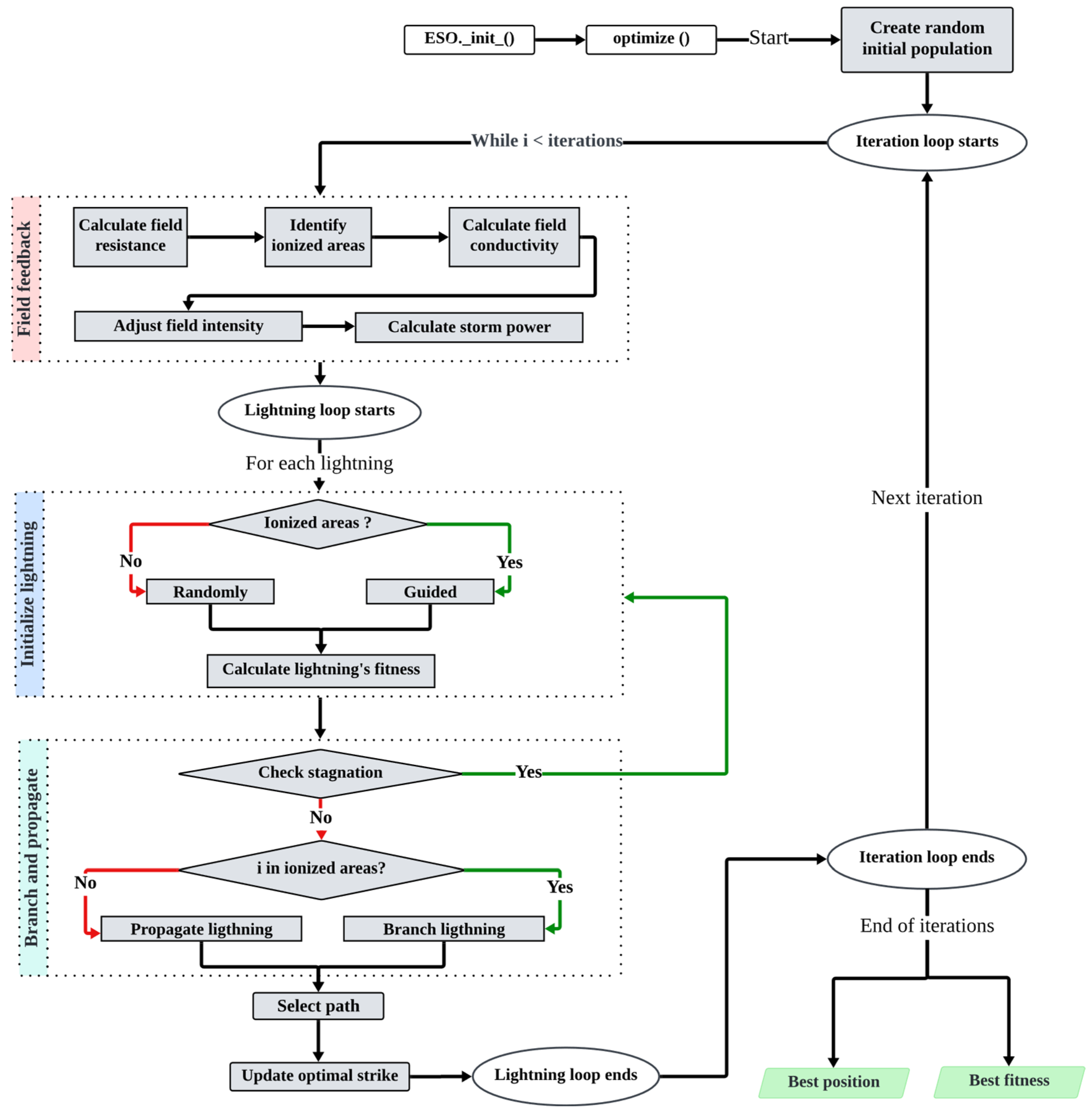
By leveraging nature-inspired dynamics, the ESO offers a structured and adaptive approach to complex optimization challenges, effectively translating these natural phenomena into computational strategies. Figure 1 illustrates how these dynamics are operationalized within the algorithm.

During the first iteration ($j=1$) of the optimization process, the lightning (agents) are positioned randomly within the defined lower ($b_{low}$) and upper ($b_{high}$) bounds of the search space with $n$ dimensions. This is expressed as ${\rho }_{i,j}^n$, where each agent $i$ is represented as a vector with both an origin and a direction that can explore the search space. Once these initial positions are established, the fitness of each lightning agent’s position is calculated by evaluating the objective function at the agent’s position. This initial assessment is crucial, as it sets the baseline for the algorithm’s iterative process of refining positions to find optimal solutions.

2.1. Field Resistance

The concept of field resistance ($R$) in the ESO algorithm is crucial for effectively managing the optimization process. It serves as a real-time feedback mechanism that reflects the landscape of the optimization problem, enabling the algorithm to dynamically control its operational phases. The field resistance is calculated as the ratio between the standard deviation ($\sigma$) and the peak-to-peak difference ($\mathsf{\Delta }p$) across these positions (${\rho }_{i,j}^n$) in each iteration ($j$) through the total lightning number ($N$), which is an argument of the algorithm. The standard deviation is computed on the basis of the deviation in each position from the mean position ($\overline{p}$), where $\overline{p}$ is the average of all the positions. The mathematical representation of this calculation is provided in Equations (1)–(3). A higher $R$ indicates a greater need for exploration, suggesting that the current solutions are widely spread and possibly distant from any optimum. Conversely, a lower $R$ indicates a denser clustering of solutions, suggesting its proximity to potential optima and thus a greater need for exploitation to fine-tune the solutions.

$${\mathit{\sigma }}_{\mathit{j}}=\sqrt{{\displaystyle \frac{1}{\mathit{N}-1}}{\sum }_{\mathit{i}=1}^{\mathit{N}}{\left({\mathit{\rho }}_{\mathit{i},\mathit{j}}^{\mathit{n}}-\overline{\mathit{p}}\right)}^2}$$

(1)

$${\mathit{\Delta }\mathit{p}}_{\mathit{j}}=\mathit{max}\left({\mathit{\rho }}_{\mathit{i}}^{\mathit{n}}\right)-\mathit{min}\left({\mathit{\rho }}_{\mathit{i}}^{\mathit{n}}\right)$$

(2)

$${\mathit{R}}_{\mathit{j}}={\displaystyle \frac{{\mathit{\sigma }}_{\mathit{j}}}{\mathit{max}\left({\mathit{\Delta }\mathit{p}}_{\mathit{j}}\right)}}$$

(3)

2.2. Ionized Areas

The ionized areas ($\mathsf{\alpha }$) are identified as the zones within the search space where the solutions are superior, indicating lower resistance. This involves selecting a subset of the best solutions on the basis of their fitness. First, the percentile of fitness from all the solutions is calculated via Equation (4). Then, the solutions whose fitness values are better (lower for minimization, higher for maximization) are selected, as expressed in Equation (5). This process ensures that the algorithm can identify and focus on the most promising areas of the search space, facilitating a more directed and potentially more efficient search.

$$\mathrm{percentile}=\left({\mathit{R}}_{\mathit{j}} | 2\right) \times \mathbf{100}$$

(4)

$$\mathsf{\alpha }=\mathit{solution} | {\mathit{f}\mathit{i}\mathit{t}\mathit{n}\mathit{e}\mathit{s}\mathit{s}}_{\mathit{s}}<\mathrm{percentile}\left(\mathrm{fitness}\right)$$

(5)

2.3. Field Conductivity

The field conductivity ($ke$) dynamically adjusts the search strategy in response to changes in $R$ in each iteration ($j$), allowing for the ESO algorithm to modulate exploration and exploitation on the basis of current environmental resistance. This parameter indicates how easily lightning can progress toward the optimum. It is computed via a logistic function ($\beta$), as expressed in Equations (6) and (7). The nonlinear nature of the logistic function makes $ke$ highly reactive to any small changes in $R$, allowing for quick and effective adjustments to the search strategy. This reactivity is essential for handling the variability and complexity of search spaces. A less responsive adjustment results in a slower convergence. High field resistance ($R)$ results in low $ke$, promoting exploration. Conversely, a low $R$ increases $ke$, favoring exploitation.

$${\mathit{\beta }}_{\mathit{j}} = {\displaystyle \frac{\mathbf{1}}{\mathbf{1}+{\mathit{e}}^{\left(-\left(\frac{{\mathit{e}}^{{\mathit{R}}_{\mathit{j}}}}{{\mathit{R}}_{\mathit{j}}}\right)\times \left({\mathit{R}}_{\mathit{j}}-\left|{\mathit{log}}_{\mathit{e}}\left(\mathbf{1}-{\mathit{R}}_{\mathit{j}}\right)\right|\right)\right)}}}$$

(6)

$${\mathit{k}\mathit{e}}_{\mathit{j}}={\mathit{e}}^{\left({\mathit{R}}_{\mathit{j}}\right)}+\left({\mathit{e}}^{\left(\mathbf{1}-{\mathit{R}}_{\mathit{j}}\right)}\times \left|{\mathit{log}}_{\mathit{e}}\left({\mathit{R}}_{\mathit{j}}\right)\right|\times {\mathit{\beta }}_{\mathit{j}}\right)$$

(7)

2.4. Field Intensity

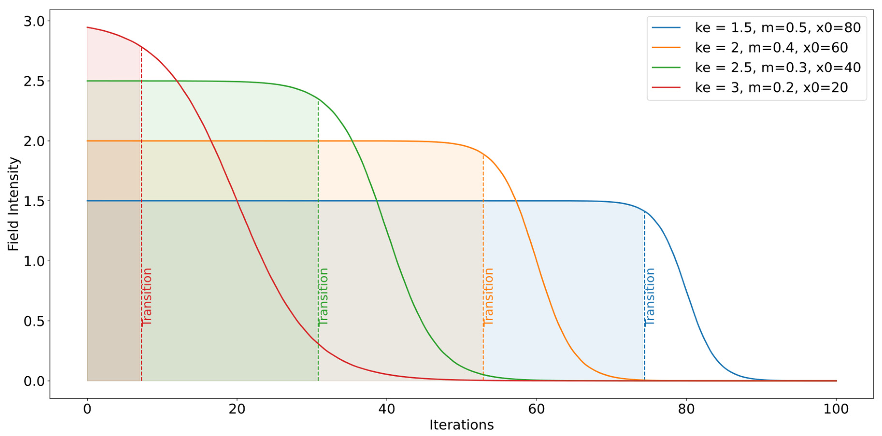
The field intensity (I) dynamically adjusts the storm stages during the optimization process through a logistic function ($\gamma$). This allows for a nonlinear response to variations in field resistance (R), with an imposed decreasing trend influenced by the current iteration (j) relative to the total number of iterations (iter), allowing for the algorithm to adapt its behavior over time, as in Equation (8). This adjustment models three distinct stages of storm development: an initial exploration phase, a transitional phase, and a final exploitation phase. The field intensity is then calculated as the product of $\gamma$ and the field conductivity ($ke$), as in Equation (9).

Figure 2 shows the conceptual behavior of I. The pendent of the curve (m = $\left({\displaystyle \frac{e^{R_j}}{R_j}}\right)$) and the value of the Sigmoid’s midpoint ($x_0=R_j-\left|{\mathit{log}}_e\left(1-{\displaystyle \frac{ic}{iter}}\right)\right|$) are adjusted on the basis of the value of $R$. Consequently, when R is high, $I$ is increased to promote the greater exploration of the search space. Conversely, when $R$ is low, $I$ is decreased to encourage the exploitation of promising areas near the current best solution. This dynamic adjustment of $I$ ensures a balance between exploration and exploitation, maintaining the effectiveness and efficiency of the search process throughout the optimization.

$${\mathit{\gamma }}_{\mathit{j}} = {\displaystyle \frac{\mathbf{1}}{\mathbf{1}+{\mathit{e}}^{\left(-\left(\frac{{\mathit{e}}^{{\mathit{R}}_{\mathit{j}}}}{{\mathit{R}}_{\mathit{j}}}\right)\times \left({\mathit{R}}_{\mathit{j}}-\left|{\mathit{log}}_{\mathit{e}}\left(\mathbf{1}-\frac{\mathit{j}}{\mathit{i}\mathit{t}\mathit{e}\mathit{r}}\right)\right|\right)\right)}}}$$

(8)

$${\mathit{I}}_{\mathit{j}}={\mathit{k}\mathit{e}}_{\mathit{j}}\times {\mathit{\gamma }}_{\mathit{j}}$$

(9)

2.5. Storm Power

Storm power ($P$) plays a crucial role in quantifying the cumulative potential of the search mechanism at any given point during the optimization process. It serves as an adjustment to the intensity of the perturbation introduced to the lightning positions and to the step size for the local search. It is calculated as the product of two dynamically varying factors, $I$ and $R$, as in Equation (10). This definition is inspired by the physical concept of electrical loss, where power loss occurs due to resistance within a system. In the context of the ESO algorithm, this concept is adapted to calculate the remaining power of the storm during the exploration process. This adaptive mechanism ensures that the algorithm remains responsive to the topology of the search space, enabling it to dynamically balance exploration and exploitation on the basis of real-time feedback from the optimization environment.

$${\mathit{P}}_{\mathit{j}}={{\mathit{R}}_{\mathit{j}}\times {\mathit{I}}_{\mathit{j}}}^{{\mathit{k}\mathit{e}}_{\mathit{j}}}$$

(10)

2.6. Lightning Initialization

The initialization process involves strategically positioning new agents either within previously identified promising regions (ionized areas) or randomly within the search space. If ionized areas ($\alpha$) are present ($j>1$), the position of a new lightning event (${\rho }_{i,j}^n$) is determined by selecting a position from $\alpha$ and applying a perturbation equal to the storm power (P) value. If no $\alpha$ is present, the position ${\rho }_{i,j}^n$ is then given by a uniform random distribution within the lower ($b_{low}$) and upper ($b_{high}$) bounds of each dimension, as in Equation (11).

$${\mathit{\rho }}_{\mathit{i},\mathit{j}}^{\mathit{n}}=\left\{\begin{array}{c}U\left({\mathit{b}}_{\mathit{l}\mathit{o}\mathit{w}},{\mathit{b}}_{\mathit{h}\mathit{i}\mathit{g}\mathit{h}}\right),\hspace{1em}\hspace{1em}\mathit{f}\mathit{o}\mathit{r}\hspace{0.17em}\mathit{j}=\mathbf{1}\\ {\alpha }_{\mathit{j}}+{\mathit{P}}_{\mathit{j}}, \mathit{f}\mathit{o}\mathit{r} j \text{>} 1\end{array}\right.$$

(11)

2.7. Branching and Propagation

The ESO algorithm simulates the branching and propagation of lightning via interactions with ionized areas within the search space. The new position of active lightning (${\rho }_{new,j}^n$) is determined on the basis of whether the position of the lightning (${\rho }_{i,j}^n$) is within an ionized area ($\alpha )$ or not. For lightning in $\alpha$, the new position is adjusted by the storm power ($P$), aiming to explore nearby promising areas. For lightning outside of $\alpha$, the new position is influenced by the average position of $\alpha$, scaled by a random uniform perturbation $U\left(-ke,ke\right)$of size ± $ke$ and storm power ($P$), facilitating the exploration of areas with known high-quality solutions, as shown in Equation (12).

$${\mathit{\rho }}_{\mathit{n}\mathit{e}\mathit{w},\mathit{j}}^{\mathit{n}}=\left\{\begin{array}{cc}{\mathit{\rho }}_{\mathit{i},\mathit{j}}^{\mathit{n}}\times {\mathit{P}}_{\mathit{j}}& \mathit{i}\mathit{f} {\mathit{\rho }}_{\mathit{i},\mathit{j}}^{\mathit{n}} \mathit{i}\mathit{n} {\alpha }_{\mathit{j}}\\ {\displaystyle \frac{\mathbf{1}}{{\mathit{N}}_{\alpha }}}{\sum }_{\mathit{i}=\mathbf{1}}^{{\mathit{N}}_{\alpha }}\left({\mathit{\rho }}_{\mathit{i},\mathit{j}}^{\mathit{n}}+\left[\mathit{U}\left(-{\mathit{k}\mathit{e}}_{\mathit{j}},{\mathit{k}\mathit{e}}_{\mathit{j}}\right)\times {\mathit{P}}_{\mathit{j}}\times {\mathit{e}}^{{\mathit{k}\mathit{e}}_{\mathit{j}}}\right]\right),& \mathit{otherwise}\end{array}\right.$$

(12)

2.8. Selection and Evaluation of New Positions

The optimization process seeks to find the optimal solution among complex and vast search spaces. Therefore, an evaluation of the improvements is a critical component of the algorithm, which focuses on the iterative refinement of agent (lightning) positions within the search space. The primary objective of this process is to evaluate new potential positions for each agent and determine whether moving to these new positions would result in an improvement in the fitness of the objective function. This decision-making process is central to the ability of the algorithms to converge on optimal or near-optimal solutions. By systematically comparing the fitness of the function in the new position $f\left({\rho }_{new,j}^n\right)$ with the current best fitness of the function in the best position found thus far ($f\left({\rho }_{best}\right)$), the algorithm decides whether adopting the new path would bring the search closer to the optimization goal, as in Equations (13) and (14). The fitness is obtained by evaluating the objective function in the current coordinates of each lightning strike. Algorithm 1 presents the pseudocode of the main processes in the algorithm.

$$\mathit{u}\mathit{p}\mathit{d}\mathit{a}\mathit{t}\mathit{e}\hspace{0.17em}\mathit{i}\mathit{f}\left\{\begin{array}{c}\mathit{f}\left({\mathit{\rho }}_{\mathit{n}\mathit{e}\mathit{w},\mathit{j}}^{\mathit{n}}\right)<\mathit{f}\left({\mathit{\rho }}_{\mathit{b}\mathit{e}\mathit{s}\mathit{t}}\right), \mathit{f}\mathit{o}\mathit{r} \mathit{m}\mathit{i}\mathit{n}\\ \mathit{f}\left({\mathit{\rho }}_{\mathit{n}\mathit{e}\mathit{w},\mathit{j}}^{\mathit{n}}\right)>\mathit{f}\left({\mathit{\rho }}_{\mathit{b}\mathit{e}\mathit{s}\mathit{t}}\right), \mathit{f}\mathit{o}\mathit{r} \mathit{m}\mathit{a}\mathit{x}\end{array}\right.$$

(13)

$${\mathit{\rho }}_{\mathit{b}\mathit{e}\mathit{s}\mathit{t}}\leftarrow {\mathit{\rho }}_{\mathit{n}\mathit{e}\mathit{w},\mathit{j}}^{\mathit{n}},\hspace{1em}\mathit{f}\left({\mathit{\rho }}_{\mathit{b}\mathit{e}\mathit{s}\mathit{t}}\right)\leftarrow \mathit{f}\left({\mathit{\rho }}_{\mathit{n}\mathit{e}\mathit{w},\mathit{j}}^{\mathit{n}}\right)$$

(14)

Algorithm 1. Pseudocode of the main processes of the electrical storm optimization (ESO) algorithm

3. Results

The effectiveness of the ESO algorithm was assessed through a series of diverse optimization challenges. The evaluation began with 25 primitive unimodal and multimodal problems, testing the efficiency of the ESO in scaping from local optimums and converging to the global optimum. It then proceeded to 20 shifted and rotated problems to explore its ability to navigate multiple local optima in complicated landscapes. Additionally, the ESO faced the IEEE Congress on Evolutionary Computation (CEC) 2022 Single Objective Bound Constrained (SOBC) benchmark set, which includes rotated, shifted, hybrid, and composite functions, showcasing its adaptability to intricate and computationally intensive tasks [43]. The real-world applicability of the algorithm was further validated by its performance on six engineering problems.

The ESO algorithm was benchmarked against 15 of the most cited and utilized metaheuristic algorithms and 5 recently published algorithms, as shown in

Table 1. Overview of 20 metaheuristic algorithms considered for comparison and the default parameters used.

No.	Algorithm (Abbreviation)	Parameters	Reference
1	Artificial Bee Colony (ABC)	n_limits = 50	[51]
2	Ant Colony Optimization (ACO)	Sample_count = 25, intent_factor = 0.5, zeta = 1.0	[52]
3	Ant Lion Optimizer (ALO)	-	[53]
4	Atom Search Optimization (ASO)	alpha = 10, beta = 0.2	[54]
5	Biogeography-Based Optimization (BBO)	p_m = 0.01, n_elites = 2	[55]
6	Brown Bear Optimization Algorithm (BBOA)	-	[23]
7	Differential Evolution (DE)	wf = 0.7, cr = 0.9	[56]
8	Energy Valley Optimizer (EVO)	-	[24]
9	Fick’s Law Algorithm (FLA)	C1 = 0.5, C2 = 2.0, C3 = 0.1, C4 = 0.2, C5 = 2.0, DD = 0.01	[27]
10	Flower Pollination Algorithm (FPA)	p_s = 0.8, levy_mult = 0.2	[57]
11	Genetic Algorithm (GA)	pc = 0.9, pm = 0.05, k_way = 0.4	[58]
12	Gaining Sharing Knowledge-based Algorithm (GSKA)	pb = 0.1, kr = 0.7	[59]
13	Harmony Search (HS)	c_r = 0.95, pa_r = 0.05	[60]
14	Honey Badger Algorithm (HBA)	-	[26]
15	Linear population reduction SHADE (LSHADE)	miu_f = 0.5, miu_cr = 0.5	[61]
16	Moth–Flame Optimization (MFO)	-	[62]
17	Particle Swarm Optimization (PSO)	c1 = 2.05, c2 = 2.05, w = 0.4	[63]
18	Queuing Search Algorithm (QSA)	-	[64]
19	Simulated Annealing (SA)	temp_init = 100, step_size = 0.1	[65]
20	Tabu Search (TS)	-	[66]

[2,7,10,12,32,44,45,46]. Moreover, the comparison set includes the LSHADE algorithm, which was the winner of numerous editions of the IEEE CEC competition [47,48,49,50]. The implementation of the algorithms was retrieved from the Mealpy v30.1 Python library, which is known for its robust and standardized implementations of optimization algorithms, providing a consistent platform for comparative evaluations [8]. To ensure fairness, standard hyperparameters were used, with a population size of 50 and a maximum of 50,000 objective function evaluations. Fifty independent runs were conducted per problem, with no parameter tuning between problems. The default parameters for each algorithm were retrieved from their corresponding papers, as shown in Table 1. However, the comparison focused on the results of the top ten performing algorithms, with the results for the ten lower-performing algorithms detailed in Appendix A 

Table A1. Results of the algorithms with lower performance for the unimodal problems.

		ABC	ACO	ASO	BBOA	BBO	EVO	GA	HBA	SA	TS
F1	Mean	−2.0 × 102	−2.0 × 102	−2.0 × 102	−2.0 × 102	−2.0 × 102	−2.0 × 102	−2.0 × 102	−2.0 × 102	−2.0 × 102	−1.8 × 102
	std	0.0 × 100	0.0 × 100	7.6 × 10−1	0.0 × 100	2.2 × 10−1	1.7 × 100	8.8 × 10−2	0.0 × 100	1.3 × 10−2	6.1 × 100
	Dist.	0.0 × 100	0.0 × 100	9.9 × 10−1	0.0 × 100	3.3 × 10−1	9.0 × 10−1	9.5 × 10−2	0.0 × 100	2.3 × 10−2	1.7 × 101
F2	Mean	0.0 × 100	2.7 × 10−5	2.3 × 10−2	0.0 × 100	3.8 × 10−2	2.1 × 10−1	4.5 × 10−3	0.0 × 100	4.0 × 10−4	7.3 × 100
	std	0.0 × 100	1.2 × 10−4	2.0 × 10−2	0.0 × 100	4.2 × 10−2	4.5 × 10−1	6.8 × 10−3	0.0 × 100	3.5 × 10−4	6.4 × 100
	Dist.	0.0 × 100	2.7 × 10−5	2.3 × 10−2	0.0 × 100	3.8 × 10−2	2.1 × 10−1	4.5 × 10−3	0.0 × 100	4.0 × 10−4	7.3 × 100
F3	Mean	2.0 × 1010	5.7 × 1010	1.7 × 1010	1.8 × 10−118	1.1 × 104	3.3 × 108	8.9 × 108	0.0 × 100	5.2 × 1010	7.1 × 1010
	std	2.5 × 109	3.8 × 109	9.9 × 109	2.2 × 10−118	5.0 × 103	1.5 × 108	1.4 × 108	0.0 × 100	5.6 × 109	6.7 × 109
	Dist.	2.0 × 1010	5.7 × 1010	1.7 × 1010	1.8 × 10−118	1.1 × 104	3.3 × 108	8.9 × 108	0.0 × 100	5.2 × 1010	7.1 × 1010
F4	Mean	1.7 × 100	1.7 × 100	3.1 × 104	1.7 × 100	1.3 × 104	3.7 × 106	1.2 × 102	1.7 × 100	2.7 × 108	5.5 × 109
	std	0.0 × 100	1.1 × 10−2	8.9 × 104	3.1 × 10−16	4.1 × 104	8.6 × 106	2.8 × 102	7.6 × 10−16	7.7 × 108	9.4 × 109
	Dist.	8.0 × 10−5	2.6 × 10−3	3.1 × 104	8.0 × 10−5	1.3 × 104	3.7 × 106	1.2 × 102	8.0 × 10−5	2.7 × 108	5.5 × 109
F5	Mean	2.7 × 10−6	5.0 × 10−2	5.9 × 10−4	0.0 × 100	8.5 × 10−2	2.1 × 10−1	5.7 × 10−2	0.0 × 100	2.2 × 10−3	7.0 × 10−1
	std	3.6 × 10−6	3.1 × 10−2	7.9 × 10−4	0.0 × 100	1.1 × 10−1	2.1 × 10−1	7.9 × 10−2	0.0 × 100	2.6 × 10−3	4.7 × 10−1
	Dist.	2.7 × 10−6	5.0 × 10−2	5.9 × 10−4	0.0 × 100	8.5 × 10−2	2.1 × 10−1	5.7 × 10−2	0.0 × 100	2.2 × 10−3	7.0 × 10−1
F6	Mean	1.0 × 103	1.1 × 103	1.1 × 103	9.8 × 101	1.9 × 102	1.1 × 102	4.7 × 102	9.7 × 101	9.9 × 102	1.6 × 103
	std	4.2 × 101	2.0 × 102	8.3 × 101	1.5 × 10−2	4.5 × 101	1.1 × 101	2.2 × 101	1.9 × 100	6.8 × 101	9.0 × 101
	Dist.	1.0 × 103	1.1 × 103	1.1 × 103	9.8 × 101	1.9 × 102	1.1 × 102	4.7 × 102	9.7 × 101	9.9 × 102	1.6 × 103
F7	Mean	−2.2 × 100	−2.1 × 100	−2.1 × 100	−2.1 × 100	−2.1 × 100	−2.1 × 100	−2.1 × 100	−2.2 × 100	−1.8 × 100	−1.5 × 100
	std	2.7 × 10−16	1.5 × 10−2	4.8 × 10−2	4.6 × 10−2	1.2 × 10−2	9.0 × 10−2	5.0 × 10−3	4.6 × 10−16	2.3 × 10−1	2.5 × 10−1
	Dist.	4.7 × 10−2	5.0 × 10−2	1.2 × 10−1	6.1 × 10−2	7.2 × 10−2	1.2 × 10−1	5.5 × 10−2	4.7 × 10−2	4.1 × 10−1	7.0 × 10−1
F8	Mean	3.1 × 10−15	1.6 × 10−1	3.6 × 10−2	2.5 × 10−31	2.1 × 10−1	9.8 × 100	1.2 × 10−1	1.9 × 10−30	7.4 × 10−2	3.3 × 101
	std	1.5 × 10−14	7.9 × 10−1	3.5 × 10−2	3.7 × 10−31	1.9 × 10−1	1.2 × 101	1.2 × 10−1	4.4 × 10−30	1.6 × 10−1	3.4 × 101
	Dist.	3.1 × 10−15	1.6 × 10−1	3.6 × 10−2	2.5 × 10−31	2.1 × 10−1	9.8 × 100	1.2 × 10−1	1.9 × 10−30	7.4 × 10−2	3.3 × 101
F9	Mean	6.2 × 10−13	9.2 × 10−9	9.0 × 103	0.0 × 100	4.2 × 102	1.2 × 105	1.7 × 100	0.0 × 100	4.8 × 108	2.1 × 109
	std	3.0 × 10−12	3.8 × 10−8	1.6 × 104	0.0 × 100	1.2 × 103	2.8 × 105	4.4 × 100	0.0 × 100	1.2 × 109	3.7 × 109
	Dist.	6.2 × 10−13	9.2 × 10−9	9.0 × 103	0.0 × 100	4.2 × 102	1.2 × 105	1.7 × 100	0.0 × 100	4.8 × 108	2.1 × 109
F10	Mean	−3.5 × 10−1	−3.5 × 10−1	−3.5 × 10−1	−3.5 × 10−1	−3.5 × 10−1	−2.7 × 10−1	−3.5 × 10−1	−3.5 × 10−1	−3.5 × 10−1	7.5 × 10−1
	std	5.6 × 10−17	5.6 × 10−17	7.9 × 10−3	5.6 × 10−17	1.9 × 10−3	8.5 × 10−2	1.3 × 10−4	5.6 × 10−17	9.4 × 10−4	1.5 × 100
	Dist.	8.6 × 10−5	8.6 × 10−5	4.4 × 10−3	8.6 × 10−5	1.3 × 10−3	8.5 × 10−2	3.3 × 10−5	8.6 × 10−5	4.9 × 10−4	1.1 × 100
F11	Mean	−2.0 × 100	−2.0 × 100	−2.0 × 100	−2.0 × 100	−2.0 × 100	−2.0 × 100	−2.0 × 100	−2.0 × 100	−1.5 × 101	−1.8 × 100
	std	0.0 × 100	0.0 × 100	2.1 × 10−3	0.0 × 100	7.3 × 10−3	7.1 × 10−4	1.6 × 10−3	0.0 × 100	3.5 × 100	1.7 × 10−1
	Dist.	6.8 × 10−6	6.8 × 10−6	2.7 × 10−3	6.8 × 10−6	5.8 × 10−3	2.7 × 10−4	1.3 × 10−3	6.8 × 10−6	1.3 × 101	2.2 × 10−1
F12	Mean	4.0 × 10−1	4.0 × 10−1	4.0 × 10−1	4.0 × 10−1	4.0 × 10−1	4.9 × 10−1	4.0 × 10−1	4.0 × 10−1	4.0 × 10−1	1.5 × 100
	std	0.0 × 100	0.0 × 100	6.8 × 10−3	0.0 × 100	3.0 × 10−3	1.6 × 10−1	7.7 × 10−4	0.0 × 100	2.6 × 10−4	10.0 × 10−1
	Dist.	7.4 × 10−6	7.4 × 10−6	5.0 × 10−3	7.4 × 10−6	2.7 × 10−3	9.5 × 10−2	4.7 × 10−4	7.4 × 10−6	2.3 × 10−4	1.1 × 100
F13	Mean	2.7 × 10−2	4.9 × 10−1	4.5 × 10−1	2.7 × 10−3	4.3 × 10−1	2.0 × 10−1	3.3 × 10−1	8.0 × 10−4	5.0 × 10−1	9.2 × 10−1
	std	4.8 × 10−2	5.8 × 10−2	7.2 × 10−2	6.7 × 10−3	6.1 × 10−2	1.5 × 10−1	5.0 × 10−2	5.3 × 10−4	9.7 × 10−2	1.3 × 10−1
	Dist.	2.7 × 10−2	4.9 × 10−1	4.5 × 10−1	2.6 × 10−3	4.3 × 10−1	2.0 × 10−1	3.3 × 10−1	7.0 × 10−4	5.0 × 10−1	9.2 × 10−1
F14	Mean	−7.2 × 10−4	−2.1 × 10−4	−2.3 × 10−4	−2.0 × 10−1	−2.5 × 10−4	−8.9 × 10−4	−3.0 × 10−4	−2.7 × 10−1	−1.6 × 10−4	−1.1 × 10−4
	std	3.1 × 10−4	4.1 × 10−5	2.8 × 10−5	3.5 × 10−1	7.2 × 10−5	1.5 × 10−3	4.1 × 10−5	3.7 × 10−1	2.4 × 10−5	1.5 × 10−5
	Dist.	10.0 × 10−1	10.0 × 10−1	10.0 × 10−1	8.0 × 10−1	10.0 × 10−1	10.0 × 10−1	10.0 × 10−1	7.3 × 10−1	10.0 × 10−1	10.0 × 10−1
F15	Mean	−2.1 × 100	−2.1 × 100	−2.1 × 100	−2.1 × 100	−2.1 × 100	−2.1 × 100	−2.1 × 100	−2.1 × 100	−2.0 × 100	−2.0 × 100
	std	0.0 × 100	1.6 × 10−8	2.8 × 10−4	0.0 × 100	4.5 × 10−5	4.4 × 10−4	2.0 × 10−6	0.0 × 100	5.0 × 10−2	7.0 × 10−2
	Dist.	1.2 × 10−5	1.2 × 10−5	1.5 × 10−4	1.2 × 10−5	2.1 × 10−5	3.4 × 10−4	1.0 × 10−5	1.2 × 10−5	2.0 × 10−2	6.6 × 10−2
F16	Mean	2.0 × 100	2.0 × 100	1.9 × 100	1.9 × 100	2.0 × 100	2.0 × 100	2.0 × 100	−8.9 × 10−14	2.0 × 100	4.0 × 100
	std	2.9 × 10−2	0.0 × 100	3.6 × 10−1	3.9 × 10−1	8.1 × 10−4	2.9 × 10−2	6.2 × 10−5	1.7 × 10−14	1.7 × 10−4	1.9 × 100
	Dist.	2.0 × 100	2.0 × 100	1.9 × 100	1.9 × 100	2.0 × 100	2.0 × 100	2.0 × 100	8.9 × 10−14	2.0 × 100	4.0 × 100
F17	Mean	2.9 × 10−3	5.9 × 10−3	2.0 × 10−2	8.9 × 10−6	6.6 × 10−3	2.2 × 10−2	3.1 × 10−3	5.3 × 10−4	6.0 × 10−3	1.4 × 101
	std	2.4 × 10−3	4.9 × 10−3	2.8 × 10−2	2.3 × 10−5	6.9 × 10−3	9.0 × 10−2	3.0 × 10−3	1.2 × 10−3	7.8 × 10−3	1.4 × 101
	Dist.	2.9 × 10−3	5.9 × 10−3	2.0 × 10−2	8.9 × 10−6	6.6 × 10−3	2.2 × 10−2	3.1 × 10−3	5.3 × 10−4	6.0 × 10−3	1.4 × 101
F18	Mean	−1.0 × 100	−1.0 × 100	−5.0 × 10−1	−1.0 × 100	−3.7 × 10−1	−6.5 × 10−1	−5.6 × 10−1	−1.0 × 100	−4.0 × 10−2	−7.0 × 10−7
	std	0.0 × 100	0.0 × 100	3.6 × 10−1	0.0 × 100	4.3 × 10−1	4.7 × 10−1	4.8 × 10−1	0.0 × 100	2.0 × 10−1	3.4 × 10−6
	Dist.	0.0 × 100	0.0 × 100	5.0 × 10−1	0.0 × 100	6.3 × 10−1	3.5 × 10−1	4.4 × 10−1	0.0 × 100	9.6 × 10−1	10.0 × 10−1
F19	Mean	3.0 × 100	3.0 × 100	3.1 × 100	3.0 × 100	7.1 × 100	9.4 × 100	3.0 × 100	1.1 × 101	1.5 × 101	3.6 × 101
	std	1.1 × 10−15	1.6 × 10−2	9.5 × 10−2	6.6 × 10−16	9.9 × 100	9.1 × 100	1.6 × 10−3	2.2 × 101	1.9 × 101	3.5 × 101
	Dist.	7.8 × 10−14	3.2 × 10−3	8.5 × 10−2	7.9 × 10−14	4.1 × 100	6.4 × 100	1.4 × 10−3	7.6 × 100	1.2 × 101	3.3 × 101
F20	Mean	−1.9 × 101	−1.9 × 101	−1.9 × 101	−1.9 × 101	−1.9 × 101	−1.9 × 101	−1.9 × 101	−1.9 × 101	−1.7 × 101	−1.4 × 101
	std	0.0 × 100	7.4 × 10−3	1.4 × 10−2	3.0 × 10−15	2.0 × 10−3	9.3 × 10−2	3.3 × 10−4	3.7 × 10−15	3.9 × 100	3.6 × 100
	Dist.	5.0 × 10−4	1.8 × 10−3	1.2 × 10−2	5.0 × 10−4	1.6 × 10−3	4.2 × 10−2	3.6 × 10−4	5.0 × 10−4	2.4 × 100	5.1 × 100
F21	Mean	−2.5 × 100	−2.3 × 100	−2.1 × 100	−3.0 × 100	−2.8 × 100	−2.8 × 100	−3.0 × 100	−3.0 × 100	−1.2 × 100	−6.5 × 10−1
	std	2.2 × 10−1	4.8 × 10−1	4.5 × 10−1	0.0 × 100	3.7 × 10−1	3.8 × 10−1	1.8 × 10−1	3.4 × 10−6	6.8 × 10−1	2.8 × 10−1
	Dist.	4.6 × 10−1	7.1 × 10−1	9.0 × 10−1	0.0 × 100	1.9 × 10−1	2.5 × 10−1	3.7 × 10−2	1.1 × 10−6	1.8 × 100	2.4 × 100
F22	Mean	2.0 × 100	2.0 × 100	5.7 × 100	3.4 × 100	2.0 × 100	7.0 × 100	2.0 × 100	2.7 × 100	1.0 × 100	4.3 × 102
	std	0.0 × 100	0.0 × 100	1.8 × 100	4.2 × 100	1.4 × 10−2	3.5 × 100	4.8 × 10−3	1.9 × 100	2.3 × 10−6	3.3 × 102
	Dist.	0.0 × 100	0.0 × 100	3.7 × 100	1.4 × 100	4.4 × 10−2	5.0 × 100	1.5 × 10−2	7.2 × 10−1	10.0 × 10−1	4.2 × 102
F23	Mean	−3.3 × 10−66	−4.9 × 10−71	−2.6 × 10−55	−4.6 × 10−3	−2.3 × 10−84	−8.7 × 10−3	−4.3 × 10−60	−8.5 × 10−3	−1.5 × 10−105	−9.4 × 10−176
	std	1.6 × 10−65	2.4 × 10−70	1.3 × 10−54	4.6 × 10−3	1.1 × 10−83	4.0 × 10−2	2.1 × 10−59	7.3 × 10−3	7.4 × 10−105	0.0 × 100
	Dist.	1.0 × 100	1.0 × 100	1.0 × 100	1.0 × 100	1.0 × 100	10.0 × 10−1	1.0 × 100	10.0 × 10−1	1.0 × 100	1.0 × 100
F24	Mean	10.0 × 10−1	1.0 × 100	10.0 × 10−1	1.0 × 100	1.0 × 100	1.0 × 100	1.0 × 100	9.6 × 10−1	1.0 × 100	1.1 × 100
	std	3.4 × 10−3	2.8 × 10−4	1.3 × 10−2	4.5 × 10−5	2.3 × 10−5	1.3 × 10−3	1.3 × 10−6	4.9 × 10−2	3.3 × 10−4	7.6 × 10−2
	Dist.	9.9 × 10−2	1.0 × 10−1	9.7 × 10−2	1.0 × 10−1	1.0 × 10−1	1.0 × 10−1	1.0 × 10−1	6.0 × 10−2	1.0 × 10−1	1.6 × 10−1
F25	Mean	3.9 × 101	6.5 × 101	3.5 × 101	5.3 × 101	6.3 × 101	6.8 × 101	5.5 × 101	3.4 × 101	7.1 × 101	7.5 × 101
	std	7.0 × 100	1.2 × 101	2.4 × 100	2.0 × 101	1.8 × 101	1.3 × 101	2.0 × 101	2.6 × 10−14	1.1 × 101	6.1 × 100
	Dist.	4.1 × 100	3.0 × 101	1.1 × 100	1.9 × 101	2.9 × 101	3.3 × 101	2.1 × 101	3.3 × 10−1	3.6 × 101	4.0 × 101

,

Table A2. Results of the algorithms with lower performance for multimodal problems.

		ABC	ACO	ASO	BBOA	BBO	EVO	GA	HBA	SA	TS
F26	Mean	7.7 × 100	1.3 × 101	1.9 × 101	8.6 × 100	5.8 × 100	5.7 × 100	4.0 × 100	7.5 × 100	2.0 × 101	2.1 × 101
	std	1.2 × 100	6.9 × 10−1	2.8 × 10−1	3.4 × 10−1	8.5 × 10−1	9.3 × 10−1	2.9 × 10−1	4.8 × 10−1	2.8 × 10−1	3.2 × 10−1
	Dist.	7.7 × 100	1.3 × 101	1.9 × 101	8.6 × 100	5.8 × 100	5.7 × 100	4.0 × 100	7.5 × 100	2.0 × 101	2.1 × 101
F27	Mean	3.6 × 101	4.1 × 101	4.1 × 101	1.4 × 101	9.8 × 100	1.3 × 101	5.3 × 100	9.3 × 100	1.5 × 101	6.3 × 101
	std	1.6 × 100	2.9 × 100	4.1 × 100	1.4 × 100	2.1 × 100	2.7 × 100	1.4 × 100	2.4 × 100	2.9 × 100	6.5 × 100
	Dist.	3.6 × 101	4.1 × 101	4.1 × 101	1.4 × 101	9.8 × 100	1.3 × 101	5.3 × 100	9.3 × 100	1.5 × 101	6.3 × 101
F28	Mean	1.9 × 102	5.5 × 102	1.3 × 103	8.9 × 102	2.1 × 100	2.5 × 102	8.2 × 100	7.3 × 101	3.8 × 101	3.3 × 103
	std	3.1 × 101	9.1 × 101	2.0 × 102	1.4 × 102	4.6 × 10−1	7.7 × 101	2.7 × 100	4.3 × 101	1.4 × 101	5.1 × 102
	Dist.	1.9 × 102	5.5 × 102	1.3 × 103	8.9 × 102	2.1 × 100	2.5 × 102	8.2 × 100	7.3 × 101	3.8 × 101	3.3 × 103
F29	Mean	9.4 × 10−2	9.7 × 10−1	2.7 × 102	3.2 × 100	4.8 × 10−3	7.8 × 101	9.8 × 10−2	7.3 × 10−1	1.3 × 100	8.5 × 105
	std	5.2 × 10−2	1.2 × 10−1	8.0 × 101	5.0 × 10−1	1.1 × 10−3	3.5 × 101	2.7 × 10−2	2.3 × 10−1	3.2 × 10−1	1.2 × 106
	Dist.	9.4 × 10−2	9.7 × 10−1	2.7 × 102	3.2 × 100	4.8 × 10−3	7.8 × 101	9.8 × 10−2	7.3 × 10−1	1.3 × 100	8.5 × 105
F30	Mean	3.8 × 10−2	7.9 × 10−1	4.7 × 101	7.7 × 10−3	1.5 × 10−7	4.6 × 10−2	3.1 × 10−6	8.8 × 10−5	1.5 × 10−1	3.3 × 102
	std	3.5 × 10−2	3.0 × 10−1	2.6 × 101	3.5 × 10−3	1.9 × 10−7	2.6 × 10−2	1.4 × 10−6	7.7 × 10−5	4.1 × 10−2	9.6 × 101
	Dist.	3.8 × 10−2	7.9 × 10−1	4.7 × 101	7.7 × 10−3	1.5 × 10−7	4.6 × 10−2	3.1 × 10−6	8.8 × 10−5	1.5 × 10−1	3.3 × 102
F31	Mean	1.3 × 103	1.1 × 107	9.7 × 108	5.9 × 106	3.3 × 101	1.6 × 107	4.4 × 103	5.3 × 105	2.4 × 109	5.3 × 109
	std	10.0 × 102	3.8 × 106	3.3 × 108	3.0 × 106	3.4 × 101	1.1 × 107	1.5 × 103	5.2 × 105	5.1 × 108	6.7 × 108
	Dist.	1.3 × 103	1.1 × 107	9.7 × 108	5.9 × 106	3.3 × 101	1.6 × 107	4.4 × 103	5.3 × 105	2.4 × 109	5.3 × 109
F32	Mean	1.2 × 103	1.2 × 104	5.3 × 105	3.3 × 103	1.3 × 101	6.2 × 103	2.9 × 101	8.9 × 101	1.5 × 102	2.0 × 106
	std	1.2 × 103	5.9 × 103	2.0 × 105	1.4 × 103	1.6 × 101	4.3 × 103	1.1 × 101	5.3 × 101	1.4 × 102	3.5 × 105
	Dist.	1.2 × 103	1.2 × 104	5.3 × 105	3.3 × 103	1.3 × 101	6.2 × 103	2.9 × 101	8.9 × 101	1.5 × 102	2.0 × 106
F33	Mean	1.5 × 10−2	2.9 × 10−2	2.2 × 10−2	3.1 × 10−4	4.2 × 10−2	4.1 × 10−2	6.8 × 10−3	7.0 × 10−2	3.7 × 100	1.5 × 101
	std	8.2 × 10−3	2.3 × 10−2	1.9 × 10−2	9.1 × 10−4	3.4 × 10−2	3.0 × 10−2	4.4 × 10−3	2.0 × 10−1	7.0 × 100	8.2 × 100
	Dist.	1.5 × 10−2	2.9 × 10−2	2.2 × 10−2	3.1 × 10−4	4.2 × 10−2	4.1 × 10−2	6.8 × 10−3	7.0 × 10−2	3.7 × 100	1.5 × 101
F34	Mean	2.4 × 106	1.1 × 109	1.0 × 109	4.2 × 105	2.2 × 10−2	5.5 × 106	1.1 × 10−2	5.9 × 100	8.1 × 100	2.2 × 1014
	std	3.0 × 106	1.0 × 109	1.4 × 109	1.2 × 106	9.2 × 10−3	1.5 × 107	6.8 × 10−3	1.0 × 101	7.9 × 100	4.2 × 1014
	Dist.	2.4 × 106	1.1 × 109	1.0 × 109	4.2 × 105	2.2 × 10−2	5.5 × 106	1.1 × 10−2	5.9 × 100	8.1 × 100	2.2 × 1014
F35	Mean	8.1 × 104	3.7 × 106	2.6 × 108	8.2 × 104	1.9 × 101	7.3 × 105	7.3 × 100	8.9 × 101	2.1 × 108	1.3 × 109
	std	8.7 × 104	1.7 × 106	9.2 × 107	8.6 × 104	2.0 × 101	5.9 × 105	4.8 × 100	4.0 × 101	8.0 × 107	2.7 × 108
	Dist.	8.1 × 104	3.7 × 106	2.6 × 108	8.2 × 104	1.9 × 101	7.3 × 105	7.3 × 100	8.9 × 101	2.1 × 108	1.3 × 109
F36	Mean	3.1 × 10−1	1.0 × 100	4.1 × 101	2.4 × 100	1.2 × 10−1	1.2 × 100	6.3 × 10−2	4.7 × 10−1	8.9 × 10−1	1.7 × 102
	std	6.9 × 10−2	2.9 × 10−1	1.3 × 101	1.2 × 100	6.6 × 10−2	6.9 × 10−1	1.7 × 10−2	2.0 × 10−1	3.7 × 10−1	3.5 × 101
	Dist.	3.1 × 10−1	1.0 × 100	4.1 × 101	2.4 × 100	1.2 × 10−1	1.2 × 100	6.3 × 10−2	4.7 × 10−1	8.9 × 10−1	1.7 × 102
F37	Mean	−2.1 × 100	−1.9 × 100	−1.5 × 100	−1.5 × 100	−1.4 × 100	−1.5 × 100	−1.2 × 100	−2.0 × 100	−1.5 × 100	−1.1 × 100
	std	3.4 × 10−2	3.7 × 10−1	3.3 × 10−1	4.5 × 10−1	3.9 × 10−1	4.6 × 10−1	2.0 × 10−12	1.6 × 10−1	3.0 × 10−1	1.0 × 10−1
	Dist.	2.1 × 100	1.9 × 100	1.5 × 100	1.5 × 100	1.4 × 100	1.5 × 100	1.2 × 100	2.0 × 100	1.5 × 100	1.1 × 100
F38	Mean	4.5 × 101	4.4 × 101	6.9 × 101	3.8 × 101	2.0 × 101	2.9 × 101	9.9 × 100	2.9 × 101	9.3 × 101	1.0 × 102
	std	3.2 × 100	4.8 × 100	6.1 × 100	2.9 × 100	6.7 × 100	6.2 × 100	3.4 × 100	4.5 × 100	9.0 × 100	5.4 × 100
	Dist.	4.7 × 101	4.6 × 101	7.1 × 101	4.0 × 101	2.2 × 101	3.1 × 101	1.2 × 101	3.2 × 101	9.6 × 101	1.0 × 102
F39	Mean	3.9 × 101	3.1 × 103	3.4 × 104	2.2 × 103	3.9 × 100	3.0 × 103	6.1 × 101	5.4 × 102	4.5 × 104	6.5 × 104
	std	2.7 × 101	5.8 × 102	4.7 × 103	2.1 × 102	1.6 × 100	9.8 × 102	1.2 × 101	2.3 × 102	8.0 × 103	9.7 × 103
	Dist.	3.9 × 101	3.1 × 103	3.4 × 104	2.2 × 103	3.9 × 100	3.0 × 103	6.1 × 101	5.4 × 102	4.5 × 104	6.5 × 104
F40	Mean	6.7 × 101	3.5 × 103	3.1 × 104	3.9 × 103	2.4 × 101	3.1 × 103	8.4 × 101	1.6 × 103	6.3 × 104	6.6 × 104
	std	3.3 × 101	6.8 × 102	6.0 × 103	8.0 × 102	7.1 × 100	8.3 × 102	2.1 × 101	4.9 × 102	5.7 × 103	9.7 × 103
	Dist.	6.7 × 101	3.5 × 103	3.1 × 104	3.9 × 103	2.4 × 101	3.1 × 103	8.4 × 101	1.6 × 103	6.3 × 104	6.6 × 104
F41	Mean	6.0 × 100	7.4 × 100	1.9 × 101	5.3 × 100	1.8 × 100	5.2 × 100	2.4 × 100	3.9 × 100	2.5 × 101	2.7 × 101
	std	4.2 × 10−1	6.6 × 10−1	1.4 × 100	5.1 × 10−1	2.1 × 10−1	5.9 × 10−1	2.8 × 10−1	4.6 × 10−1	2.0 × 100	1.7 × 100
	Dist.	6.0 × 100	7.4 × 100	1.9 × 101	5.3 × 100	1.8 × 100	5.2 × 100	2.4 × 100	3.9 × 100	2.5 × 101	2.7 × 101
F42	Mean	5.0 × 10−1	5.0 × 10−1	5.0 × 10−1	4.6 × 10−1	1.4 × 10−1	2.7 × 10−1	2.9 × 10−1	3.3 × 10−1	5.0 × 10−1	5.0 × 10−1
	std	1.5 × 10−4	3.5 × 10−4	9.1 × 10−5	1.1 × 10−2	4.3 × 10−2	1.8 × 10−1	7.2 × 10−2	7.4 × 10−2	2.0 × 10−5	1.4 × 10−5
	Dist.	5.0 × 10−1	5.0 × 10−1	5.0 × 10−1	4.6 × 10−1	1.4 × 10−1	2.7 × 10−1	2.9 × 10−1	3.3 × 10−1	5.0 × 10−1	5.0 × 10−1
F43	Mean	3.0 × 10−6	5.8 × 10−6	1.1 × 10−6	2.1 × 10−8	9.0 × 10−10	2.8 × 10−5	4.0 × 10−10	7.9 × 10−9	1.7 × 10−5	3.4 × 10−3
	std	2.0 × 10−6	4.3 × 10−6	5.1 × 10−7	1.8 × 10−8	1.1 × 10−9	4.9 × 10−5	3.2 × 10−10	1.9 × 10−8	1.0 × 10−5	3.2 × 10−3
	Dist.	3.0 × 10−6	5.8 × 10−6	1.1 × 10−6	2.1 × 10−8	9.0 × 10−10	2.8 × 10−5	4.0 × 10−10	7.9 × 10−9	1.7 × 10−5	3.4 × 10−3
F44	Mean	6.9 × 102	8.9 × 102	4.9 × 102	8.2 × 101	3.1 × 102	5.6 × 102	5.0 × 102	1.6 × 101	6.6 × 102	5.8 × 103
	std	6.1 × 101	8.3 × 101	7.5 × 101	9.0 × 100	1.1 × 102	1.7 × 102	9.5 × 101	7.1 × 100	1.5 × 102	7.2 × 103
	Dist.	6.9 × 102	8.9 × 102	4.9 × 102	8.2 × 101	3.1 × 102	5.6 × 102	5.0 × 102	1.6 × 101	6.6 × 102	5.8 × 103
F45	Mean	2.8 × 100	5.0 × 100	3.9 × 100	0.0 × 100	2.4 × 100	2.5 × 100	2.5 × 100	1.9 × 100	3.5 × 100	7.5 × 101
	std	8.9 × 10−1	1.7 × 100	1.5 × 100	0.0 × 100	6.2 × 10−1	1.6 × 100	9.4 × 10−1	4.6 × 10−1	1.3 × 100	3.3 × 101
	Dist.	2.8 × 100	5.0 × 100	3.9 × 100	0.0 × 100	2.4 × 100	2.5 × 100	2.5 × 100	1.9 × 100	3.5 × 100	7.5 × 101

and

Table A3. Results of the algorithms with lower performance for the CEC 2022 problems.

		ABC	ACO	ASO	BBOA	BBO	EVO	GA	HBA	SA	TS
D = 10
F46	Mean	3.0 × 102	3.0 × 102	5.5 × 103	3.2 × 103	4.0 × 102	5.9 × 103	3.0 × 102	3.0 × 102	1.5 × 104	3.1 × 104
	std	3.0 × 10−10	2.4 × 10−3	1.8 × 103	1.8 × 103	1.5 × 102	3.2 × 103	1.1 × 100	1.4 × 10−2	6.6 × 103	9.8 × 103
	Dist.	1.1 × 10−10	1.4 × 10−3	5.2 × 103	2.9 × 103	1.0 × 102	5.6 × 103	9.3 × 10−1	1.5 × 10−2	1.5 × 104	3.1 × 104
F47	Mean	4.1 × 102	4.1 × 102	5.9 × 102	6.4 × 102	4.1 × 102	5.3 × 102	4.1 × 102	4.1 × 102	1.3 × 103	3.1 × 103
	std	2.7 × 10−1	6.6 × 10−1	5.4 × 101	1.7 × 102	1.7 × 101	9.0 × 101	2.1 × 101	2.2 × 101	5.7 × 102	1.0 × 103
	Dist.	8.9 × 100	8.6 × 100	1.9 × 102	2.4 × 102	1.1 × 101	1.3 × 102	1.4 × 101	1.4 × 101	9.3 × 102	2.7 × 103
F48	Mean	6.0 × 102	6.0 × 102	6.0 × 102	6.0 × 102	6.0 × 102	6.0 × 102	6.0 × 102	6.0 × 102	6.0 × 102	6.0 × 102
	std	0.0 × 100	0.0 × 100	4.4 × 10−2	7.4 × 10−2	3.0 × 10−5	2.8 × 10−2	3.7 × 10−6	6.6 × 10−7	2.2 × 10−1	2.5 × 10−1
	Dist.	0.0 × 100	0.0 × 100	1.5 × 10−1	1.6 × 10−1	4.3 × 10−5	5.0 × 10−2	5.3 × 10−6	1.1 × 10−6	8.6 × 10−1	8.8 × 10−1
F49	Mean	8.5 × 102	8.5 × 102	8.8 × 102	8.3 × 102	8.5 × 102	8.6 × 102	8.5 × 102	8.4 × 102	9.6 × 102	1.0 × 103
	std	8.2 × 100	1.2 × 101	1.4 × 101	8.6 × 100	2.5 × 101	2.7 × 101	2.2 × 101	1.6 × 101	4.6 × 101	3.7 × 101
	Dist.	4.6 × 101	5.2 × 101	7.9 × 101	2.7 × 101	5.5 × 101	6.3 × 101	4.7 × 101	4.0 × 101	1.6 × 102	2.2 × 102
F50	Mean	9.0 × 102	9.0 × 102	9.0 × 102	9.0 × 102	9.0 × 102	9.0 × 102	9.0 × 102	9.0 × 102	9.1 × 102	9.1 × 102
	std	1.9 × 10−8	6.7 × 10−9	7.2 × 10−1	5.2 × 10−1	2.5 × 10−1	4.1 × 10−1	3.0 × 10−1	5.6 × 10−1	2.3 × 100	3.3 × 100
	Dist.	8.0 × 10−9	5.5 × 10−9	1.8 × 100	8.3 × 10−1	2.9 × 10−1	6.7 × 10−1	3.0 × 10−1	6.4 × 10−1	7.5 × 100	10.0 × 100
F51	Mean	5.0 × 104	6.9 × 104	1.4 × 107	2.5 × 104	1.1 × 105	6.9 × 106	2.9 × 104	1.8 × 104	3.1 × 107	1.3 × 109
	std	1.1 × 104	4.9 × 104	1.7 × 107	1.8 × 104	2.0 × 105	1.2 × 107	1.8 × 104	1.2 × 104	9.8 × 107	9.0 × 108
	Dist.	4.9 × 104	6.8 × 104	1.4 × 107	2.4 × 104	1.1 × 105	6.9 × 106	2.7 × 104	1.6 × 104	3.1 × 107	1.3 × 109
F52	Mean	2.0 × 103	2.1 × 103	2.2 × 103	2.0 × 103	2.0 × 103	2.1 × 103	2.0 × 103	2.0 × 103	3.6 × 103	4.6 × 103
	std	6.3 × 100	1.0 × 101	9.2 × 101	1.6 × 101	6.8 × 100	8.6 × 101	7.1 × 100	1.1 × 101	6.1 × 102	1.2 × 103
	Dist.	4.5 × 101	6.2 × 101	2.2 × 102	3.9 × 101	2.6 × 101	1.1 × 102	2.0 × 101	3.2 × 101	1.6 × 103	2.6 × 103
F53	Mean	2.2 × 103	2.3 × 103	8.0 × 103	2.2 × 103	2.6 × 103	3.4 × 107	2.6 × 103	2.2 × 103	4.5 × 103	6.7 × 1013
	std	4.7 × 100	1.4 × 102	2.0 × 104	2.0 × 101	5.6 × 102	1.5 × 108	5.5 × 102	1.9 × 101	1.4 × 103	2.6 × 1014
	Dist.	3.5 × 101	1.3 × 102	5.8 × 103	3.4 × 101	4.2 × 102	3.4 × 107	3.8 × 102	3.4 × 101	2.3 × 103	6.7 × 1013
F54	Mean	2.6 × 103	2.7 × 103	2.8 × 103	2.7 × 103	2.6 × 103	2.7 × 103	2.5 × 103	2.6 × 103	3.3 × 103	3.8 × 103
	std	9.6 × 101	1.0 × 100	1.2 × 102	2.2 × 102	1.7 × 102	1.6 × 102	1.8 × 102	1.6 × 102	2.7 × 102	4.5 × 102
	Dist.	2.7 × 102	3.7 × 102	4.7 × 102	3.7 × 102	2.8 × 102	4.3 × 102	2.4 × 102	2.6 × 102	9.6 × 102	1.5 × 103
F55	Mean	1.7 × 103	2.3 × 103	2.1 × 103	2.0 × 103	1.4 × 103	2.1 × 103	7.8 × 102	6.5 × 102	2.3 × 103	3.4 × 103
	std	3.0 × 102	3.0 × 102	2.8 × 102	6.7 × 102	6.8 × 102	7.0 × 102	5.9 × 102	5.8 × 102	5.0 × 102	4.8 × 102
	Dist.	6.8 × 102	1.4 × 102	3.4 × 102	3.8 × 102	1.0 × 103	2.9 × 102	1.6 × 103	1.7 × 103	1.1 × 102	1.0 × 103
F56	Mean	2.6 × 103	3.2 × 103	2.7 × 103	2.7 × 103	2.6 × 103	2.8 × 103	2.6 × 103	2.6 × 103	3.2 × 103	5.0 × 103
	std	1.5 × 10−6	2.6 × 102	4.9 × 101	7.7 × 101	1.7 × 102	2.5 × 102	7.8 × 100	7.7 × 102	6.3 × 102	1.1 × 103
	Dist.	4.9 × 10−7	5.6 × 102	9.1 × 101	9.1 × 101	3.9 × 101	1.6 × 102	4.1 × 100	3.0 × 101	6.1 × 102	2.4 × 103
F57	Mean	2.9 × 103	2.9 × 103	2.9 × 103	2.9 × 103	2.7 × 103	2.9 × 103	2.4 × 103	2.8 × 103	3.1 × 103	3.4 × 103
	std	2.1 × 100	1.3 × 100	5.2 × 101	3.5 × 101	2.0 × 102	2.3 × 101	3.3 × 102	5.9 × 101	9.8 × 101	2.1 × 102
	Dist.	1.6 × 102	1.6 × 102	1.9 × 102	1.9 × 102	2.7 × 101	1.9 × 102	3.0 × 102	1.5 × 102	3.8 × 102	6.8 × 102
D = 20
F46	Mean	1.1 × 104	6.9 × 103	2.5 × 104	2.1 × 104	1.3 × 103	2.4 × 104	5.1 × 102	6.9 × 102	6.0 × 104	8.7 × 104
	std	1.8 × 103	1.5 × 103	5.8 × 103	5.1 × 103	9.0 × 102	1.0 × 104	2.6 × 102	7.5 × 102	1.5 × 104	4.3 × 104
	Dist.	1.0 × 104	6.6 × 103	2.5 × 104	2.1 × 104	1.0 × 103	2.4 × 104	2.1 × 102	3.9 × 102	5.9 × 104	8.6 × 104
F47	Mean	4.5 × 102	4.5 × 102	1.9 × 103	1.6 × 103	4.7 × 102	7.8 × 102	4.6 × 102	5.1 × 102	4.5 × 103	8.5 × 103
	std	9.3 × 10−2	2.9 × 10−1	3.9 × 102	4.9 × 102	3.2 × 101	1.3 × 102	1.4 × 101	6.5 × 101	1.3 × 103	2.1 × 103
	Dist.	4.9 × 101	5.0 × 101	1.5 × 103	1.2 × 103	6.5 × 101	3.8 × 102	5.9 × 101	1.1 × 102	4.1 × 103	8.1 × 103
F48	Mean	6.0 × 102	6.0 × 102	6.0 × 102	6.0 × 102	6.0 × 102	6.0 × 102	6.0 × 102	6.0 × 102	6.0 × 102	6.0 × 102
	std	3.8 × 10−10	3.7 × 10−5	2.9 × 10−1	2.9 × 10−1	5.8 × 10−5	1.2 × 10−1	2.0 × 10−5	5.6 × 10−2	4.3 × 10−1	4.6 × 10−1
	Dist.	6.0 × 10−10	1.4 × 10−4	1.1 × 100	1.5 × 100	1.3 × 10−4	2.9 × 10−1	5.0 × 10−5	3.4 × 10−2	2.8 × 100	2.9 × 100
F49	Mean	1.0 × 103	1.0 × 103	1.1 × 103	9.6 × 102	9.3 × 102	1.0 × 103	8.8 × 102	9.6 × 102	1.2 × 103	1.4 × 103
	std	2.9 × 101	2.6 × 101	3.6 × 101	2.6 × 101	3.5 × 101	6.6 × 101	2.1 × 101	4.4 × 101	6.4 × 101	6.7 × 101
	Dist.	2.4 × 102	2.3 × 102	3.2 × 102	1.6 × 102	1.3 × 102	2.1 × 102	8.5 × 101	1.6 × 102	4.3 × 102	5.8 × 102
F50	Mean	9.0 × 102	9.0 × 102	9.1 × 102	9.1 × 102	9.0 × 102	9.0 × 102	9.0 × 102	9.0 × 102	9.2 × 102	9.4 × 102
	std	2.1 × 10−1	7.1 × 10−2	2.5 × 100	1.6 × 100	9.4 × 10−1	1.4 × 100	6.4 × 10−1	1.6 × 100	4.6 × 100	8.7 × 100
	Dist.	3.7 × 10−1	5.0 × 10−1	1.0 × 101	5.4 × 100	1.3 × 100	3.6 × 100	1.3 × 100	3.3 × 100	2.4 × 101	3.6 × 101
F51	Mean	9.4 × 107	1.9 × 108	1.4 × 109	9.3 × 108	2.7 × 105	7.9 × 107	1.4 × 105	9.5 × 104	3.3 × 109	8.8 × 109
	std	2.6 × 107	9.8 × 107	5.9 × 108	8.8 × 108	1.7 × 105	1.1 × 108	5.5 × 104	3.4 × 104	1.7 × 109	3.0 × 109
	Dist.	9.4 × 107	1.9 × 108	1.4 × 109	9.3 × 108	2.7 × 105	7.9 × 107	1.4 × 105	9.4 × 104	3.3 × 109	8.8 × 109
F52	Mean	2.3 × 103	2.5 × 103	3.9 × 103	3.0 × 103	2.0 × 103	2.6 × 103	2.0 × 103	2.1 × 103	8.3 × 103	1.4 × 104
	std	1.0 × 102	2.8 × 102	6.9 × 102	6.0 × 102	8.0 × 101	3.7 × 102	8.4 × 101	2.0 × 102	2.7 × 103	4.5 × 103
	Dist.	3.3 × 102	4.8 × 102	1.9 × 103	9.9 × 102	1.5 × 101	5.6 × 102	2.8 × 101	1.4 × 102	6.3 × 103	1.2 × 104
F53	Mean	1.2 × 105	3.4 × 107	3.4 × 108	1.0 × 104	4.0 × 103	4.3 × 108	2.8 × 103	2.3 × 103	3.0 × 1012	7.3 × 1014
	std	1.8 × 105	6.6 × 107	6.3 × 108	3.0 × 104	1.3 × 103	1.6 × 109	7.5 × 102	2.1 × 102	1.4 × 1013	2.1 × 1015
	Dist.	1.2 × 105	3.4 × 107	3.4 × 108	7.9 × 103	1.8 × 103	4.3 × 108	6.4 × 102	1.4 × 102	3.0 × 1012	7.3 × 1014
F54	Mean	2.7 × 103	2.6 × 103	3.8 × 103	4.1 × 103	2.7 × 103	3.1 × 103	2.7 × 103	2.6 × 103	6.8 × 103	9.7 × 103
	std	8.0 × 100	6.1 × 100	3.8 × 102	8.0 × 102	1.4 × 101	1.8 × 102	8.0 × 100	4.8 × 100	1.7 × 103	2.0 × 103
	Dist.	3.7 × 102	3.5 × 102	1.5 × 103	1.8 × 103	3.6 × 102	7.9 × 102	3.6 × 102	3.4 × 102	4.5 × 103	7.4 × 103
F55	Mean	2.9 × 103	2.7 × 103	3.2 × 103	2.3 × 103	−1.8 × 102	1.5 × 103	−7.5 × 102	1.4 × 103	1.6 × 103	6.5 × 103
	std	1.8 × 102	4.6 × 102	3.5 × 102	5.9 × 102	6.8 × 102	1.1 × 103	8.2 × 102	9.0 × 102	1.2 × 103	8.3 × 102
	Dist.	5.4 × 102	3.1 × 102	8.2 × 102	8.9 × 101	2.6 × 103	8.6 × 102	3.1 × 103	1.0 × 103	8.2 × 102	4.1 × 103
F56	Mean	2.6 × 103	2.6 × 103	4.1 × 103	6.2 × 103	2.6 × 103	3.1 × 103	2.6 × 103	2.9 × 103	1.2 × 104	2.5 × 104
	std	2.4 × 10−2	6.6 × 100	1.1 × 103	2.1 × 103	9.9 × 100	5.2 × 102	1.0 × 101	4.9 × 102	3.8 × 103	1.2 × 104
	Dist.	3.6 × 10−2	1.2 × 101	1.5 × 103	3.6 × 103	7.6 × 100	5.1 × 102	8.5 × 100	3.0 × 102	9.0 × 103	2.2 × 104
F57	Mean	2.9 × 103	2.9 × 103	3.4 × 103	3.1 × 103	2.9 × 103	3.1 × 103	2.9 × 103	3.0 × 103	3.6 × 103	4.5 × 103
	std	4.7 × 100	7.3 × 100	1.1 × 102	8.8 × 101	1.6 × 101	9.4 × 101	2.4 × 101	6.8 × 101	2.2 × 102	3.4 × 102
	Dist.	2.4 × 102	2.3 × 102	7.1 × 102	4.3 × 102	2.4 × 102	3.8 × 102	2.3 × 102	3.5 × 102	9.0 × 102	1.8 × 103

.

3.1. Primitive Benchmark Functions

Unimodal benchmark functions are crucial for evaluating the performance of metaheuristic algorithms, particularly their exploitation capabilities within optimization landscapes. With a single global optimum and no local optimum, they effectively assess an algorithm’s precision in converging to the global solution. The primary challenge lies in exploiting the search space while navigating environments where gradient information is absent or misleading, limiting direct feedback about the optimum location. This lack of gradients requires algorithms to rely on indirect methods to infer direction and distance to the global optimum. Consequently, algorithms need efficient strategies that transition smoothly from exploration to exploitation, even without explicit gradient information.

Multimodal benchmark functions are essential for assessing the performance of metaheuristic algorithms designed for complex optimization challenges. These functions, characterized by numerous local optima, require sophisticated navigation to distinguish between local and global optima. Functions such as Damavandi (F16), Cross Leg Table (F14), and Modified Rosenbrock (F25) have intricate landscapes that mislead optimization efforts with deceptive gradients and rugged terrains, often leading algorithms to converge on local optima instead of the global optimum. These problems evaluate the robustness, adaptability, and intelligence of algorithms, challenging the ability of algorithms to dynamically adjust search strategies in response to the changing topography of the problem space. Success depends on balancing search intensity and diversity, diving deeply into promising regions while maintaining broad sweeps to avoid pitfalls.

Table 2. Selected primitive benchmark problems, including their bounds, dimensionality (N), optimal solution fitness (f_min(x)), characteristics, and sources. Linear (L); nonlinear (NL); convex (C); nonconvex (NC); separable (S); nonparametric (NS); scalable (SC); nonscalable (NSC).

	Problem Name	Bounds	N	${\mathit{f}}_{\mathit{m}\mathit{i}\mathit{n}}\left(\mathit{x}\right)$	Characteristics	Source
Unimodal primitive benchmark functions
F1	Ackley 02	$-32\le x_i\le 32$	2	−200	NL, C, NS, NSC	[4,67]
F2	Booth	$-10\le x_i\le 10$	2	0	NL, C, NS, NSC	[4,67]
F3	Chung Reynolds	$-100\le x_i\le 100$	100	0	NL, C, NS, SC	[4,67]
F4	El-Attar-Vidyasagar-Dutta	$-500\le x_i\le 500$	2	1.7127	NL, C, NS, NSC	[4,67]
F5	Leon	$-1.2\le x_i\le 1.2$	2	0	NL, C, NS, NSC	[4,67]
F6	Rosenbrock	$-30\le x_i\le 30$	100	0	NL, C, NS, SC	[4,67]
F7	Ripple 01	$0\le x_i\le 1$	100	−2.2	NL, NC, NS, NSC	[4,67]
F8	Wayburn Seader 01	$-5\le x_i\le 5$	2	0	NL, C, NS, SC	[4,67]
F9	Wayburn Seader 02	$-50\le x_i\le 50$	2	0	NL, C, NS, SC	[4,67]
F10	Zirilli	$-10\le x_i\le 10$	2	−0.3523	NL, C, S, NSC	[4,67]
Multimodal primitive benchmark functions
F11	Adjiman	$-1\le x_1\le 2;-1\le x_2\le 1$	2	−2.0218	NL, C, NS, NSC	[4,67]
F12	Branin 01	$-5\le x_1\le 10;-0\le x_2\le 15$	2	0.39788	NL, C, NS, NSC	[4,67]
F13	Crowned Cross	$-10\le x_i\le 10$	2	0.0001	NL, NC, NS, NSC	[4,67]
F14	Cross Leg Table	$-10\le x_i\le 10$	2	−1	NL, NC, NS, NSC	[4,67]
F15	Cross in Tray	$-10\le x_i\le 10$	2	−2.0626	NL, NC, NS, NSC	[4,67]
F16	Damavandi	$0\le x_i\le 14$	2	0	NL, C, NS, NSC	[4,67]
F17	Dolan	$-100\le x_i\le 100$	5	0	NL, C, NS, NSC	[4,67]
F18	Easom	$-100\le x_i\le 100$	2	−1	NL, C, S, NSC	[4,67]
F19	Goldstein Price	$-2\le x_i\le 2$	2	3	NL, C, NS, NSC	[4,67]
F20	Holder Table	$-10\le x_i\le 10$	2	−19.208	NL, C, S, NSC	[4,67]
F21	Lennard Jones	$-4\le x_i\le 4$	10	−3	NL, NC, NS, SC	[4,67]
F22	Mishra 01	$0\le x_i\le 1$	100	2	NL, C, NS, SC	[4,67]
F23	Odd Square	$-5\pi \le x_i\le 5\mathsf{\pi }$	20	−1.0084	NL, NC, NS, NSC	[4]
F24	Price 02	$-500\le x_i\le 500$	2	0.9	NL, C, NS, NSC	[4,67]
F25	Rosenbrock Modified	$-2\le x_i\le 2$	2	34.37	NL, C, NS, NSC	[4,67]

shows the test set of primitive benchmark problems, comprising unimodal and multimodal problems with a wide range of characteristics and complexities.

Table 3. Comparison of performance metrics across algorithms for primitive optimization problems.

Function	Statistics	ESO	ALO	DE	FPA	FLA	GSKA	HS	LSHADE	MFO	PSO	QSA
F1	Mean	−2.0 × 102	−2.0 × 102	−2.0 × 102	−2.0 × 102	−2.0 × 102	−2.0 × 102	−2.0 × 102	−2.0 × 102	−2.0 × 102	−2.0 × 102	−2.0 × 102
	std	0.0 × 100	1.1 × 10−6	0.0 × 100	3.8 × 10−11	9.0 × 10−4	0.0 × 100	5.7 × 10−4	0.0 × 100	0.0 × 100	0.0 × 100	0.0 × 100
	Dist.	0.0 × 100	1.1 × 10−6	0.0 × 100	4.8 × 10−11	1.1 × 10−3	0.0 × 100	1.1 × 10−3	0.0 × 100	0.0 × 100	0.0 × 100	0.0 × 100
F2	Mean	0.0 × 100	5.9 × 10−14	0.0 × 100	8.5 × 10−22	3.7 × 10−5	0.0 × 100	5.6 × 10−8	0.0 × 100	0.0 × 100	0.0 × 100	0.0 × 100
	std	0.0 × 100	8.2 × 10−14	0.0 × 100	1.2 × 10−21	5.5 × 10−5	0.0 × 100	5.8 × 10−8	0.0 × 100	0.0 × 100	0.0 × 100	0.0 × 100
	Dist.	0.0 × 100	5.9 × 10−14	0.0 × 100	8.5 × 10−22	3.7 × 10−5	0.0 × 100	5.6 × 10−8	0.0 × 100	0.0 × 100	0.0 × 100	0.0 × 100
F3	Mean	0.0 × 100	1.3 × 10−2	3.7 × 107	8.1 × 106	1.2 × 102	1.1 × 102	1.3 × 107	3.9 × 10−11	3.2 × 108	6.0 × 107	4.6 × 106
	std	0.0 × 100	1.9 × 10−2	1.6 × 107	9.6 × 105	4.8 × 101	4.6 × 102	3.0 × 106	1.2 × 10−10	5.3 × 108	8.3 × 107	2.1 × 107
	Dist.	0.0 × 100	1.3 × 10−2	3.7 × 107	8.1 × 106	1.2 × 102	1.1 × 102	1.3 × 107	3.9 × 10−11	3.2 × 108	6.0 × 107	4.6 × 106
F4	Mean	1.7 × 100	1.7 × 100	1.7 × 100	1.7 × 100	1.7 × 100	1.7 × 100	5.1 × 100	1.7 × 100	1.7 × 100	7.0 × 100	1.7 × 100
	std	0.0 × 100	2.6 × 10−9	4.6 × 10−16	5.4 × 10−12	3.4 × 10−2	3.1 × 10−16	5.8 × 100	1.8 × 10−16	3.4 × 10−16	1.5 × 101	2.8 × 10−16
	Dist.	8.0 × 10−5	8.0 × 10−5	8.0 × 10−5	8.0 × 10−5	1.3 × 10−2	8.0 × 10−5	3.3 × 100	8.0 × 10−5	8.0 × 10−5	5.3 × 100	8.0 × 10−5
F5	Mean	6.0 × 10−17	1.9 × 10−15	0.0 × 100	3.2 × 10−19	5.0 × 10−6	2.2 × 10−30	3.7 × 10−2	0.0 × 100	0.0 × 100	0.0 × 100	1.3 × 10−29
	std	2.9 × 10−16	2.1 × 10−15	0.0 × 100	7.5 × 10−19	5.5 × 10−6	6.1 × 10−30	6.1 × 10−2	0.0 × 100	0.0 × 100	0.0 × 100	3.4 × 10−29
	Dist.	6.0 × 10−17	1.9 × 10−15	0.0 × 100	3.2 × 10−19	5.0 × 10−6	2.2 × 10−30	3.7 × 10−2	0.0 × 100	0.0 × 100	0.0 × 100	1.3 × 10−29
F6	Mean	0.0 × 100	9.8 × 101	2.1 × 102	4.4 × 102	0.0 × 100	1.4 × 102	3.2 × 102	1.3 × 102	2.2 × 102	4.2 × 102	9.9 × 101
	std	0.0 × 100	1.1 × 10−1	6.1 × 101	1.9 × 101	0.0 × 100	4.0 × 101	5.5 × 101	3.3 × 101	5.6 × 101	4.7 × 101	2.9 × 10−1
	Dist.	0.0 × 100	9.8 × 101	2.1 × 102	4.4 × 102	0.0 × 100	1.4 × 102	3.2 × 102	1.3 × 102	2.2 × 102	4.2 × 102	9.9 × 101
F7	Mean	−2.2 × 100	−2.1 × 100	−2.2 × 100	−2.2 × 100	−2.1 × 100	−2.2 × 100	−2.2 × 100	−2.2 × 100	−2.2 × 100	−2.1 × 100	−2.2 × 100
	std	3.9 × 10−4	3.4 × 10−2	7.3 × 10−16	2.8 × 10−4	3.4 × 10−2	3.8 × 10−16	2.6 × 10−3	7.5 × 10−16	4.6 × 10−16	3.3 × 10−2	7.0 × 10−16
	Dist.	4.7 × 10−2	5.4 × 10−2	4.7 × 10−2	4.7 × 10−2	5.7 × 10−2	4.7 × 10−2	4.9 × 10−2	4.7 × 10−2	4.7 × 10−2	5.5 × 10−2	4.7 × 10−2
F8	Mean	2.8 × 10−19	8.0 × 10−13	3.2 × 10−31	9.6 × 10−11	4.0 × 10−4	6.1 × 10−8	5.8 × 10−2	2.5 × 10−31	3.7 × 10−19	3.8 × 10−31	1.6 × 10−31
	std	1.2 × 10−18	1.1 × 10−12	3.9 × 10−31	2.3 × 10−10	7.0 × 10−4	2.2 × 10−7	1.1 × 10−1	3.7 × 10−31	1.8 × 10−18	3.9 × 10−31	3.2 × 10−31
	Dist.	2.8 × 10−19	8.0 × 10−13	3.2 × 10−31	9.6 × 10−11	4.0 × 10−4	6.1 × 10−8	5.8 × 10−2	2.5 × 10−31	3.7 × 10−19	3.8 × 10−31	1.6 × 10−31
F9	Mean	2.1 × 10−20	5.1 × 10−11	0.0 × 100	3.8 × 10−12	1.5 × 10−5	9.6 × 10−19	8.2 × 10−2	0.0 × 100	3.8 × 10−31	0.0 × 100	5.9 × 10−33
	std	1.0 × 10−19	6.4 × 10−11	0.0 × 100	5.5 × 10−12	1.5 × 10−5	4.0 × 10−18	9.2 × 10−2	0.0 × 100	1.7 × 10−30	0.0 × 100	2.1 × 10−32
	Dist.	2.1 × 10−20	5.1 × 10−11	0.0 × 100	3.8 × 10−12	1.5 × 10−5	9.6 × 10−19	8.2 × 10−2	0.0 × 100	3.8 × 10−31	0.0 × 100	5.9 × 10−33
F10	Mean	−3.5 × 10−1	−3.5 × 10−1	−3.5 × 10−1	−3.5 × 10−1	−3.5 × 10−1	−3.5 × 10−1	−3.5 × 10−1	−3.5 × 10−1	−3.5 × 10−1	−3.5 × 10−1	−3.5 × 10−1
	std	5.6 × 10−17	2.0 × 10−14	5.6 × 10−17	5.6 × 10−17	7.9 × 10−7	5.6 × 10−17	5.2 × 10−10	5.6 × 10−17	5.6 × 10−17	5.6 × 10−17	5.6 × 10−17
	Dist.	8.6 × 10−5	8.6 × 10−5	8.6 × 10−5	8.6 × 10−5	8.5 × 10−5	8.6 × 10−5	8.6 × 10−5	8.6 × 10−5	8.6 × 10−5	8.6 × 10−5	8.6 × 10−5
F11	Mean	−2.0 × 100	−2.0 × 100	−2.0 × 100	−2.0 × 100	−2.0 × 100	−2.0 × 100	−2.0 × 100	−2.0 × 100	−2.0 × 100	−2.0 × 100	−2.0 × 100
	std	0.0 × 100	0.0 × 100	0.0 × 100	3.9 × 10−14	1.2 × 10−9	0.0 × 100	9.9 × 10−14	0.0 × 100	0.0 × 100	0.0 × 100	0.0 × 100
	Dist.	6.8 × 10−6	6.8 × 10−6	6.8 × 10−6	6.8 × 10−6	6.8 × 10−6	6.8 × 10−6	6.8 × 10−6	6.8 × 10−6	6.8 × 10−6	6.8 × 10−6	6.8 × 10−6
F12	Mean	4.0 × 10−1	4.0 × 10−1	4.0 × 10−1	4.0 × 10−1	4.0 × 10−1	4.0 × 10−1	4.0 × 10−1	4.0 × 10−1	4.0 × 10−1	4.0 × 10−1	4.0 × 10−1
	std	0.0 × 100	2.7 × 10−14	0.0 × 100	4.1 × 10−13	7.8 × 10−5	0.0 × 100	6.5 × 10−9	0.0 × 100	0.0 × 100	0.0 × 100	0.0 × 100
	Dist.	7.4 × 10−6	7.4 × 10−6	7.4 × 10−6	7.4 × 10−6	8.7 × 10−5	7.4 × 10−6	7.4 × 10−6	7.4 × 10−6	7.4 × 10−6	7.4 × 10−6	7.4 × 10−6
F13	Mean	1.0 × 10−4	1.7 × 10−2	4.5 × 10−3	7.6 × 10−2	2.2 × 10−1	1.0 × 10−4	1.5 × 10−1	1.0 × 10−3	1.7 × 10−3	1.0 × 10−3	1.2 × 10−3
	std	0.0 × 100	2.6 × 10−2	7.1 × 10−3	4.2 × 10−2	4.3 × 10−2	0.0 × 100	3.0 × 10−2	4.0 × 10−4	1.0 × 10−3	4.1 × 10−4	9.0 × 10−6
	Dist.	0.0 × 100	1.7 × 10−2	4.4 × 10−3	7.6 × 10−2	2.2 × 10−1	0.0 × 100	1.5 × 10−1	9.1 × 10−4	1.6 × 10−3	9.3 × 10−4	1.1 × 10−3
F14	Mean	−1.0 × 100	−6.4 × 10−1	−1.2 × 10−1	−1.8 × 10−3	−4.7 × 10−4	−1.0 × 100	−7.1 × 10−4	−2.7 × 10−1	−7.3 × 10−2	−2.3 × 10−1	−8.4 × 10−2
	std	0.0 × 100	4.8 × 10−1	1.8 × 10−1	1.8 × 10−3	9.3 × 10−5	0.0 × 100	1.4 × 10−4	3.7 × 10−1	2.5 × 10−2	3.4 × 10−1	7.8 × 10−4
	Dist.	0.0 × 100	3.6 × 10−1	8.8 × 10−1	10.0 × 10−1	10.0 × 10−1	0.0 × 100	10.0 × 10−1	7.3 × 10−1	9.3 × 10−1	7.7 × 10−1	9.2 × 10−1
F15	Mean	−2.1 × 100	−2.1 × 100	−2.1 × 100	−2.1 × 100	−2.1 × 100	−2.1 × 100	−2.1 × 100	−2.1 × 100	−2.1 × 100	−2.1 × 100	−2.1 × 100
	std	0.0 × 100	4.0 × 10−15	0.0 × 100	1.0 × 10−14	3.4 × 10−7	0.0 × 100	5.4 × 10−11	0.0 × 100	0.0 × 100	0.0 × 100	0.0 × 100
	Dist.	1.2 × 10−5	1.2 × 10−5	1.2 × 10−5	1.2 × 10−5	1.2 × 10−5	1.2 × 10−5	1.2 × 10−5	1.2 × 10−5	1.2 × 10−5	1.2 × 10−5	1.2 × 10−5
F16	Mean	−9.2 × 10−14	1.4 × 100	1.9 × 100	1.6 × 100	1.8 × 100	2.0 × 100	2.0 × 100	2.0 × 100	2.0 × 100	2.0 × 100	1.4 × 100
	std	2.3 × 10−14	9.0 × 10−1	3.9 × 10−1	8.0 × 10−1	6.5 × 10−1	1.3 × 10−2	6.2 × 10−10	0.0 × 100	0.0 × 100	0.0 × 100	8.8 × 10−1
	Dist.	9.2 × 10−14	1.4 × 100	1.9 × 100	1.6 × 100	1.8 × 100	2.0 × 100	2.0 × 100	2.0 × 100	2.0 × 100	2.0 × 100	1.4 × 100
F17	Mean	0.0 × 100	1.8 × 10−6	5.0 × 10−4	2.7 × 10−4	1.6 × 10−3	2.2 × 10−3	1.9 × 10−4	2.3 × 10−4	1.9 × 10−4	2.1 × 10−6	9.5 × 10−4
	std	0.0 × 100	2.6 × 10−6	1.4 × 10−3	3.6 × 10−4	2.0 × 10−3	2.0 × 10−3	2.7 × 10−4	2.0 × 10−4	4.7 × 10−4	6.0 × 10−6	1.3 × 10−3
	Dist.	0.0 × 100	1.8 × 10−6	5.0 × 10−4	2.7 × 10−4	1.6 × 10−3	2.2 × 10−3	1.9 × 10−4	2.3 × 10−4	1.9 × 10−4	2.1 × 10−6	9.5 × 10−4
F18	Mean	−1.0 × 100	−10.0 × 10−1	−1.0 × 100	−10.0 × 10−1	−10.0 × 10−1	−1.0 × 100	−9.2 × 10−1	−1.0 × 100	−8.4 × 10−1	−1.0 × 100	−1.0 × 100
	std	0.0 × 100	4.7 × 10−12	0.0 × 100	3.7 × 10−12	5.8 × 10−4	0.0 × 100	2.6 × 10−1	0.0 × 100	3.7 × 10−1	0.0 × 100	0.0 × 100
	Dist.	0.0 × 100	3.7 × 10−12	0.0 × 100	2.0 × 10−12	2.3 × 10−4	0.0 × 100	7.6 × 10−2	0.0 × 100	1.6 × 10−1	0.0 × 100	0.0 × 100
F19	Mean	3.0 × 100	3.0 × 100	3.0 × 100	3.0 × 100	3.0 × 100	3.0 × 100	3.0 × 100	3.0 × 100	3.0 × 100	3.0 × 100	3.0 × 100
	std	2.4 × 10−15	3.3 × 10−13	5.7 × 10−16	2.5 × 10−15	1.0 × 10−4	5.1 × 10−16	1.4 × 10−9	1.3 × 10−15	4.4 × 10−16	1.7 × 10−15	4.4 × 10−16
	Dist.	7.7 × 10−14	1.9 × 10−13	7.9 × 10−14	7.5 × 10−14	6.3 × 10−5	7.9 × 10−14	8.6 × 10−10	7.9 × 10−14	7.9 × 10−14	7.7 × 10−14	7.9 × 10−14
F20	Mean	−1.9 × 101	−1.9 × 101	−1.9 × 101	−1.9 × 101	−1.9 × 101	−1.9 × 101	−1.9 × 101	−1.9 × 101	−1.9 × 101	−1.9 × 101	−1.9 × 101
	std	3.0 × 10−15	2.4 × 10−13	2.3 × 10−1	6.9 × 10−12	5.8 × 10−5	2.1 × 10−15	7.3 × 10−9	4.8 × 10−15	4.8 × 10−15	4.5 × 10−15	3.7 × 10−15
	Dist.	5.0 × 10−4	5.0 × 10−4	4.7 × 10−2	5.0 × 10−4	4.4 × 10−4	5.0 × 10−4	5.0 × 10−4	5.0 × 10−4	5.0 × 10−4	5.0 × 10−4	5.0 × 10−4
F21	Mean	−3.0 × 100	−3.0 × 100	−3.0 × 100	−3.0 × 100	−3.0 × 100	−2.9 × 100	−3.0 × 100	−3.0 × 100	−3.0 × 100	−3.0 × 100	−3.0 × 100
	std	0.0 × 100	9.7 × 10−13	2.9 × 10−3	7.5 × 10−5	2.7 × 10−4	1.2 × 10−1	1.4 × 10−9	1.6 × 10−5	1.3 × 10−8	0.0 × 100	1.3 × 10−15
	Dist.	0.0 × 100	1.1 × 10−12	7.5 × 10−4	8.5 × 10−5	2.9 × 10−4	1.2 × 10−1	7.0 × 10−10	1.3 × 10−5	2.9 × 10−9	0.0 × 100	0.0 × 100
F22	Mean	2.0 × 100	2.0 × 100	2.0 × 100	2.0 × 100	2.0 × 100	2.0 × 100	2.0 × 100	2.0 × 100	2.0 × 100	2.1 × 100	2.0 × 100
	std	0.0 × 100	0.0 × 100	0.0 × 100	3.0 × 10−3	0.0 × 100	0.0 × 100	0.0 × 100	0.0 × 100	0.0 × 100	1.3 × 10−1	0.0 × 100
	Dist.	0.0 × 100	0.0 × 100	0.0 × 100	1.6 × 10−2	0.0 × 100	0.0 × 100	0.0 × 100	0.0 × 100	0.0 × 100	1.5 × 10−1	0.0 × 100
F23	Mean	−5.3 × 10−1	−3.2 × 10−2	−4.4 × 10−3	−1.6 × 10−12	−1.2 × 10−1	−7.3 × 10−1	−7.6 × 10−20	−3.2 × 10−1	−1.2 × 10−1	−3.8 × 10−14	−1.4 × 10−3
	std	2.3 × 10−1	7.2 × 10−2	1.6 × 10−2	4.3 × 10−12	9.7 × 10−2	3.9 × 10−2	3.7 × 10−19	1.4 × 10−1	7.5 × 10−2	1.9 × 10−13	6.9 × 10−3
	Dist.	4.7 × 10−1	9.8 × 10−1	1.0 × 100	1.0 × 100	8.9 × 10−1	2.8 × 10−1	1.0 × 100	6.9 × 10−1	8.9 × 10−1	1.0 × 100	1.0 × 100
F24	Mean	9.0 × 10−1	1.0 × 100	10.0 × 10−1	1.0 × 100	9.9 × 10−1	9.7 × 10−1	1.0 × 100	9.9 × 10−1	1.0 × 100	10.0 × 10−1	10.0 × 10−1
	std	0.0 × 100	9.5 × 10−11	5.5 × 10−3	3.9 × 10−5	2.6 × 10−2	4.7 × 10−2	6.8 × 10−7	2.9 × 10−2	3.9 × 10−5	1.6 × 10−2	1.9 × 10−2
	Dist.	0.0 × 100	1.0 × 10−1	9.9 × 10−2	1.0 × 10−1	9.2 × 10−2	6.8 × 10−2	1.0 × 10−1	8.9 × 10−2	1.0 × 10−1	9.7 × 10−2	9.6 × 10−2
F25	Mean	3.4 × 101	3.4 × 101	4.7 × 101	3.7 × 101	3.4 × 101	6.7 × 101	5.6 × 101	5.2 × 101	5.2 × 101	6.4 × 101	3.4 × 101
	std	0.0 × 100	2.6 × 10−12	1.9 × 101	1.1 × 101	8.5 × 10−4	1.0 × 101	2.0 × 101	2.0 × 101	2.0 × 101	1.7 × 101	0.0 × 100
	Dist.	3.3 × 10−1	3.3 × 10−1	1.2 × 101	2.9 × 100	3.3 × 10−1	3.2 × 101	2.2 × 101	1.7 × 101	1.7 × 101	3.0 × 101	3.3 × 10−1

presents the performances of the algorithms across 25 primitive problems. ESO and LSHADE consistently achieved optimal or near-optimal means and low standard deviations, reaching success rates of 92% and 86%, respectively, for a tolerance of 10E-08. The DE and GSKA algorithms also yielded strong results, although they did not match the performance of the ESO and LSHADE algorithms. Their performance was particularly notable in unimodal functions, although they showed some variability in more complex multimodal scenarios. MFO and QSA demonstrated comparable competence, especially for functions F1, F2, and F5, where they achieved near-optimal solutions. Conversely, the FLA and FPA showed the poorest performance among the tested algorithms, exhibiting greater variability in their solutions and larger distances from the optimum. This was particularly evident in functions F3 and F16, where they showed significant deviations from the optimal solutions. PSO also demonstrated inconsistent performance, struggling notably with functions F3 and F4, where it showed some of the largest deviations from the optimal solutions in the test set.

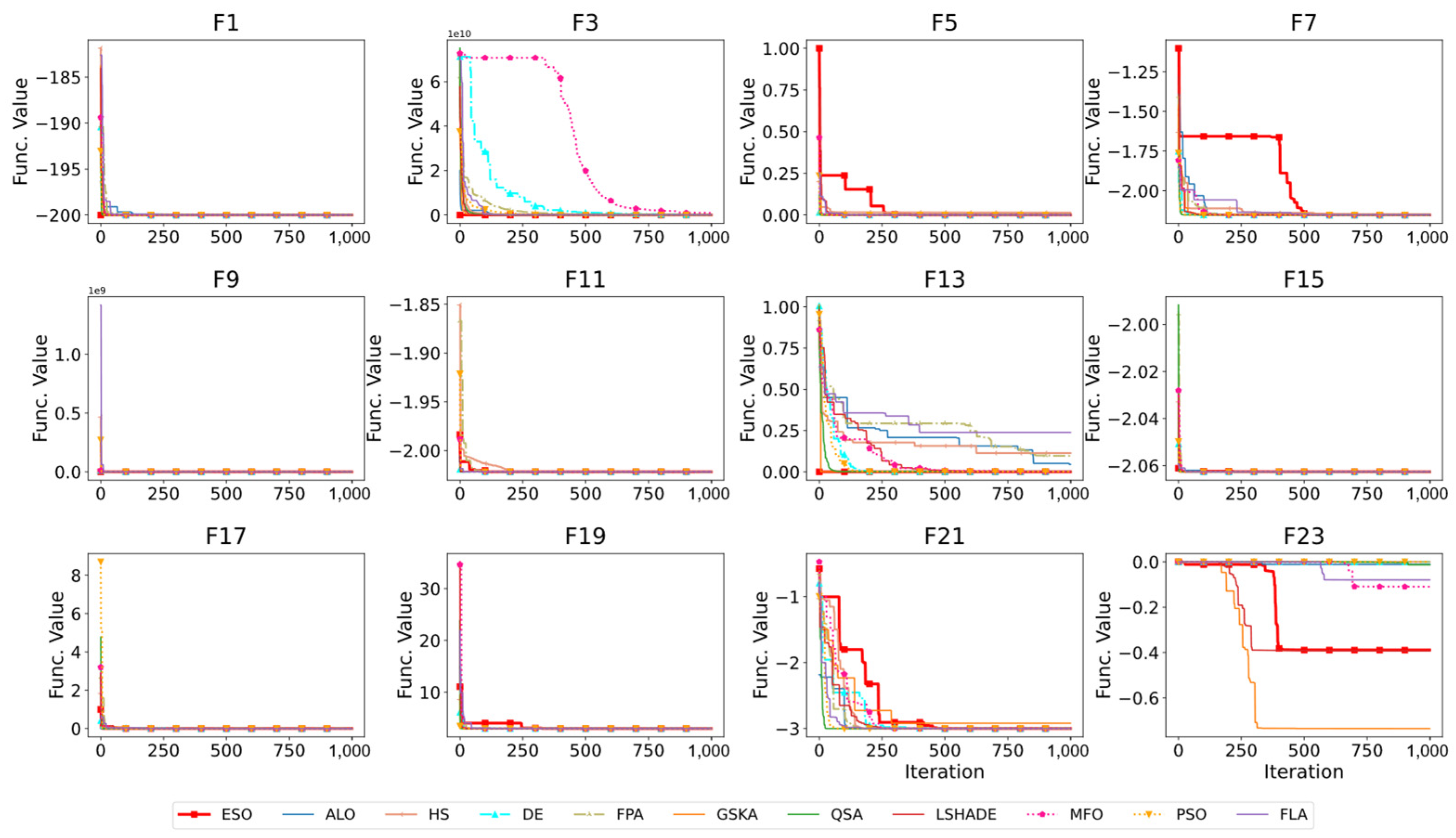
Figure 3 presents the convergence curves of the algorithms across primitive problems. The ESO algorithm demonstrates effective convergence in most of the problems and maintains the lowest function fitness, highlighting its efficiency in exploring and exploiting the solution space. GSKA, LSHADE, and QSA also show strong performance. However, MFO and DE exhibit significant performance variability across different functions.

Benchmark functions in their basic form can lead to misleading performance assessments, particularly due to center bias, which is a common issue where algorithms tend to concentrate their search near the coordinate origin.

Table 4. The rotated, shifted, and rotated benchmark problems, including their bounds, dimensionality (N), optimal solution fitness ($f_{\min \left(x\right)}$), and characteristics, are selected. Linear (L); nonlinear (NL); convex (C); nonconvex (NC); scalable (SC); nonscalable (NSC). The python implementation of the transformed functions can be found in [67].

	Problem Name	Transformation	Bounds	N	Characteristics	${\mathit{f}}_{\mathit{m}\mathit{i}\mathit{n}}\left(\mathit{x}\right)$
F26	Ackley 01	Shifted, Rotated	$-32.7\le x_i\le 32.7$	30	NL, NC, SC	0
F27	Alpine 01	Shifted, Rotated	$-10\le x_i\le 10$	30	NL, NC, SC	0
F28	Booth	Shifted, Rotated	$-10\le x_i\le 10$	2	NL, C, NSC	0
F29	Brown	Shifted, Rotated	$-1\le x_i\le 4$	30	NL, NC, SC	0
F30	Csendes	Shifted, Rotated	$-2\le x_i\le 2$	30	NL, NC, SC	0
F31	Chung Reynolds	Shifted, Rotated	$-100\le x_i\le 100$	30	NL, C, SC	0
F32	Dixon Price	Shifted, Rotated	$-10\le x_i\le 10$	30	NL, C, SC	0
F33	Gulf	Shifted, Rotated	$0\le x_i\le 100$	3	NL, NC, NSC	0
F34	Griewank	Shifted, Rotated	$-600\le x_i\le 600$	30	NL, NC, SC	0
F35	Powell Sum	Shifted, Rotated	$-5\le x_i\le 5$	30	NL, C, SC	0
F36	Penalized 02	Shifted, Rotated	$-50\le x_i\le 50$	30	NL, NC, SC	0
F37	Quartic with Noise	Shifted, Rotated	$-1.28\le x_i\le 1.28$	30	NL, C, SC	0
F38	Ripple 01	Shifted, Rotated	$0\le x_i\le 1$	2	NL, NC, NSC	−2.2
F39	Schwefel 2.21	Shifted, Rotated	$-100\le x_i\le 100$	30	NL, C, SC	0
F40	Sphere	Shifted, Rotated	$-100\le x_i\le 100$	30	NL, C, SC	0
F41	Step 01	Shifted, Rotated	$-100\le x_i\le 100$	30	NL, NC, SC	0
F42	Salomon	Shifted, Rotated	$-100\le x_i\le 100$	30	NL, NC, SC	0
F43	Schaffer 02	Shifted, Rotated	$-100\le x_i\le 100$	30	NL, NC, SC	0
F44	Xin She Yang 02	Shifted, Rotated	$-{\displaystyle \frac{\mathsf{\pi }}{2}}\le x_i\le {\displaystyle \frac{\mathsf{\pi }}{2}}$	30	NL, NC, SC	0
F45	Zakharov	Shifted, Rotated	$-10\le x_i\le 10$	30	NL, C, SC	0

presents transformed benchmark functions, incorporating rotations and shifts to address this limitation. These transformations move optima away from the center and introduce variable interdependencies through orthogonal matrix operations, creating more challenging and realistic test scenarios that better reflect real-world optimization problems. Several studies have shown that algorithms that perform well on basic functions often struggle with these transformed variants, revealing hidden weaknesses in their search mechanisms and potential center bias issues that could impact their practical applications.

The results in

Table 5. Comparison of performance metrics across algorithms for shifted and rotated optimization problems.

Function	Statistics	ESO	ALO	DE	FPA	FLA	GSKA	HS	LSHADE	MFO	PSO	QSA
F26	Mean	6.8 × 10−11	2.5 × 100	1.6 × 100	7.6 × 100	3.5 × 100	8.0 × 10−1	2.2 × 100	7.1 × 10−15	1.0 × 100	1.0 × 101	8.0 × 10−2
	std	4.7 × 10−11	4.0 × 100	5.4 × 10−1	4.5 × 10−1	2.1 × 10−1	6.7 × 10−1	6.8 × 10−1	0.0 × 100	1.1 × 100	3.1 × 100	4.5 × 10−2
	Dist.	6.8 × 10−11	2.5 × 100	1.6 × 100	7.6 × 100	3.5 × 100	8.0 × 10−1	2.2 × 100	7.1 × 10−15	1.0 × 100	1.0 × 101	8.0 × 10−2
F27	Mean	1.1 × 10−1	2.7 × 100	1.8 × 101	1.2 × 101	1.3 × 101	2.2 × 10−2	9.0 × 10−1	7.8 × 10−3	9.7 × 100	6.1 × 100	1.1 × 101
	std	9.4 × 10−2	2.7 × 100	3.1 × 100	9.1 × 10−1	5.1 × 100	1.5 × 10−2	4.9 × 10−1	1.0 × 10−2	4.4 × 100	2.5 × 100	4.2 × 100
	Dist.	1.1 × 10−1	2.7 × 100	1.8 × 101	1.2 × 101	1.3 × 101	2.2 × 10−2	9.0 × 10−1	7.8 × 10−3	9.7 × 100	6.1 × 100	1.1 × 101
F28	Mean	1.5 × 10−9	5.9 × 10−5	2.5 × 100	8.3 × 10−1	3.8 × 100	2.9 × 10−10	1.4 × 100	2.0 × 10−15	5.5 × 101	1.1 × 101	2.9 × 101
	std	2.5 × 10−9	3.7 × 10−5	6.9 × 10−1	10.0 × 10−2	9.1 × 10−1	7.8 × 10−10	3.5 × 10−1	4.4 × 10−15	1.1 × 102	1.3 × 101	6.2 × 101
	Dist.	1.5 × 10−9	5.9 × 10−5	2.5 × 100	8.3 × 10−1	3.8 × 100	2.9 × 10−10	1.4 × 100	2.0 × 10−15	5.5 × 101	1.1 × 101	2.9 × 101
F29	Mean	5.6 × 10−21	5.0 × 10−11	1.6 × 10−3	2.4 × 10−2	7.4 × 10−2	1.6 × 10−21	8.6 × 10−5	3.6 × 10−33	1.2 × 10−1	8.2 × 10−3	1.9 × 100
	std	1.4 × 10−20	1.2 × 10−11	5.9 × 10−4	4.2 × 10−3	3.2 × 10−2	4.7 × 10−21	1.4 × 10−4	4.3 × 10−33	3.5 × 10−1	1.3 × 10−2	2.1 × 100
	Dist.	5.6 × 10−21	5.0 × 10−11	1.6 × 10−3	2.4 × 10−2	7.4 × 10−2	1.6 × 10−21	8.6 × 10−5	3.6 × 10−33	1.2 × 10−1	8.2 × 10−3	1.9 × 100
F30	Mean	2.1 × 10−49	1.7 × 10−10	2.8 × 10−8	2.9 × 10−7	4.4 × 10−7	3.2 × 10−65	3.7 × 10−7	1.4 × 10−75	6.6 × 10−16	9.0 × 10−7	7.7 × 10−13
	std	3.9 × 10−49	4.4 × 10−10	1.9 × 10−8	1.3 × 10−7	2.4 × 10−7	9.7 × 10−65	5.3 × 10−7	4.0 × 10−75	2.0 × 10−15	9.1 × 10−7	8.9 × 10−13
	Dist.	2.1 × 10−49	1.7 × 10−10	2.8 × 10−8	2.9 × 10−7	4.4 × 10−7	3.2 × 10−65	3.7 × 10−7	1.4 × 10−75	6.6 × 10−16	9.0 × 10−7	7.7 × 10−13
F31	Mean	1.7 × 10−45	8.9 × 10−13	1.2 × 101	5.9 × 100	1.1 × 103	5.1 × 10−42	5.5 × 10−2	0.0 × 100	2.2 × 10−27	7.2 × 100	2.3 × 10−5
	std	2.6 × 10−45	1.9 × 10−12	1.6 × 101	2.7 × 100	4.2 × 102	1.5 × 10−41	4.1 × 10−2	0.0 × 100	3.8 × 10−27	1.2 × 101	2.2 × 10−5
	Dist.	1.7 × 10−45	8.9 × 10−13	1.2 × 101	5.9 × 100	1.1 × 103	5.1 × 10−42	5.5 × 10−2	0.0 × 100	2.2 × 10−27	7.2 × 100	2.3 × 10−5
F32	Mean	6.9 × 10−1	1.6 × 100	6.0 × 100	3.4 × 100	1.8 × 101	6.7 × 10−1	5.4 × 100	6.7 × 10−1	7.1 × 10−1	8.2 × 100	8.3 × 10−1
	std	3.5 × 10−2	1.6 × 100	3.2 × 100	5.2 × 10−1	8.9 × 100	2.2 × 10−6	8.8 × 100	1.3 × 10−14	9.1 × 10−2	8.6 × 100	2.4 × 10−1
	Dist.	6.9 × 10−1	1.6 × 100	6.0 × 100	3.4 × 100	1.8 × 101	6.7 × 10−1	5.4 × 100	6.7 × 10−1	7.1 × 10−1	8.2 × 100	8.3 × 10−1
F33	Mean	1.7 × 10−3	2.1 × 10−3	2.2 × 10−3	2.3 × 10−5	1.3 × 10−2	8.9 × 10−3	5.8 × 10−3	6.4 × 10−5	4.8 × 10−3	2.6 × 10−3	1.4 × 10−5
	std	1.1 × 10−3	2.5 × 10−3	1.3 × 10−3	1.7 × 10−5	2.2 × 10−2	6.8 × 10−3	3.3 × 10−3	1.9 × 10−4	2.9 × 10−3	3.9 × 10−3	3.4 × 10−5
	Dist.	1.7 × 10−3	2.1 × 10−3	2.2 × 10−3	2.3 × 10−5	1.3 × 10−2	8.9 × 10−3	5.8 × 10−3	6.4 × 10−5	4.8 × 10−3	2.6 × 10−3	1.4 × 10−5
F34	Mean	4.9 × 10−4	9.3 × 10−4	2.2 × 101	5.1 × 10−2	2.2 × 10−3	6.9 × 10−4	4.4 × 10−3	3.6 × 10−6	1.1 × 101	8.8 × 100	5.3 × 100
	std	4.3 × 10−4	3.2 × 10−4	3.8 × 101	4.7 × 10−2	1.4 × 10−3	2.9 × 10−4	2.8 × 10−3	5.2 × 10−6	2.4 × 101	2.5 × 101	1.6 × 101
	Dist.	4.9 × 10−4	9.3 × 10−4	2.2 × 101	5.1 × 10−2	2.2 × 10−3	6.9 × 10−4	4.4 × 10−3	3.6 × 10−6	1.1 × 101	8.8 × 100	5.3 × 100
F35	Mean	1.1 × 10−21	2.6 × 10−7	1.6 × 100	2.4 × 101	2.2 × 100	4.4 × 10−23	1.6 × 10−2	1.3 × 10−30	1.1 × 10−12	3.4 × 101	4.5 × 10−3
	std	2.1 × 10−21	2.3 × 10−7	1.4 × 100	3.4 × 100	4.4 × 10−1	1.2 × 10−22	2.9 × 10−2	1.2 × 10−30	1.4 × 10−12	1.7 × 101	3.8 × 10−3
	Dist.	1.1 × 10−21	2.6 × 10−7	1.6 × 100	2.4 × 101	2.2 × 100	4.4 × 10−23	1.6 × 10−2	1.3 × 10−30	1.1 × 10−12	3.4 × 101	4.5 × 10−3
F36	Mean	5.4 × 10−2	9.2 × 10−2	6.7 × 10−2	2.5 × 10−1	2.4 × 10−2	6.7 × 10−3	2.2 × 10−2	5.0 × 10−3	2.2 × 10−2	1.5 × 10−1	3.3 × 10−2
	std	6.6 × 10−2	3.1 × 10−2	2.1 × 10−2	1.9 × 10−2	8.6 × 10−3	2.1 × 10−3	7.2 × 10−3	1.5 × 10−3	1.1 × 10−2	9.9 × 10−2	9.3 × 10−3
	Dist.	5.4 × 10−2	9.2 × 10−2	6.7 × 10−2	2.5 × 10−1	2.4 × 10−2	6.7 × 10−3	2.2 × 10−2	5.0 × 10−3	2.2 × 10−2	1.5 × 10−1	3.3 × 10−2
F37	Mean	−2.2 × 100	−2.2 × 100	−2.2 × 100	−1.7 × 100	−2.1 × 100	−2.2 × 100	−1.5 × 100	−2.0 × 100	−2.2 × 100	−1.3 × 100	−2.2 × 100
	std	9.0 × 10−4	1.5 × 10−11	8.4 × 10−4	4.7 × 10−1	1.1 × 10−1	2.4 × 10−3	4.6 × 10−1	3.9 × 10−1	7.9 × 10−4	2.9 × 10−1	4.2 × 10−4
	Dist.	2.2 × 100	2.2 × 100	2.2 × 100	1.7 × 100	2.1 × 100	2.2 × 100	1.5 × 100	2.0 × 100	2.2 × 100	1.3 × 100	2.2 × 100
F38	Mean	8.1 × 10−2	2.0 × 101	6.9 × 100	2.3 × 101	3.7 × 100	1.0 × 10−6	3.4 × 100	2.2 × 10−3	1.3 × 101	1.5 × 101	5.0 × 100
	std	1.1 × 10−1	3.6 × 100	1.1 × 100	3.0 × 100	6.4 × 10−1	7.1 × 10−7	1.6 × 100	2.2 × 10−3	1.1 × 101	7.2 × 100	3.1 × 100
	Dist.	2.3 × 100	2.2 × 101	9.1 × 100	2.5 × 101	5.9 × 100	2.2 × 100	5.6 × 100	2.2 × 100	1.5 × 101	1.7 × 101	7.2 × 100
F39	Mean	1.2 × 10−17	3.7 × 10−7	2.9 × 100	2.2 × 100	2.8 × 101	1.8 × 10−21	1.7 × 10−1	0.0 × 100	3.0 × 10−14	4.3 × 100	5.5 × 10−3
	std	7.6 × 10−18	2.7 × 10−7	1.6 × 100	5.7 × 10−1	7.8 × 100	5.2 × 10−21	4.3 × 10−2	0.0 × 100	6.0 × 10−14	8.0 × 100	3.1 × 10−3
	Dist.	1.2 × 10−17	3.7 × 10−7	2.9 × 100	2.2 × 100	2.8 × 101	1.8 × 10−21	1.7 × 10−1	0.0 × 100	3.0 × 10−14	4.3 × 100	5.5 × 10−3
F40	Mean	0.0 × 100	1.1 × 101	6.5 × 100	4.4 × 101	5.0 × 101	0.0 × 100	1.3 × 100	0.0 × 100	3.5 × 100	1.8 × 102	0.0 × 100
	std	0.0 × 100	2.1 × 100	2.4 × 100	8.5 × 100	1.2 × 101	0.0 × 100	1.1 × 100	0.0 × 100	2.3 × 100	2.2 × 102	0.0 × 100
	Dist.	0.0 × 100	1.1 × 101	6.5 × 100	4.4 × 101	5.0 × 101	0.0 × 100	1.3 × 100	0.0 × 100	3.5 × 100	1.8 × 102	0.0 × 100
F41	Mean	3.6 × 10−1	6.0 × 10−1	1.6 × 100	4.5 × 100	1.2 × 100	2.0 × 10−1	5.6 × 10−1	2.6 × 10−1	6.9 × 10−1	1.8 × 100	8.3 × 10−1
	std	9.2 × 10−2	1.0 × 10−1	3.1 × 10−1	2.0 × 10−1	1.1 × 10−1	1.5 × 10−8	1.2 × 10−1	4.7 × 10−2	1.4 × 10−1	9.3 × 10−1	1.1 × 10−1
	Dist.	3.6 × 10−1	6.0 × 10−1	1.6 × 100	4.5 × 100	1.2 × 100	2.0 × 10−1	5.6 × 10−1	2.6 × 10−1	6.9 × 10−1	1.8 × 100	8.3 × 10−1
F42	Mean	1.8 × 10−16	3.7 × 10−2	4.6 × 10−1	4.9 × 10−1	1.0 × 10−1	5.3 × 10−16	2.4 × 10−2	2.2 × 10−16	6.3 × 10−4	4.9 × 10−2	2.6 × 10−1
	std	8.9 × 10−17	6.6 × 10−2	1.0 × 10−2	1.5 × 10−3	1.8 × 10−2	1.1 × 10−16	2.3 × 10−2	0.0 × 100	1.5 × 10−3	6.9 × 10−2	5.8 × 10−2
	Dist.	1.8 × 10−16	3.7 × 10−2	4.6 × 10−1	4.9 × 10−1	1.0 × 10−1	5.3 × 10−16	2.4 × 10−2	2.2 × 10−16	6.3 × 10−4	4.9 × 10−2	2.6 × 10−1
F43	Mean	2.6 × 10−11	2.5 × 10−7	2.9 × 10−6	1.1 × 10−9	7.7 × 10−9	1.2 × 10−6	1.1 × 10−6	1.9 × 10−10	1.5 × 10−6	8.3 × 10−8	3.9 × 10−7
	std	1.9 × 10−11	7.6 × 10−7	1.6 × 10−6	4.4 × 10−10	1.2 × 10−8	6.3 × 10−7	8.6 × 10−7	1.1 × 10−10	2.3 × 10−6	1.1 × 10−7	5.0 × 10−7
	Dist.	2.6 × 10−11	2.5 × 10−7	2.9 × 10−6	1.1 × 10−9	7.7 × 10−9	1.2 × 10−6	1.1 × 10−6	1.9 × 10−10	1.5 × 10−6	8.3 × 10−8	3.9 × 10−7
F44	Mean	2.9 × 10−6	8.5 × 10−1	2.2 × 102	8.6 × 101	3.1 × 100	6.3 × 101	6.2 × 101	2.6 × 10−2	4.7 × 101	6.5 × 101	1.5 × 101
	std	7.5 × 10−6	9.1 × 10−1	2.4 × 101	1.2 × 101	6.8 × 10−1	1.7 × 101	1.7 × 101	3.9 × 10−2	2.1 × 101	4.0 × 101	4.1 × 100
	Dist.	2.9 × 10−6	8.5 × 10−1	2.2 × 102	8.6 × 101	3.1 × 100	6.3 × 101	6.2 × 101	2.6 × 10−2	4.7 × 101	6.5 × 101	1.5 × 101
F45	Mean	0.0 × 100	1.0 × 100	3.2 × 100	1.1 × 100	2.0 × 100	3.1 × 100	3.0 × 100	2.2 × 10−1	2.1 × 100	1.5 × 100	1.0 × 100
	std	0.0 × 100	4.8 × 10−3	8.4 × 10−1	3.2 × 10−2	3.4 × 10−1	9.9 × 10−1	1.4 × 100	4.5 × 10−1	9.2 × 10−1	4.7 × 10−1	5.6 × 10−2
	Dist.	0.0 × 100	1.0 × 100	3.2 × 100	1.1 × 100	2.0 × 100	3.1 × 100	3.0 × 100	2.2 × 10−1	2.1 × 100	1.5 × 100	1.0 × 100

reveal differential performance patterns across the shifted and rotated functions (F26–F45). ESO and LSHADE maintain their optimization capabilities, with ESOs achieving exceptional precision in functions such as F26, F35, F31, F39, and F40. However, several algorithms exhibit significant performance degradation when confronted with these transformed variants. The FLA and PSO struggled considerably, as evidenced by substantial deviations in F31 (1.1 × 10³) and F40 (1.8 × 10²), respectively. DE and ALO showed intermediate performance, but lacked consistency, particularly in challenging cases such as F44, where DE reached 2.2 × 10². GSKA emerged as a notably resilient algorithm, maintaining strong performance across several transformed functions, especially F30 and F39 (distances of 3.2 × 10⁻⁶⁵ and 1.8 × 10⁻²¹). These results underscore the significant impact of rotational and shift transformations on optimization algorithm performance, highlighting the importance of developing algorithms with invariance to such transformations. This pattern suggests that the introduction of rotation and shift transformations substantially increases the complexity of the optimization landscape, challenging algorithms that rely heavily on coordinate-wise optimization strategies or which might be indicators of design biases, as reported previously [18].

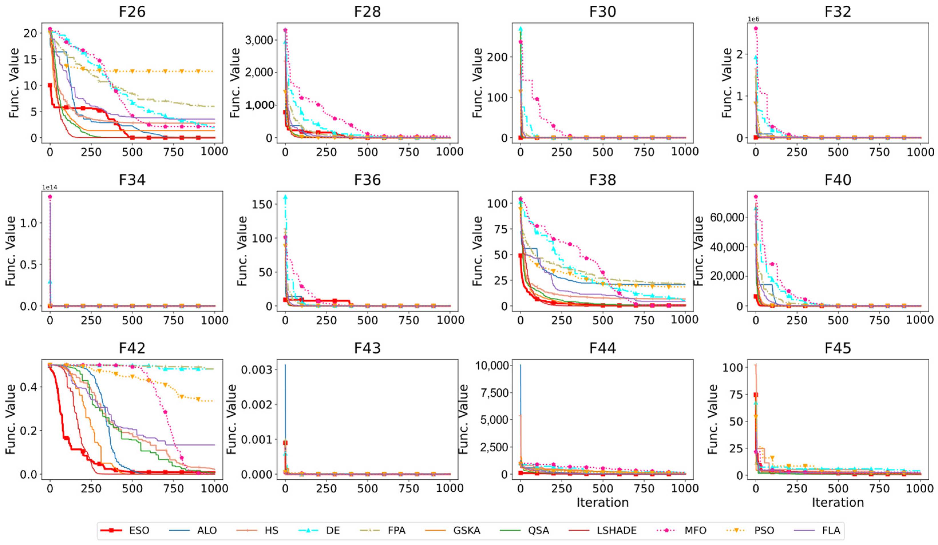
Similarly, Figure 4 shows the convergence curves of the algorithms for shifted and rotated problems. ESO and LSHADE consistently demonstrated rapid convergence to the lowest function fitness, indicating efficiency in finding optimal solutions. Conversely, the algorithms DE, MFO, and PSO displayed significant performance variability across different functions, showing generally slower or poorer convergence.

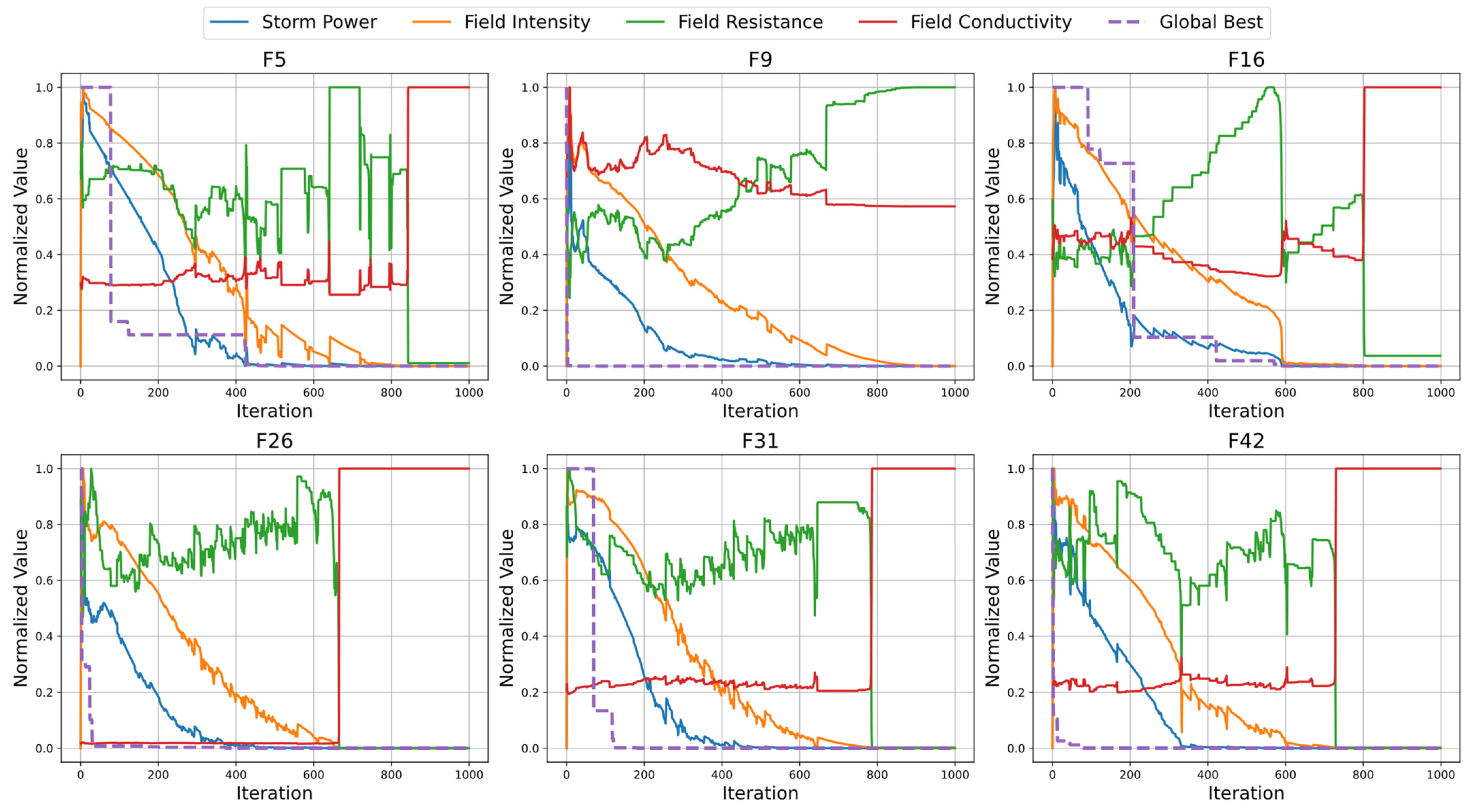
Internal Parameter Behavior

Analysis across benchmark functions (F5, F9, F16, F26, F31, and F42) reveals distinct trends in the behaviors of the three main internal parameters of the ESO algorithm, field resistance ($R$), field conductivity ($ke$), and field intensity ($I$), as shown in Figure 5. The behavior of $R$ changes with the evolution of the problem’s landscape, describing the diversity of solutions at each iteration. Conversely, $ke$ is complementary and reactive to $R$, controlling the transition from exploration to exploitation. As $R$ decreases, $ke$ adjusts to favor exploitation, focusing on the promising regions of the search space. The field intensity generally follows a decreasing pattern over iterations, but can also increase when sudden changes in $R$ and $ke$ occur. This keeps the search agents responsive to the landscape, allowing for both steady convergence and rapid adjustment to new promising areas. The progression in the global best solution is a direct result of the interplay between $R$, $ke$, and $I$. This adaptability enables the ESO algorithm to effectively navigate complex search spaces, achieving consistent improvements toward the global optimum.

3.2. CEC 2022 SOBC Benchmark Problems

The CEC SOBC 2022 suite, detailed in

Table 6. CEC 2022 Bound constrained single objective optimization problem characteristics.

Function	Type	Problem	${\mathit{f}}_{\mathit{m}\mathit{i}\mathit{n}}\left(\mathit{x}\right)$
F46	Shifted–rotated primitive functions	Shifted and fully rotated Zakharov	300
F47		Shifted and fully rotated Rosenbrock	400
F48		Shifted and fully rotated expanded Schaffer 06	600
F49		Shifted and fully rotated Non-Continuous Rastringin	800
F50		Shifted and fully rotated Levy	900
F51	Hybrid functions	Hybrid Function 1 (N = 3)	1800
F52		Hybrid Function 2 (N = 6)	2000
F53		Hybrid Function 3 (N = 5)	2200
F54	Composition function	Composition Function 1 (N = 5)	2300
F55		Composition Function 2 (N = 4)	2400
F56		Composition Function 3 (N = 5)	2600
F57		Composition Function 4 (N = 6)	2700
Bounds: $-100\le x_i\le 100$; Dimension = [10, 20]

, is designed to rigorously test optimization algorithms in demanding scenarios using transformations such as rotations and shifts in the optimum [27]. These elements are critical for examining an algorithm’s robustness and adaptability in nonlinear high-dimensional search spaces. Additionally, the suite features hybrid and composite functions that amalgamate various problem types into a single test, increasing computational demands and complexity. This thorough evaluation not only tests the algorithm’s ability to manage intricate optimization tasks, but also provides deep insights into its applicability and limitations under challenging conditions.

In

Table 7. Comparison of performance metrics across algorithms for the CEC SOBC 2022 problems for D = 10.

Function	Statistics	ESO	ALO	DE	FPA	FLA	GSKA	HS	LSHADE	MFO	PSO	QSA
D = 10
F46	Mean	3.0 × 102	3.0 × 102	3.0 × 102	3.0 × 102	3.0 × 102	3.0 × 102	3.0 × 102	3.0 × 102	3.0 × 102	3.0 × 102	3.0 × 102
	std	0.0 × 100	1.6 × 10−9	0.0 × 100	2.7 × 10−4	1.1 × 100	2.3 × 10−14	4.8 × 10−4	0.0 × 100	6.0 × 10−14	5.7 × 10−14	7.2 × 10−11
	Dist.	0.0 × 100	3.4 × 10−9	0.0 × 100	8.4 × 10−4	1.7 × 100	0.0 × 100	7.0 × 10−4	0.0 × 100	0.0 × 100	5.7 × 10−14	3.9 × 10−11
F47	Mean	4.0 × 102	4.1 × 102	4.1 × 102	4.0 × 102	4.1 × 102	4.1 × 102	4.1 × 102	4.1 × 102	4.1 × 102	4.1 × 102	4.1 × 102
	std	8.1 × 10−2	1.4 × 101	2.4 × 100	9.0 × 10−3	1.9 × 100	4.1 × 100	1.0 × 101	2.9 × 100	1.5 × 100	2.2 × 101	1.0 × 101
	Dist.	2.1 × 10−1	9.5 × 100	6.7 × 100	8.3 × 10−3	7.9 × 100	5.7 × 100	7.1 × 100	7.0 × 100	7.5 × 100	1.3 × 101	8.1 × 100
F48	Mean	6.0 × 102	6.0 × 102	6.0 × 102	6.0 × 102	6.0 × 102	6.0 × 102	6.0 × 102	6.0 × 102	6.0 × 102	6.0 × 102	6.0 × 102
	std	0.0 × 100	7.9 × 10−14	0.0 × 100	6.1 × 10−10	9.7 × 10−6	2.3 × 10−14	8.7 × 10−9	0.0 × 100	6.0 × 10−14	1.0 × 10−13	0.0 × 100
	Dist.	0.0 × 100	1.1 × 10−13	0.0 × 100	1.3 × 10−9	1.9 × 10−5	0.0 × 100	1.3 × 10−8	0.0 × 100	0.0 × 100	0.0 × 100	0.0 × 100
F49	Mean	8.3 × 102	8.5 × 102	8.5 × 102	8.3 × 102	8.3 × 102	8.3 × 102	8.2 × 102	8.1 × 102	8.4 × 102	8.5 × 102	8.3 × 102
	std	1.1 × 101	2.4 × 101	8.6 × 100	7.1 × 100	1.5 × 101	6.9 × 100	7.5 × 100	2.9 × 100	1.3 × 101	1.7 × 101	9.0 × 100
	Dist.	3.3 × 101	4.9 × 101	4.6 × 101	3.2 × 101	3.4 × 101	3.1 × 101	2.2 × 101	1.3 × 101	3.6 × 101	4.8 × 101	3.0 × 101
F50	Mean	9.0 × 102	9.0 × 102	9.0 × 102	9.0 × 102	9.0 × 102	9.0 × 102	9.0 × 102	9.0 × 102	9.0 × 102	9.0 × 102	9.0 × 102
	std	3.2 × 10−1	3.0 × 10−1	0.0 × 100	8.8 × 10−2	2.0 × 10−3	7.5 × 10−14	6.3 × 10−2	0.0 × 100	1.4 × 10−13	6.7 × 10−1	1.6 × 10−1
	Dist.	1.5 × 10−1	3.3 × 10−1	0.0 × 100	6.9 × 10−2	3.0 × 10−3	0.0 × 100	6.8 × 10−2	0.0 × 100	0.0 × 100	6.8 × 10−1	7.2 × 10−2
F51	Mean	2.7 × 104	3.1 × 104	1.8 × 103	1.8 × 103	3.5 × 104	4.7 × 104	1.4 × 104	1.8 × 103	4.0 × 104	8.2 × 103	1.3 × 104
	std	1.2 × 104	2.0 × 104	3.7 × 10−1	9.5 × 100	1.4 × 104	1.8 × 104	7.6 × 103	2.9 × 10−1	6.9 × 103	5.0 × 103	1.8 × 104
	Dist.	2.5 × 104	2.9 × 104	7.0 × 10−1	3.3 × 101	3.4 × 104	4.5 × 104	1.2 × 104	4.3 × 10−1	3.8 × 104	6.4 × 103	1.1 × 104
F52	Mean	2.0 × 103	2.0 × 103	2.0 × 103	2.0 × 103	2.0 × 103	2.0 × 103	2.0 × 103	2.0 × 103	2.0 × 103	2.0 × 103	2.0 × 103
	std	8.7 × 100	1.4 × 101	9.1 × 100	3.0 × 100	7.5 × 100	2.5 × 100	8.8 × 100	5.7 × 100	1.3 × 101	8.3 × 100	9.2 × 100
	Dist.	2.7 × 101	3.4 × 101	2.5 × 101	3.3 × 101	2.3 × 101	3.4 × 101	1.5 × 101	4.6 × 100	3.7 × 101	2.9 × 101	2.8 × 101
F53	Mean	2.2 × 103	2.3 × 103	2.2 × 103	2.2 × 103	2.2 × 103	2.2 × 103	2.2 × 103	2.2 × 103	2.2 × 103	2.2 × 103	2.3 × 103
	std	6.5 × 100	1.9 × 102	4.7 × 100	3.7 × 100	4.5 × 100	4.7 × 100	4.6 × 101	6.3 × 100	7.8 × 100	4.6 × 100	5.1 × 102
	Dist.	2.6 × 101	1.0 × 102	1.7 × 101	1.9 × 101	2.3 × 101	2.7 × 101	4.8 × 101	6.6 × 100	2.0 × 101	2.2 × 101	1.3 × 102
F54	Mean	2.3 × 103	2.6 × 103	2.6 × 103	2.3 × 103	2.6 × 103	2.5 × 103	2.6 × 103	2.4 × 103	2.7 × 103	2.4 × 103	2.7 × 103
	std	0.0 × 100	1.7 × 102	1.5 × 102	2.8 × 10−2	1.4 × 102	1.7 × 102	1.6 × 102	1.4 × 102	1.9 × 10−2	1.5 × 102	9.0 × 101
	Dist.	0.0 × 100	2.7 × 102	2.7 × 102	9.7 × 10−2	2.9 × 102	1.5 × 102	2.7 × 102	7.2 × 101	3.6 × 102	8.5 × 101	3.6 × 102
F55	Mean	2.6 × 103	1.7 × 103	8.2 × 102	8.6 × 102	3.2 × 102	1.6 × 103	1.6 × 103	9.1 × 102	3.0 × 102	1.3 × 103	6.8 × 102
	std	1.6 × 102	1.0 × 103	6.7 × 102	1.9 × 102	6.7 × 102	6.9 × 102	7.8 × 102	5.9 × 102	8.1 × 102	9.9 × 102	8.9 × 102
	Dist.	1.5 × 102	7.1 × 102	1.6 × 103	1.5 × 103	2.1 × 103	8.2 × 102	8.5 × 102	1.5 × 103	2.1 × 103	1.1 × 103	1.7 × 103
F56	Mean	2.6 × 103	2.7 × 103	2.6 × 103	2.5 × 103	2.6 × 103	2.6 × 103	2.6 × 103	2.6 × 103	2.7 × 103	2.6 × 103	2.6 × 103
	std	2.6 × 10−13	2.4 × 102	2.3 × 10−10	3.1 × 102	1.2 × 10−1	1.7 × 102	1.7 × 102	0.0 × 100	2.8 × 102	7.5 × 100	1.4 × 101
	Dist.	0.0 × 100	8.2 × 101	4.7 × 10−10	6.3 × 101	3.5 × 10−1	3.4 × 101	4.0 × 101	0.0 × 100	1.1 × 102	2.7 × 100	9.9 × 100
F57	Mean	2.9 × 103	2.9 × 103	2.8 × 103	2.7 × 103	2.8 × 103	2.8 × 103	2.5 × 103	2.8 × 103	2.8 × 103	2.8 × 103	2.8 × 103
	std	1.7 × 101	5.5 × 100	1.6 × 101	1.5 × 102	6.6 × 101	1.4 × 101	3.2 × 102	1.7 × 101	1.2 × 102	2.1 × 102	6.0 × 101
	Dist.	1.8 × 102	1.6 × 102	1.4 × 102	1.6 × 101	10.0 × 101	1.4 × 102	1.7 × 102	1.4 × 102	1.0 × 102	8.7 × 101	1.3 × 102
D = 20
F46	Mean	3.0 × 102	3.0 × 102	3.0 × 102	3.1 × 102	3.2 × 102	3.0 × 102	3.0 × 102	3.0 × 102	3.5 × 102	3.0 × 102	3.0 × 102
	std	5.7 × 10−14	6.9 × 10−9	3.6 × 10−1	2.6 × 100	6.9 × 100	0.0 × 100	4.7 × 10−2	0.0 × 100	1.6 × 102	2.2 × 10−5	5.5 × 10−2
	Dist.	5.7 × 10−14	2.4 × 10−8	4.4 × 10−1	9.6 × 100	2.4 × 101	1.1 × 10−13	5.2 × 10−2	0.0 × 100	4.7 × 101	4.9 × 10−6	2.0 × 10−2
F47	Mean	4.4 × 102	4.6 × 102	4.5 × 102	4.5 × 102	4.6 × 102	4.7 × 102	4.5 × 102	4.4 × 102	4.5 × 102	4.5 × 102	4.5 × 102
	std	2.0 × 101	1.9 × 101	2.1 × 100	1.1 × 101	2.1 × 101	8.6 × 100	9.0 × 100	1.6 × 101	2.0 × 100	2.3 × 101	1.6 × 101
	Dist.	4.0 × 101	6.1 × 101	4.7 × 101	4.7 × 101	6.0 × 101	6.6 × 101	5.4 × 101	4.3 × 101	4.8 × 101	4.7 × 101	4.6 × 101
F48	Mean	6.0 × 102	6.0 × 102	6.0 × 102	6.0 × 102	6.0 × 102	6.0 × 102	6.0 × 102	6.0 × 102	6.0 × 102	6.0 × 102	6.0 × 102
	std	6.4 × 10−14	2.5 × 10−13	2.5 × 10−8	1.6 × 10−6	1.5 × 10−4	2.3 × 10−14	1.4 × 10−7	0.0 × 100	5.6 × 10−14	2.4 × 10−7	8.6 × 10−11
	Dist.	0.0 × 100	1.0 × 10−12	4.3 × 10−8	6.7 × 10−6	3.3 × 10−4	1.1 × 10−13	3.1 × 10−7	0.0 × 100	1.1 × 10−13	4.9 × 10−8	1.3 × 10−10
F49	Mean	9.0 × 102	9.6 × 102	1.0 × 103	9.3 × 102	9.4 × 102	9.7 × 102	9.6 × 102	8.5 × 102	9.4 × 102	9.7 × 102	9.4 × 102
	std	3.1 × 101	5.5 × 101	2.5 × 101	1.9 × 101	3.5 × 101	2.3 × 101	1.9 × 101	9.8 × 100	4.7 × 101	4.9 × 101	3.9 × 101
	Dist.	1.0 × 102	1.6 × 102	2.3 × 102	1.3 × 102	1.4 × 102	1.7 × 102	1.6 × 102	4.6 × 101	1.4 × 102	1.7 × 102	1.4 × 102
F50	Mean	9.0 × 102	9.0 × 102	9.0 × 102	9.0 × 102	9.0 × 102	9.0 × 102	9.0 × 102	9.0 × 102	9.0 × 102	9.0 × 102	9.0 × 102
	std	7.7 × 10−1	1.3 × 100	5.8 × 10−4	6.6 × 10−1	2.3 × 100	2.7 × 10−1	9.2 × 10−2	1.8 × 10−2	8.5 × 10−1	2.2 × 100	1.1 × 100
	Dist.	9.5 × 10−1	2.7 × 100	4.2 × 10−4	1.8 × 100	2.4 × 100	2.2 × 10−1	1.1 × 10−1	3.6 × 10−3	5.2 × 10−1	4.2 × 100	1.3 × 100
F51	Mean	6.9 × 104	5.8 × 104	6.9 × 105	5.6 × 104	3.6 × 105	2.7 × 107	4.4 × 104	1.5 × 104	1.4 × 105	5.8 × 104	1.2 × 106
	std	1.9 × 104	1.9 × 104	5.1 × 105	1.3 × 104	1.7 × 105	1.4 × 107	1.4 × 104	5.8 × 103	3.9 × 104	2.2 × 104	5.7 × 106
	Dist.	6.7 × 104	5.6 × 104	6.8 × 105	5.4 × 104	3.6 × 105	2.7 × 107	4.2 × 104	1.3 × 104	1.4 × 105	5.6 × 104	1.2 × 106
F52	Mean	2.0 × 103	2.1 × 103	1.9 × 103	2.0 × 103	2.0 × 103	2.0 × 103	2.0 × 103	1.9 × 103	1.9 × 103	2.0 × 103	2.0 × 103
	std	7.9 × 101	2.2 × 102	3.0 × 101	3.1 × 101	1.3 × 102	9.1 × 101	7.8 × 101	7.9 × 101	5.5 × 101	8.5 × 101	8.3 × 101
	Dist.	1.8 × 101	1.0 × 102	6.0 × 101	3.9 × 101	5.4 × 100	7.6 × 100	3.5 × 101	7.0 × 101	1.2 × 102	1.6 × 101	2.5 × 101
F53	Mean	2.5 × 103	2.7 × 103	2.1 × 103	2.1 × 103	2.8 × 103	1.9 × 104	2.9 × 103	2.2 × 103	4.0 × 103	2.7 × 103	2.5 × 103
	std	2.3 × 102	3.8 × 102	2.0 × 102	2.6 × 101	4.3 × 102	2.0 × 104	6.7 × 102	7.4 × 101	1.5 × 103	6.9 × 102	6.1 × 102
	Dist.	3.3 × 102	5.3 × 102	6.5 × 101	1.0 × 102	5.7 × 102	1.6 × 104	7.2 × 102	2.2 × 101	1.8 × 103	5.3 × 102	2.9 × 102
F54	Mean	2.3 × 103	2.6 × 103	2.6 × 103	2.6 × 103	2.6 × 103	2.6 × 103	2.6 × 103	2.6 × 103	2.6 × 103	2.7 × 103	2.7 × 103
	std	0.0 × 100	6.9 × 101	6.4 × 10−3	1.0 × 102	4.4 × 100	3.2 × 10−5	2.5 × 100	4.5 × 10−13	2.5 × 100	2.9 × 101	5.4 × 101
	Dist.	0.0 × 100	3.4 × 102	3.4 × 102	2.8 × 102	3.4 × 102	3.4 × 102	3.4 × 102	3.4 × 102	3.4 × 102	3.8 × 102	3.6 × 102
F55	Mean	2.2 × 103	1.0 × 103	2.6 × 103	4.7 × 102	1.2 × 102	2.7 × 103	8.6 × 102	5.0 × 102	5.3 × 102	7.2 × 102	1.5 × 103
	std	9.1 × 102	1.2 × 103	4.1 × 102	3.3 × 102	9.6 × 102	2.4 × 102	1.4 × 103	1.7 × 103	1.1 × 103	1.6 × 103	1.1 × 103
	Dist.	2.1 × 102	1.4 × 103	2.1 × 102	1.9 × 103	2.3 × 103	2.6 × 102	1.5 × 103	1.9 × 103	1.9 × 103	1.7 × 103	8.9 × 102
F56	Mean	2.6 × 103	2.8 × 103	2.6 × 103	2.6 × 103	2.6 × 103	2.6 × 103	2.6 × 103	2.6 × 103	2.6 × 103	2.6 × 103	3.1 × 103
	std	4.5 × 10−13	4.4 × 102	1.1 × 10−2	8.8 × 10−2	5.4 × 100	4.5 × 10−13	1.2 × 101	0.0 × 100	1.4 × 101	1.4 × 101	6.9 × 102
	Dist.	4.5 × 10−13	1.8 × 102	2.3 × 10−2	4.8 × 10−1	3.2 × 100	1.4 × 10−12	9.1 × 100	0.0 × 100	1.8 × 101	1.1 × 101	4.9 × 102
F57	Mean	3.0 × 103	3.0 × 103	2.9 × 103	3.0 × 103	2.9 × 103	2.9 × 103	2.9 × 103	2.9 × 103	2.9 × 103	3.0 × 103	3.0 × 103
	std	4.3 × 101	3.2 × 101	9.2 × 100	2.9 × 101	1.5 × 101	1.2 × 101	1.2 × 101	8.1 × 100	8.7 × 100	8.5 × 101	2.2 × 101
	Dist.	3.1 × 102	2.8 × 102	2.3 × 102	2.7 × 102	2.4 × 102	2.3 × 102	2.3 × 102	2.2 × 102	2.3 × 102	3.1 × 102	2.6 × 102

, the results for optimizing the CEC SOBC 2022 competition problems reveal distinct performance patterns across different dimensionalities. For D = 10, ESO and LSHADE demonstrated superior performance, with ESOs achieving optimal or near-optimal results in several functions, particularly F46, F48, F54, and F56 (distances of 0.0 × 10⁰).

For D = 20, while most algorithms experienced performance degradation, ESO and LSHADE maintained relative stability. ESO particularly excelled in F46, F48, and F56 (distance of 0.0 × 10⁰), although it showed increased sensitivity in F51, where the distance rose from 2.5 × 10⁴ at D=10 to 6.7 × 10⁴ at D = 20. LSHADE demonstrated robust scalability, maintaining consistent performance across dimensions, notably for F46, F48, and F56 (distances of 0.0 × 10⁰).

The remaining algorithms showed significant performance deterioration with increased dimensionality. This was particularly evident in the results of GSKA for F51, where the distance increased dramatically from 4.5 × 10⁴ at D = 10 to 2.7 × 10⁷ at D = 20. Similar degradation patterns were observed in FLA and PSO, indicating their limited ability to handle higher-dimensional search spaces effectively. Notably, specific functions such as F49 and F55 proved to be challenging across all algorithms and dimensions, suggesting inherent complexity in these problem landscapes that warrant further investigation for algorithm improvement.

3.3. Real-World Bound Constrained Optimization Problems

While artificial benchmark functions are commonly employed to assess the performance and accuracy of metaheuristic algorithms, such synthetic problems often embed unrealistic properties that may not be representative of real-world scenarios. As a result, evaluations can lead to overestimations or underestimations of the true potential of an algorithm when it is applied outside of controlled test conditions. To address this gap and provide a more precise assessment, we submit the ESO algorithm and its comparative metaheuristics to the challenge of solving four diverse and complex problems from real-world engineering and industrial domains.

3.3.1. Lennard–Jones Potential Problem

The Lennard–Jones potential problem is a fundamental challenge in molecular physics, which focuses on determining the optimal spatial configuration of atoms that minimizes the total potential energy of the system. For a 15-molecule system, this represents a 45-dimensional optimization problem (3 spatial coordinates per molecule), with a theoretical minimum potential that corresponds to the most stable molecular configuration.

The objective function sums the pairwise interaction potentials between all molecules as $V\left(r\right)=4\epsilon \left[{\left({\displaystyle \frac{\sigma }{r}}\right)}^{12}-{\left({\displaystyle \frac{\sigma }{r}}\right)}^6\right]$, where $r$ is the distance between molecules, $\epsilon$ is the depth of the potential well, and $\sigma$ is the distance at which the potential becomes zero. The optimization aims to minimize the total potential energy $VN\left(p\right)=\Sigma \Sigma \left(r_{ij}^{-12}-2r_{ij}^{-6}\right)$, which is subjected to geometric constraints. The complete implementation of the problem can be found in [68]. The problem’s complexity stems from its highly multimodal nature, featuring numerous local minima corresponding to different stable configurations. The global minimum represents the most energetically favorable molecular arrangement, making this a valuable benchmark for testing the ability of optimization algorithms to navigate complex energy landscapes. The complete implementation of the problem can be found in [69].

In

Table 8. Performance comparison of different algorithms on the Lennard–Jones potential problem. The values show position coordinates (ranging from −2 to +2) for 15 particles and the final objective function value (Cost).

	ESO	ALO	DE	FPA	FLA	GSKA	HS	LSHADE	MFO	PSO	QSA
$x_1$	1.434865	1.359019	−1.970468	−0.014599	0.365808	−0.470226	0.586455	1.208653	−1.138859	−1.009291	1.712633
$x_2$	1.191828	0.336952	−1.490921	−0.736735	−1.005121	0.803350	−0.394619	−0.783929	−1.999048	−1.275606	1.182789
$x_3$	0.699767	0.577357	1.142062	0.199979	−0.965342	−0.307276	−0.421156	0.659644	1.624503	0.222959	1.504628
$x_4$	1.999970	0.896645	−1.167551	−0.398293	1.244353	0.352321	−0.155720	0.242997	−0.436711	−0.501022	2.000000
$x_5$	1.115344	−0.140981	−2.000000	0.015786	−1.388556	0.548935	0.259772	−1.044061	−1.475131	−0.715828	2.000000
$x_6$	1.518684	−0.140981	1.456385	−0.331072	−1.235420	−0.863945	−0.550639	0.764147	1.146678	0.879632	1.002105
$x_7$	1.175422	0.606547	−2.000000	0.437363	0.532327	−0.183326	−0.208390	−0.334759	−1.984282	−0.121675	1.230942
$x_8$	1.683618	0.817785	−2.000000	0.156283	−1.227329	−0.196021	−0.640118	−0.302973	−1.973537	−0.893590	1.455159
$x_9$	1.528411	−0.106009	2.000000	0.196516	−1.914800	−0.256384	−0.978713	0.436202	1.094949	−0.026080	0.674214
$x_{10}$	2.000000	−0.140981	−2.000000	−0.247618	−0.362616	0.317509	−0.301950	0.532111	−1.105097	−1.492482	2.000000
$x_{11}$	1.989568	−0.140981	−0.989352	0.872546	−1.420013	−0.399401	−0.549758	−0.504754	−2.000000	−0.627814	2.000000
$x_{12}$	1.999880	−0.140981	2.000000	0.179714	−1.517291	−1.055094	0.014254	−0.017795	0.623619	0.808372	2.000000
$x_{13}$	1.976906	−0.140981	−2.000000	−0.448235	0.430119	0.716317	0.206446	0.524449	−1.387533	−0.910924	1.133734
$x_{14}$	1.973133	−0.140981	−2.000000	0.029733	−1.960166	0.721455	−1.316111	−0.095083	−1.173953	−0.290672	1.999975
$x_{15}$	1.002376	−0.140981	2.000000	0.660970	−1.248826	0.033407	−0.373104	0.895740	1.114318	0.070847	1.504609
Cost	−9.103852	−5.837872	−8.219488	−9.091091	−9.094731	−6.671860	−9.103852	−9.098313	−9.103852	−9.103852	−9.103852

, the results for the Lennard–Jones potential optimization problem with 15 particles reveal distinct performance patterns among the tested algorithms. ESO, HS, MFO, PSO, and the QSA achieve perfect convergence, reaching the exact known optimal value of −9.103852. This consistent achievement across multiple algorithms validates the robustness of these methods for this molecular configuration problem.

FPA, FLA, and LSHADE demonstrated near-optimal performance, achieving values of −9.091091, −9.094731, and −9.098313, respectively, with deviations of less than 0.15% from the global optimum. However, other algorithms struggled significantly, with ALO showing the poorest performance (−5.837872) followed by GSKA (−6.671860) and DE (−8.219488), suggesting that these methods may require modifications to better handle this specific type of molecular optimization problem.

3.3.2. Tersoff Potential Problem—Si(B) Model

The Tersoff Potential Problem for silicon, specifically the Si(B) parameterization, focuses on determining the minimum energy configuration of silicon atoms in a molecular cluster. This problem models covalent bonding interactions with a sophisticated three-body potential function that accounts for bond order and angular dependencies.

The optimization objective represents the total potential energy $f\left(X_1,\dots ,X_3\right)=E_1\left(X_1,\dots ,X_3\right)+\dots +E\left(X_1,\dots ,X_3\right)$, where each atomic contribution $E_{\mathrm{i}}$ includes the following:

• Two-body repulsive and attractive terms.
• Bond-order term incorporating angular effects.
• Cutoff function for limiting the interaction range.

The total potential is the sum of the individual potentials of atoms $E_i={\displaystyle \frac{1}{2}}\sum _{j\ne i}{f}_c\left(r_{ij}\right)\left(V_R\left(r_{ij}\right)-B_{ij}{V}_R\left(r_{ij}\right)\right)$, where $r_{ij}$ is the distance between atoms $i$ and $j$, $V_R$ is a repulsive term, $f_c\left(r_{ij}\right)$ is a switching function, and $B_{ij}$ is a many-body term that depends on the position of the atoms $i$ and $j$. The complete implementation of the problem can be found in [69].

In

Table 9. Performance comparison for the Tersoff Potential Problem—Si(B) Model. The values show the atomic position coordinates (bounded between −2 and +2) for 30 particles and the final objective function value (Cost).

	ESO	ALO	DE	FPA	FLA	GSKA	HS	LSHADE	MFO	PSO	QSA
$x_1$	1.911343	−0.422796	1.944408	0.286240	1.416869	−0.274498	1.875122	2.000000	0.094775	−0.372801	−0.252995
$x_2$	1.837886	0.216275	0.367359	0.287359	0.253849	2.000000	−0.029182	−0.080788	1.827431	−0.001320	1.062548
$x_3$	1.830802	−2.000000	−0.456927	1.682189	2.000000	0.727327	−1.737446	−2.000000	0.372470	−1.999627	−1.999950
$x_4$	−1.576741	−1.380137	0.516711	0.423848	0.442175	0.003527	−1.756877	−0.375639	0.912800	−0.052452	−1.231063
$x_5$	−0.132260	0.001101	−0.229355	−1.485867	−0.488212	2.000000	−0.179581	−0.102737	−1.500830	2.000000	0.273089
$x_6$	1.020404	1.130858	0.800000	0.059508	−0.073051	−2.000000	1.811431	−2.000000	0.272097	−0.029351	0.980519
$x_7$	0.665033	1.491677	−1.421290	−0.635832	−1.739788	1.044658	1.917820	0.114731	2.000000	−1.277256	0.773974
$x_8$	−0.169312	1.670233	0.764938	1.824677	0.484076	−2.000000	−1.774767	−1.847730	0.474414	1.450233	−1.999004
$x_9$	2.000000	−2.000000	1.871599	0.309387	−0.093171	−0.996529	−0.028274	−0.308888	−0.402388	1.826011	1.903878
$x_{10}$	0.613636	1.776506	−2.000000	−1.662366	−1.031304	2.000000	1.839513	0.971574	−2.000000	−0.605600	1.238730
$x_{11}$	2.000000	1.016080	−0.134894	0.201058	1.977085	1.751415	−0.064260	−1.652146	0.818365	−1.815764	0.014669
$x_{12}$	−0.823520	1.970005	−0.800000	−1.429618	1.561238	−0.658564	1.675033	2.000000	1.158593	−0.545546	0.791099
$x_{13}$	−0.140903	1.938587	−2.000000	1.561017	−0.882716	−2.000000	−0.126871	0.672269	0.590976	−1.945784	0.233157
$x_{14}$	−1.997927	−0.706526	2.000000	−0.605732	−0.300260	0.360569	1.555238	2.000000	1.366157	−0.458269	2.000000
$x_{15}$	0.672988	0.358969	−1.412000	−1.815761	1.941022	0.484315	1.840499	0.733992	−1.999789	0.718484	0.083112
$x_{16}$	−0.173769	−1.262689	0.250558	−1.880201	2.000000	−0.543066	−1.695519	1.632626	−1.408305	−2.000000	−2.000000
$x_{17}$	−0.333620	−1.572003	−0.160011	−1.658721	−1.872017	−0.320085	−0.229380	−0.160240	−1.209102	1.269511	−0.325520
$x_{18}$	−1.095456	−0.655218	−2.000000	0.096784	1.145205	−1.203856	−1.714797	0.453970	0.221774	−0.904993	−1.252132
$x_{19}$	−0.417366	0.895856	−0.655298	−0.726259	1.020043	−2.000000	−0.094898	−0.246328	0.916364	1.995465	1.999995
$x_{20}$	1.999937	−1.640321	−2.000000	−1.707307	2.000000	−2.000000	−0.365644	0.308474	−0.919850	1.114406	−1.999782
$x_{21}$	1.373192	−1.519072	2.000000	−1.956821	0.542941	2.000000	0.074306	2.000000	−1.999914	−0.015754	−0.148793
$x_{22}$	−1.657211	0.424965	0.087166	1.722122	−0.004664	2.000000	−1.809800	−1.661183	−1.332842	0.830348	−0.377947
$x_{23}$	1.532557	1.106551	2.000000	1.282008	1.482053	2.000000	1.395652	−0.365374	−0.067126	−1.279863	−1.739322
$x_{24}$	−0.647209	0.004665	2.000000	0.200628	−1.401937	2.000000	0.092705	0.235537	−1.809520	1.183456	−0.201882
$x_{25}$	2.000000	0.100960	2.000000	−1.982998	2.000000	−1.166635	1.487776	0.980895	−0.050179	1.558506	1.012128
$x_{26}$	0.289188	−1.810179	−1.512233	0.204361	−1.969780	−2.000000	1.489119	2.000000	−0.067582	−0.927549	−0.949578
$x_{27}$	0.026378	1.227828	−2.000000	1.452503	−1.145471	0.042998	0.059791	−1.854988	1.931138	−0.998212	−2.000000
$x_{28}$	1.668289	−0.361096	−0.427233	0.473964	1.870840	−2.000000	0.235857	−1.054432	−1.999995	0.924628	−1.993408
$x_{29}$	−1.901752	1.979633	−1.700175	1.455288	0.215631	2.000000	−1.763749	1.750140	1.998915	0.847429	1.908550
$x_{30}$	−0.784580	2.000000	−0.422944	−1.822801	−1.927111	−1.535681	−1.841567	−0.732077	−0.856910	1.999620	−0.585655
Cost	−42.175192	−40.514917	−30.258289	−42.888543	−41.701543	−32.093009	−40.802206	−42.698791	−44.074326	−43.129095	−42.192469

, the results for the Tersoff potential Si(B) model optimization reveal that MFO achieves the best performance, with a minimum value of −44.074326, followed closely by PSO (−43.129095) and the FPA (−42.888543). LSHADE, ESO, and QSA also showed competitive performance, reaching values of −42.698791 and −42.192469, respectively, demonstrating strong capabilities in handling this complex molecular potential optimization. However, FLA and HS produced slightly higher values of −41.701543 and −40.802206, respectively. However, some algorithms struggled significantly with this problem, particularly DE and GSKA, which only reached values of −30.258289 and −32.093009, respectively, indicating substantial difficulty in navigating this specific potential energy landscape. Significant performance differences were found, with nearly 14 energy units between the best and worst results.

3.3.3. Spread Spectrum Radar Polyphase Code Design Problem

The Spread Spectrum Radar Polyphase Code Design Problem represents a critical optimization challenge in radar signal processing. The fundamental objective is to design optimal polyphase codes that enable effective radar pulse compression while minimizing undesirable side lobes in the compressed signal output. The problem is structured as a global minimization task of a maximum function. The objective function seeks to minimize the maximum side-lobe level across all possible phase combinations as $f\left(x\right)=\mathrm{m}\mathrm{a}\mathrm{x}({\phi }_1\left(x\right),\dots ,{\phi }_m(x\left)\right)$, where ${\phi }_i\left(x\right)=0.5+\sum _{j=1^n}\mathrm{c}\mathrm{o}\mathrm{s}\left(\sum _{k=2i-j+i^k}{x}_k\right)$. Here, $x$ represents the vector of phase variables $(x_1,x_2,\dots ,x_n)$, $k$ is the phase accumulation index, and ${\phi }_i$ is the normalized autocorrelation. The optimization space consists of 20 phase variables, each constrained within the interval [0, 2π]. This creates a continuous search space with complex periodic behaviors. The objective function exhibits multiple local minima, making it particularly challenging for optimization algorithms to locate the global optimum. The complete implementation of the problem can be found in [69].

In

Table 10. Optimization results for the Spread Spectrum Radar Polyphase Code Design Problem. The values show phase angles (bounded between −π and π radians) for a 30-element code sequence and the final objective function value (Cost).

	ESO	ALO	DE	FPA	FLA	GSKA	HS	LSHADE	MFO	PSO	QSA
$x_1$	−3.100815	−1.520351	−0.965774	0.544349	−3.036591	3.141593	−1.518217	2.557269	−1.345045	3.112985	−3.141593
$x_2$	0.332067	−2.121173	0.637765	1.360767	−3.041196	−1.932973	2.954669	0.671064	0.334946	−2.546519	−2.760456
$x_3$	−2.574641	−1.105060	−3.141593	2.333700	1.201947	−3.141593	−2.664397	−2.753454	0.942050	−0.316298	−2.923732
$x_4$	−0.545815	−1.319132	−1.432463	1.964902	2.012501	3.141593	−2.423320	−2.291713	3.132594	−1.697346	−0.288332
$x_5$	1.141980	1.665574	1.851032	2.377952	0.072295	−1.106539	−1.237725	−2.419544	−2.445811	−1.277584	1.268597
$x_6$	1.120970	−1.762508	−3.141593	−2.236733	0.204019	2.149439	−1.862466	3.141593	−0.967030	−2.688296	−0.333390
$x_7$	1.282702	−0.653277	1.246695	−0.342986	−3.141593	1.607691	−2.845321	2.979361	1.669502	1.401700	−0.084430
$x_8$	−2.321864	−3.139784	0.860463	2.044107	2.254097	0.685412	−1.893046	−1.116027	2.811512	−0.283606	−3.141593
$x_9$	−0.183235	−3.107299	3.141593	1.221318	−1.062995	−1.809399	−1.246318	−0.356383	−1.212574	0.126748	0.299340
$x_{10}$	2.491207	−2.991052	−3.141593	−0.072572	−0.387584	−2.191098	−1.361084	0.456348	0.751910	−0.365913	−1.517103
$x_{11}$	−3.066385	−0.290439	1.752981	−1.263895	0.887252	2.958228	−0.014845	0.173017	1.037721	2.976465	−1.732491
$x_{12}$	−1.942425	−1.862323	−3.141593	2.917213	2.652048	−3.141593	−2.002796	−1.309828	−0.124584	−0.898133	2.381386
$x_{13}$	−0.710979	−1.120679	−3.141593	2.243351	−2.446711	−2.013341	2.791427	−2.526366	−2.461666	1.220693	2.236986
$x_{14}$	−2.541145	0.477636	0.026919	2.164634	1.835622	−2.413783	−1.128471	−0.417597	−0.149518	1.184910	−1.610186
$x_{15}$	−1.767841	−1.530916	−1.391671	2.723396	−0.090144	−0.066451	−2.489393	0.711040	2.971660	2.559379	−2.850798
$x_{16}$	−1.499577	−0.237383	0.148266	1.770362	−3.004787	−1.423347	−0.926059	1.126406	1.931100	−1.806416	−3.141593
$x_{17}$	2.902179	0.670926	3.141593	−2.887093	−2.917292	1.758365	−0.616175	1.283235	−1.421458	−0.026777	0.185552
$x_{18}$	−2.249648	−2.129232	−3.141593	−1.281230	−2.006409	3.141593	−0.995523	2.264549	−0.473386	−2.703633	−3.141593
$x_{19}$	−2.897327	−3.120522	0.948639	3.045817	2.781638	0.743333	−0.512369	2.941368	−2.866881	−2.300161	−3.141593
$x_{20}$	2.369769	−3.080855	3.141593	−0.563177	1.723770	−3.141593	2.826144	−2.623419	−1.295967	1.011977	−3.038621
$x_{21}$	−1.680448	−3.131099	0.036346	0.163516	0.194469	3.141593	0.349376	0.186491	1.764819	−2.003619	−1.858572
$x_{22}$	2.949012	−3.138728	0.855628	−0.409861	−1.376177	−0.370307	0.422910	−2.990428	1.048934	2.780416	−0.333768
$x_{23}$	3.106054	−1.667111	3.141593	−2.546677	−0.550574	0.248312	−1.610595	−0.084111	−0.558064	1.409432	−2.219474
$x_{24}$	−1.043635	−0.199998	1.507456	2.452170	2.278041	−2.564327	1.207318	−2.160056	−2.243206	−1.218152	−2.642824
$x_{25}$	1.896537	−3.132711	−3.141593	−1.742223	−1.661561	0.481999	1.645104	−0.438920	2.066923	−0.299825	−3.019206
$x_{26}$	−0.634534	−0.068603	2.048128	0.769361	−3.141593	−1.216155	−0.600581	3.140928	−0.074927	0.222078	−3.141593
$x_{27}$	2.399096	−2.768813	2.278858	−2.627048	−1.005585	−3.141593	0.357423	−1.637072	1.600227	−1.520878	0.504020
$x_{28}$	−0.094720	−2.861763	3.141593	1.685769	−3.095756	−1.279020	0.397469	−0.403978	−1.002799	−1.686028	1.779107
$x_{29}$	−0.975141	−2.000241	−3.141593	−2.672582	0.441302	−1.405712	2.816245	−0.729825	−2.085518	−1.118786	0.142481
$x_{30}$	−1.407476	−2.189864	3.069431	1.838584	−0.707854	−0.985931	−2.426521	2.111333	0.913540	0.898270	−3.134029
Cost	1.980246	2.448449	3.398476	2.623724	2.609190	3.562859	3.279291	2.433395	2.762012	2.680859	2.943761

, the results for the Spread Spectrum Radar Polyphase Code Design Problem demonstrate that the ESO achieves the best performance, with a minimum cost value of 1.980246, followed closely by LSHADE (2.433395) and ALO (2.448449). These results indicate superior capabilities in optimizing the phase sequences for radar signal design.

The FLA and FPA showed similar performance levels, reaching cost values of 2.609190 and 2.623724, respectively, demonstrating moderate effectiveness in this specialized optimization task. However, the GSKA encountered significant challenges, producing the highest cost value of 3.562859, followed by DE with 3.398476 and HS with 3.279291, suggesting that these algorithms struggle with the specific constraints and complexity of radar code design.

3.3.4. Circular Antenna Array Optimization Problem

The circular antenna array optimization problem addresses the design of antenna arrays arranged in a circular configuration to achieve optimal radiation patterns. This problem has significant applications in radar systems, mobile communications, and satellite technology. The array factor ($AF$) for a circular antenna array with $N$ elements is expressed as $AF\left(\phi \right)=\sum _{n=i^N}{I}_{\mathrm{n}}\exp \left[j_{kr}\left(\cos \left(\phi -{\phi }_n\right)-\cos \left({\phi }_0-{\phi }_n\right)\right)+{\beta }_n\right]$, where $\phi$ represents the azimuth angle in the x–y plane, $I_{\mathrm{n}}$ denotes the amplitude excitation of the n-th element, $k$ is the wavenumber, $r$ defines the radius of the circle, ${\phi }_0$ indicates the direction of maximum radiation, ${\beta }_n$ is the phase excitation of the n-th element, and $N$ is the total number of array elements. The optimization aims to minimize a composite objective $f=\left|{\displaystyle \frac{AR\left({\phi }_{\mathrm{sll}},I,\beta \right)}{AR\left({\phi }_{\max },I,\beta \right)}}\right|+{\displaystyle \frac{1}{DIR\left({\phi }_0,I,\beta \right)}}+\left|{\phi }_1-\phi d_{\mathrm{es}}\right|+\sum _{k=1^k}\left|AR\left({\phi }_{\mathrm{k}},I,\beta \right)\right|$, where ${\phi }_{\mathrm{sll}}$ represents the angle at which the maximum side lode occurs, $DIR$ denotes the directivity of the array pattern, $\phi d_{\mathrm{es}}$ is the desired maximum radiation direction, and ${\phi }_{\mathrm{k}}$ specifies the k-th null control direction. The optimization is constrained to current amplitudes ($I_n$) [0.2, 1.0] and phase excitation (${\beta }_n$) [$-180°, 180°$]. The complete implementation of the problem can be found in [69].

In

Table 11. Performance comparison of different algorithms in the circular antenna array optimization problem. The values show the current excitation amplitudes ($x_1-x_8$) (bounded between 0.2 and 1.0) and phase angles ($x_9-x_{16}$) (bounded between 0° and 360°) for an eight-element array.

	ESO	ALO	DE	FPA	FLA	GSKA	HS	LSHADE	MFO	PSO	QSA
$x_1$	0.826762	0.655702	0.372293	0.500000	0.453294	0.562055	0.665949	0.993508	0.300000	0.500000	0.655702
$x_2$	0.580678	122.373515	88.521081	196.971756	148.888920	48.534188	91.641661	111.606724	134.172623	196.971756	122.373515
$x_3$	0.787151	0.550832	0.536435	0.500000	0.386820	0.488968	0.650500	0.972003	0.298481	0.500000	0.550832
$x_4$	0.174480	243.992739	168.318334	301.023384	278.675256	65.965652	170.193613	236.185596	247.334374	301.023384	243.992739
$x_5$	0.003385	0.293068	0.252116	0.500421	0.546207	0.058893	0.247977	0.706625	0.412725	0.500421	0.293068
$x_6$	0.205614	258.297786	163.448644	282.596030	277.002108	94.839997	162.211812	228.595121	204.884861	282.596030	258.297786
$x_7$	0.802547	0.423961	0.485756	0.500000	0.533680	0.617781	0.673747	0.917669	0.299854	0.500000	0.423961
$x_8$	0.643657	123.843239	93.118729	206.797952	143.240209	64.137762	84.180194	108.903852	101.663546	206.797952	123.843239
$x_9$	0.012882	0.566155	0.446070	0.598747	0.503816	0.338813	0.089852	0.100289	0.388761	0.598747	0.566155
$x_{10}$	206.062613	251.590723	155.823200	197.431070	179.665472	114.471955	228.478716	249.013508	225.031970	197.431070	251.590723
$x_{11}$	0.991110	0.469193	0.428587	0.774321	0.493968	0.083279	0.899603	0.899999	0.516478	0.774321	0.469193
$x_{12}$	186.934931	282.100443	149.944308	194.385970	240.317196	88.092418	263.197623	278.136398	189.887400	194.385970	282.100443
$x_{13}$	0.496933	0.443013	0.404401	0.590189	0.615920	0.010942	0.774288	0.647830	0.411243	0.590189	0.443013
$x_{14}$	181.735020	42.562513	166.138240	240.690145	119.455936	71.325032	142.867142	124.350970	143.955945	240.690145	42.562513
$x_{15}$	0.007159	0.447668	0.444143	0.708113	0.609304	0.000000	0.387422	0.200441	0.472467	0.708113	0.447668
$x_{16}$	160.088913	120.490818	156.254987	199.814598	213.820034	42.269511	167.539353	124.217988	194.639459	199.814598	120.490818
Cost	−11.479936	−4.361428	−5.199967	−3.974214	−4.366539	−4.743778	−7.211993	−6.009528	−4.336477	−3.974214	−4.361428

, the results for the circular antenna array optimization problem demonstrate that the ESO achieved significantly superior performance, with a cost value of −11.479936, substantially outperforming all the other algorithms. HS emerged as the second-best performer, with a cost of −7.211993, followed by LSHADE at −6.009528.

DE and the GSKA achieved moderate performance levels, with costs of −5.199967 and −4.743778, respectively, whereas the remaining algorithms clustered around similar performance levels between −4.3 and −4.4. The FPA and PSO showed the least effective performance, both reaching a cost of −3.974214, indicating difficulty in optimizing the antenna array parameters.

4. Discussion

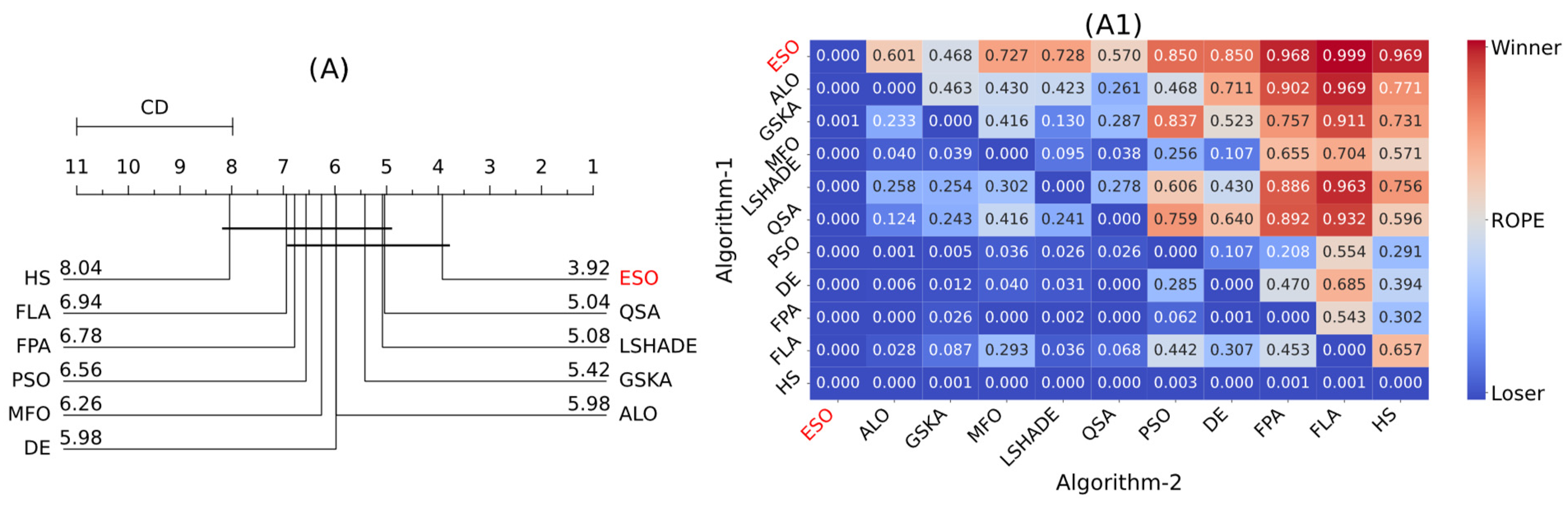
4.1. Statistical Performance Evaluation

Two statistical tests were employed to evaluate the optimization results. A Bayesian signed-rank test was employed to identify differences in mean fitness between populations, providing a more robust and comprehensive analysis than traditional nonparametric tests do [70]. Furthermore, a critical differences (CD) analysis via Friedman’s test with the Nemenyi post hoc test was conducted to compute the individual rankings and the critical differences [71]. The statistical analysis was conducted on 11 populations comprising 40,700 paired samples divided into 3 groups of problems (Figure 6A–C) and the total set of problems (Figure 6D). The familywise significance level for the tests was set to alpha = 0.05. The null hypothesis, which posited that all populations were normally distributed, was rejected (p = 0.000) for every population and set of problems. The median (MD) and median absolute deviation (MAD) were reported for each population. The populations were assessed pairwise to determine whether they were smaller, equal, or larger. A decision was made in favor of one of these outcomes if the estimated posterior probability was at least alpha = 0.05. The effect size was used to define the region of practical equivalence (ROPE), dynamically calculated around the median as $0.100\ast \mathsf{\Gamma }$, where $\mathsf{\Gamma }$ is the effect size (Akinshin’s gamma) [71].

Based on the results presented, the following conclusions can be drawn about the performance of the ESO algorithm compared to that of the other algorithms:

(a)

For the primitive problems (Figure 6A,A1), ESO and LSHADE exhibited the best performances, with minimal differences between them. The pairwise comparison in Figure 6A clearly shows that the ESO has superior performance.

(b)

For the shifted and rotated problems (Figure 6B,B1), the ESO and LSHADE algorithms again achieved the best performances, with a more noticeable difference between their results and those of the other algorithms. Critical differences were found between the performances of the PSO, FLA, DE, and MFO algorithms and those of the other methods. The pairwise comparison in Figure 6B also reveals that the ESO has superior performance.

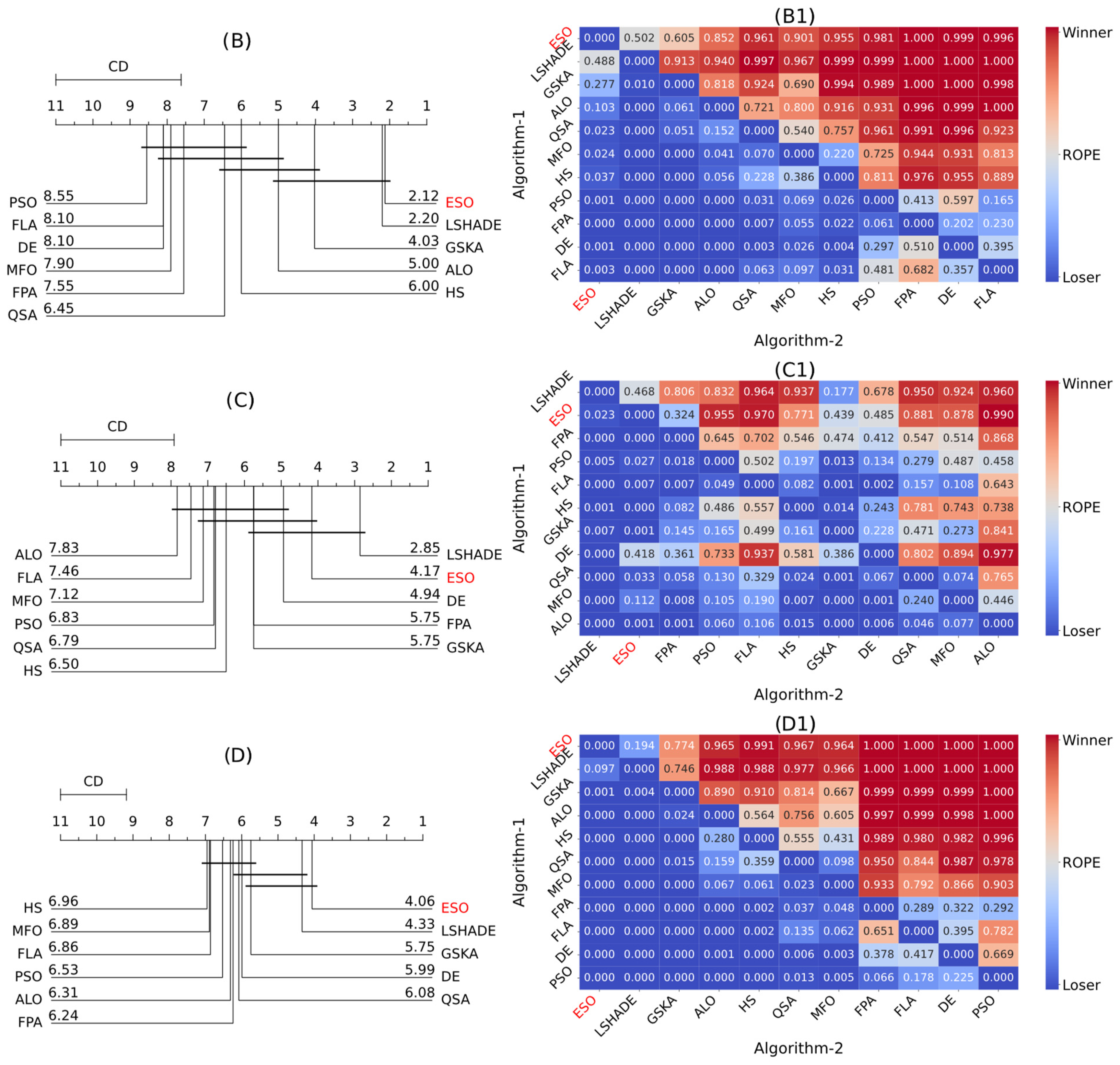
(c)

In the CEC SOBC 2022 problems (Figure 6C,C1), LSHADE leads, followed by ESO. The pairwise comparison revealed that LSHADE had a slightly greater performance.

(d)

Among the three sets of problems, the ESO (4.06) ranks first, followed by LSHADE (4.33) and GSKA (5.75) (Figure 6D,D1).

These outcomes emphasize the ability of the ESO to adapt and excel across a broad range of optimization challenges, demonstrating its potential as a versatile and effective tool for solving complex problems under various conditions.

4.2. Computational Overhead

The computational cost of the ESO algorithm can be analyzed via ‘Big O’ notation, which is a well-established notation in computer sciences, to provide a theoretical estimate of its complexity. This analysis helps in understanding how the algorithm scales with respect to various parameters under typical usage scenarios. The asymptotic complexity of the ESO algorithm is heavily influenced by the number of iterations, the number of repetitions, and the complexity of the objective function. The dimensionality of the problem also plays a significant role, especially in how vector and matrix calculations are handled within the algorithm. Thus, the computational load of the algorithm presented herein can be theoretically estimated as follows:

(a)

Lightning initialization: Initializing each lightning event involves at least one evaluation of the objective function and operations over a vector of size $dim$. The complexity of this part is $O\left(lightnings\times T\left(f\right)\right)$, where $T\left(f\right)$ represents the complexity of evaluating the objective function.

(b)

Main loop:

• Identifying ionized areas: Sorting lightning events based on their fitness has a complexity of $O\left(lightnings\times \log \left(lightnings\right)\right)$.
• Field intensity adjustment and resistance calculation: These calculations have a complexity of $O\left(lightnings\times dim\right)$ since they involve computing the standard deviation and the peak-to-peak difference across the lightning positions.
• Lightning propagation: Each lightning event may adjust its position based on the ionized areas, potentially requiring another evaluation of the objective function, $O\left(lightnings\times T\left(f\right)\right)$.

(c)

Total function evaluations: Each lightning strike evaluates the objective function at least once per iteration, $O\left(maxiter\times lightnings\times T\left(f\right)\right)$.

Combining all these components, the overall computational complexity of the ESO algorithm can be estimated as in Equation (15):

$$\mathit{O}(\mathbf{m}\mathbf{a}\mathbf{x}\_\mathit{i}\mathit{t}\mathit{e}\mathit{r}\times \mathit{l}\mathit{i}\mathit{g}\mathit{h}\mathit{t}\mathit{n}\mathit{i}\mathit{n}\mathit{g}\mathit{s}\times (\mathit{T}\left(\mathit{f}\right)+\mathbf{l}\mathbf{o}\mathbf{g}\left(\mathit{l}\mathit{i}\mathit{g}\mathit{h}\mathit{t}\mathit{n}\mathit{i}\mathit{n}\mathit{g}\mathit{s}\right)+\mathit{d}\mathit{i}\mathit{m}\left)\right)$$

(15)

Additionally, to evaluate the computational complexity of the algorithm in terms of execution time, we applied the CEC SOBC 2022 evaluation procedure [43]. The problem in Equation (16) executes a loop with 200,000 iterations, where, in each step, the value of the variable x is modified through a series of mathematical operations. T0 represents the time calculated by running the test problem in Equation (16). Meanwhile, T1 represents the time required to execute 200,000 independent evaluations of the benchmark function F51 in D dimensions. $\hat{T}$2, on the other hand, refers to the average time taken to execute the same number of evaluations of F51 within the framework of the algorithms in five runs, also in D dimensions. The analysis of the computational complexity across various optimization algorithms shown in

Table 12. Computational complexity analysis of the optimization algorithms using the CEC 2022 SOBC procedure. T0 represents the base time, T1 is the environment time to solve F51, and $\widehat{T}2$ is the mean time of each algorithm to solve F51. (T2 − T1)/T0 calculates the overhead.

Algorithm	$\mathit{T}0$	$\mathit{T}1$		$\widehat{\mathit{T}}2$		$\frac{\widehat{\mathit{T}}2-\mathit{T}1}{\mathit{T}0}$
		D = 10	D = 20	D = 10	D = 20	D = 10	D = 20
ALO	0.0923	0.6551	0.6722	8.27	10.43	82.508227	105.7498929
DE	0.0900			8.06	10.17	82.326846	105.5637776
FPA	0.0910			8.15	10.29	82.406834	105.6458533
FLS	0.0856			7.67	9.68	81.952697	105.1798627
HS	0.0890			7.97	10.06	82.245061	105.4798575
GSKA	0.1756			16.32	22.51	89.207859	124.3610478
LSHADE	0.1320			11.83	14.92	84.642856	107.9402422
MFO	0.1070			9.59	12.09	83.483305	106.7504234
PSO	0.1022			9.16	11.55	83.195754	106.455367
QSA	0.1125			10.08	12.72	83.782624	107.0575553
ESO	0.0350			3.14	3.66	70.885714	85.25142857

reveals significant differences in performance between algorithms and dimensions. In increasing dimensions, all algorithms show heightened execution times, underscoring the added complexity with higher dimensions. Notably, the ESO demonstrates lower overheads, suggesting greater efficiency in handling higher-dimensional tasks. All the experiments were carried out in the following computational environment:

• OS: Ubuntu Linux 24.04 LTS;
• CPU: Intel^® Xeon^® Gold 6148 CPU@2.40 GHz;
• RAM: 64 GB;
• Language: Python 3.12.3.

$$\mathit{x}=\mathbf{0.55};\mathit{x}=\mathit{x}+\mathit{x};\mathit{x}={\displaystyle \frac{\mathit{x}}{\mathbf{2}}};\mathit{x}=\mathit{x}\ast \mathit{x};\mathit{x}=\sqrt{\mathit{x}};\mathit{x}=\mathbf{log}\left(\mathit{x}\right);\mathit{x}=\mathbf{exp}\left(\mathit{x}\right);\mathit{x}={\displaystyle \frac{\mathit{x}}{\mathit{x}+\mathbf{2}}}$$

(16)

4.3. Comparison with Gradient-Based Methods

While gradient-based optimization methods remain fundamental in mathematical programming, particularly for problems with well-defined structures, the ESO algorithm offers distinct characteristics that make it suitable for specific optimization scenarios. A careful examination of both approaches reveals their complementary nature and specific domains of applicability.

Gradient-based methods excel in problems with smooth, differentiable objective functions, offering rapid convergence and mathematical guarantees of optimality when applied to convex optimization problems. These methods are particularly efficient in low- to medium-dimensional problems where gradient information is analytically available. Furthermore, for problems with clear mathematical formulations, such as linear programming or convex quadratic programming, gradient-based methods provide robust theoretical convergence properties.

In contrast, the ESO demonstrates advantages in several challenging scenarios where gradient-based methods may struggle. First, the field resistance mechanism of the ESO enables the effective navigation of multimodal landscapes, allowing for it to escape from local optima through its dynamic exploration–exploitation balance. Second, since the ESO operates solely on function evaluations, it can handle nondifferentiable objectives and discontinuous functions without modification. Third, the algorithm’s field intensity and conductivity parameters provide adaptive search capabilities that maintain optimization momentum in regions where gradient information becomes unreliable or vanishes, such as plateau regions or near-flat landscapes.

This advantage becomes particularly evident in high-dimensional problems where gradient computation through numerical differentiation becomes computationally expensive or impractical. While gradient-based methods need to evaluate the objective function multiple times to approximate each partial derivative, the ESO maintains consistent computational complexity regardless of dimensionality, making it potentially more efficient for high-dimensional optimization tasks.

These considerations suggest that the choice between the ESO and gradient-based methods should be guided by problem characteristics rather than treating either approach as universally superior. The ESO is particularly suited for complex optimization problems with limited mathematical structure, multimodal landscapes, high dimensionality, or where gradient information is unreliable or computationally expensive to obtain. Conversely, gradient-based methods remain the preferred choice for well-structured low-dimensional convex optimization problems where analytical derivatives are available.

5. Conclusions

In this research, the electrical storm optimization (ESO) algorithm is presented as a novel population-based metaheuristic inspired by the dynamic behavior observed in electrical storms. The algorithm operates primarily through three parameters that are dynamically adjusted according to the optimized landscape: field resistance, field conductivity and field intensity. These parameters are crucial because they allow for the algorithm to transition between exploration and exploitation phases effectively. Field resistance is utilized to measure the dispersion of solutions within the search space, providing insights that guide the algorithm’s adjustments based on the problem’s topology. Field conductivity dynamically modulates the algorithm’s adaptability to the optimization landscape, enabling it to respond sensitively to changes in field resistance and facilitating the fine-tuning of the search process. Field intensity controls the phases of the algorithmic process, facilitating strategic shifts between exploration and exploitation.

The performance of the ESO algorithm was thoroughly evaluated across various sets of problems. It was particularly effective in addressing 25 primitive problems characterized by complex landscapes, where it demonstrated high precision and stability. The algorithm also displayed high capabilities in resolving 20 shifted and rotated problems. To test the algorithm further, it was tested against 12 advanced problems from the CEC 2022 suite. Statistical analysis, including the Bayesian signed-rank test and critical difference (CD) analysis via Friedman’s test with the Nemenyi post hoc test, indicated that the performance of the ESO was significantly better than that of several established methods, ranking first overall, closely followed by LSHADE. However, it was observed that the precision of the ESO slightly diminished in the monotonous optimization landscapes, indicating a potential area for further refinement.

In practical applications, the ESO demonstrated effectiveness in solving four complex engineering problems involving molecular processes and antenna design problems, particularly those characterized by nonconvex search spaces and multiple local optima. While classical optimization methods such as gradient-based approaches remain superior for problems with clear mathematical formulations and convex landscapes, the performance of the ESO in these six case studies suggests its utility for specific engineering scenarios where traditional methods may face limitations, such as problems with nondifferentiable objectives or deceptive local optima. These real-world implementations highlight the potential of the ESO as a complementary tool in the optimization toolbox, which is particularly suitable for complex problems where the objective function landscape is not well understood or where classical optimization methods may struggle to find global solutions.

Limitations and Future Works

The current implementation of the ESO presents several limitations that should be acknowledged. The basic constraint-handling mechanism using penalty functions may not be optimal for problems with complex feasibility landscapes. The algorithm’s formulation assumes continuous search spaces, which limits its effectiveness in discrete optimization problems. Experimental validation, while being comprehensive for static optimization, does not include dynamic optimization problems where the optimum changes over time, leaving this capability unexplored. The algorithm’s applicability to multiobjective problems currently relies on aggregating multiple objectives into a single function, which may limit the accuracy of the Pareto front approximation. Additionally, the dynamic parameter adaptation strategy might require more iterations to achieve convergence in extremely deceptive or monotonic landscapes.

Future research directions could address these limitations through several key developments. The advancement of constraint-handling mechanisms based on adaptive penalty functions or feasibility rules would enhance the algorithm’s ability to handle complex constraints. The algorithm could be extended to discrete optimization through appropriate modifications of the field parameters and branching mechanisms, while adaptation for dynamic optimization problems could be achieved by incorporating time-varying field properties. The framework could be reformulated for true multiobjective optimization without requiring objective aggregation. Additionally, enhancing the parameter adaptation mechanism would enable faster convergence in deceptive landscapes. The integration of local search strategies would improve performance in monotonic search spaces, and the development of hybrid versions would combine the ESO’s global exploration capabilities with problem-specific local search methods. These developments significantly expand the algorithm’s applicability while addressing its current limitations.