Article

Enhanced Graph Representation Convolution: Effective Inferring Gene Regulatory Network Using Graph Convolution Network with Self-Attention Graph Pooling Layer

by
Duaa Mohammad Alawad
1,
Ataur Katebi
2,3 and
Md Tamjidul Hoque
1,*
1
Computer Science, University of New Orleans, 2000 Lakeshore Drive, Math 308, New Orleans, LA 70148, USA
2
Department of Bioengineering, Northeastern University, Boston, MA 02115, USA
3
Center for Theoretical Biological Physics, Northeastern University, Boston, MA 02115, USA
*
Author to whom correspondence should be addressed.
Mach. Learn. Knowl. Extr. 2024, 6(3), 1818-1839; https://doi.org/10.3390/make6030089
Submission received: 23 May 2024 / Revised: 28 June 2024 / Accepted: 29 July 2024 / Published: 1 August 2024

Abstract

:
Studying gene regulatory networks (GRNs) is paramount for unraveling the complexities of biological processes and their associated disorders, such as diabetes, cancer, and Alzheimer’s disease. Recent advancements in computational biology have aimed to enhance the inference of GRNs from gene expression data, a non-trivial task given the networks’ intricate nature. The challenge lies in accurately identifying the myriad interactions among transcription factors and target genes, which govern cellular functions. This research introduces a cutting-edge technique, EGRC (Effective GRN Inference applying Graph Convolution with Self-Attention Graph Pooling), which innovatively conceptualizes GRN reconstruction as a graph classification problem, where the task is to discern the links within subgraphs that encapsulate pairs of nodes. By leveraging Spearman’s correlation, we generate potential subgraphs that bring nonlinear associations between transcription factors and their targets to light. We use mutual information to enhance this, capturing a broader spectrum of gene interactions. Our methodology bifurcates these subgraphs into ‘Positive’ and ‘Negative’ categories. ‘Positive’ subgraphs are those where a transcription factor and its target gene are connected, including interactions among their neighbors. ‘Negative’ subgraphs, conversely, denote pairs without a direct connection. EGRC utilizes dual graph convolution network (GCN) models that exploit node attributes from gene expression profiles and graph embedding techniques to classify these. The performance of EGRC is substantiated by comprehensive evaluations using the DREAM5 datasets. Notably, EGRC attained an AUROC of 0.856 and an AUPR of 0.841 on the E. coli dataset. In contrast, the in silico dataset achieved an AUROC of 0.5058 and an AUPR of 0.958. Furthermore, on the S. cerevisiae dataset, EGRC recorded an AUROC of 0.823 and an AUPR of 0.822. These results underscore the robustness of EGRC in accurately inferring GRNs across various organisms. The advanced performance of EGRC represents a substantial advancement in the field, promising to deepen our comprehension of the intricate biological processes and their implications in both health and disease.

1. Introduction

Distinct cell types exhibit unique gene expression profiles, and cells transition between states by modifying these profiles through gene transcription. In this control process, a transcription factor affects a target gene’s expression by attaching to the gene’s promoter. Gene regulatory networks (GRNs) show the cause-and-effect relationships between transcription factors (TFs) and the genes they control [1]. Understanding these networks is crucial for unraveling biological processes and can aid in elucidating gene functions. Furthermore, GRNs help rank candidate genes as molecular regulators and biomarkers in studying complex diseases and traits [2].
Despite advances in high-throughput sequencing and post-genomics technologies, which enable statistical and machine learning methods to reconstruct gene regulatory networks (GRNs), accurately deducing gene regulatory relationships from gene expression data remains a thought-provoking optimization exercise [3]. Over the years, many machine learning and statistical methods have been suggested to figure out gene regulatory relationships using gene expression data [4].
The task of inferring gene regulation is complex due to the disproportionate ratio of potential interactions to available data [5,6]. A wide array of algorithms has been developed in response to this challenge, each designed to unravel and tackle this issue. Efforts to map out the complex structure of gene regulatory networks (GRNs) have led to the creation of various approaches, primarily focusing on analyzing gene interactions on a pairwise basis. These methods employ distinct machine learning techniques to estimate regulatory influences between gene pairs, varying their approach based on the underlying machine learning principles. To address this, machine learning methods are classified into three categories according to their supervisory requirement: unsupervised learning methods [7,8,9,10], supervised learning methods [11,12], and semi-supervised learning methods [13,14].
Methods without supervision use gene expression data to deduce GRNs and can be classified into three types: regression-based, information theory-based, and correlation-based. For instance, TIGRESS, a regression-based technique, picks transcription factors for the target gene using sparse linear regression [9]. Information theory-based methods, exemplified by ARACNE, CLR, and MRNET [15], evaluate edges by ranking them based on diverse types of mutual information. Correlation-based techniques assess edge rankings by utilizing correlations, for instance, the coefficients of Pearson’s or Spearman’s correlation [16]. Additionally, the LINGER approach infers gene regulatory networks by iteratively refining an initial network structure through data-driven optimization techniques, identifying potential regulatory interactions from gene expression data. It combines elements of machine learning and statistical analysis to improve the accuracy of the inferred network without requiring prior knowledge or labeled data [17].
Unlike unsupervised methods, supervised methods work under the assumption that if one transcription factor (TF) is identified as controlling a specific gene, then other TF–gene combinations with similar characteristics are likely to interact. As a result, supervised techniques involve translating expression profiles for a TF–gene pair into feature vectors, which serve as input for a supervised learning method. For instance, Fantine Mordelet et al. introduced SIRENE, a supervised method specifically created to identify gene pairs involved in regulatory interactions. This approach uses attributes to build a binary classifier employing a support vector machine (SVM) that distinguishes between target genes and non-target genes for each TF [18]. Additionally, Guo et al. introduced a partial least squares network (PLSNET) [19]. They employed an ensemble-based approach for gene regulatory network (GRN) inference, breaking down the GRN interpretation target with p genes into p subproblems. Using a feature selection technique based on partial least squares, PLSNET addresses these subproblems. The predictions are then refined using a statistical tool. Moreover, the GRADIS approach infers gene regulatory networks by using a support vector machine (SVM) to classify gene pairs based on graph distance profiles derived from gene expression data [20]. It involves clustering expression samples, constructing Euclidean-metric graphs for each transcription factor–gene pair, and training an SVM classifier to differentiate between interacting and non-interacting pairs, validated with experimental data.
Semi-supervised approaches blend unsupervised and supervised learning characteristics using labeled and unlabeled data. Augustine and the team propose a two-step semi-supervised method that begins with clustering to identify valid negative samples, followed by an iterative classification [21]. Additionally, notable methodologies from authors such as Qian Wang et al. proposed a pseudo-Siamese GRN (PSGRN), which uses a pseudo-Siamese network and the DenseNet framework for analyzing and learning from time-series expression data to deduce gene regulatory networks [22]. Moreover, Yanglan Gan’s BiRGRN leverages a bidirectional recurrent neural network to infer GRNs from time-series single-cell RNA-seq data, improving accuracy and stability through a regression-based approach and bidirectional analysis [23]. Mengyuan Zhao’s team introduces DGRNS, a hybrid deep learning model that merges recurrent and convolutional neural networks for GRN inference from single-cell transcriptomic data, achieving enhanced performance by identifying gene pair relationships and novel regulatory interactions, showcasing its superiority and potential for uncovering unexplored regulatory dynamics [24].
Introducing pooling techniques in the context of gene regulatory network (GRN) analysis through graph convolution networks (GCNs) is crucial in enhancing the model’s efficiency and accuracy. Pooling methods are essential for reducing the dimensionality of the data, which in turn helps simplify the complexity of gene expression patterns. This simplification is vital for extracting relevant features and improving the computational efficiency of the model. Additionally, by summarizing the features of nodes within a graph, pooling techniques enable the model to focus on the most significant aspects of the data, thereby increasing the robustness and generalization capability of the model. However, selecting appropriate pooling strategies is essential to ensure that critical information is not lost during the process. This balance between the simplification and preservation of critical information underscores the advantages of pooling techniques in GRN analysis.
In our approach, we leverage the attributes of GCNs, which are particularly suited for GRN analysis. These attributes include the ability to capture complex patterns of gene regulation that are often challenging for conventional methods. Our research focuses on refining the gene regulation prediction model by integrating graph convolution networks, particularly by applying varied pooling techniques. By optimizing pooling within a well-structured GCN, we can discern complex relationships more effectively than many other models, leading to enhanced precision in understanding gene regulatory relations.
To infer GRNs, we conceptualize the problem as a graph classification challenge, aiming to identify connections between two central nodes within a specific subgraph. This involves distinguishing between positive subgraphs, which contain connected transcription factors (TFs), their target genes, and neighboring nodes, and negative subgraphs, which consist of unconnected TFs and target genes, along with their neighbors. The initial gene subgraph is constructed using various heuristic methods applied to gene expression data, such as a Spearman correlation and mutual information. After generating feature vectors for each node in the subgraph, our GCN model classifies the subgraph as either positive or negative, demonstrating its capability to analyze gene regulatory networks effectively.
This study uses graph convolutional networks (GCNs) to infer gene regulatory networks (GRNs). Similar methodologies have been successfully applied in other domains, notably in analyzing electronic health records (EHRs). For instance, the Electronic Health Record Hierarchical Graph Convolutional Network (EHR-HGCN) reframes EHR text classification as a graph classification task to effectively capture structural information. EHR-HGCN combines context-sensitive word and sentence embeddings with structural relationships represented in a heterogeneous graph, demonstrating significant improvements in accuracy and F1 scores on various benchmarks [25]. Additionally, G-BERT is a model that integrates GCNs with BERT for medication recommendation by leveraging hierarchical structures in EHRs to improve the representation of medical codes [26]. By referencing such related works, we provide a more comprehensive background highlighting the versatility and robustness of GCNs across different applications, thereby emphasizing the novelty and effectiveness of our approach in the context of GRN inference.
This paper makes several contributions to the field of gene regulatory network inference. First, we introduce an enhanced graph classification framework designed for GRN inference. Second, we integrate a preliminary noisy subgraph generation step to facilitate link prediction within the graph. Third, and most importantly, we explore, using various pooling layers, our graph classification model. By diversifying pooling strategies within GCNs, we achieve more efficient computational processes, improved feature extraction, increased model robustness, and enhanced generalization capabilities. This comprehensive approach underscores the significance of pooling techniques in the context of GRN analysis, providing a robust framework for understanding the complex patterns of gene regulation.

2. Materials and Methods

This section delves into three key components: the dataset used to assess the proposed approach, the performance assessment metrics employed, and a synopsis of the EGRC framework designed to predict gene regulatory networks (GRNs).

2.1. Benchmark Dataset

This study utilizes three datasets; their specific details are elucidated in Table 1. These datasets, obtained from, are outlined as follows: the count of genes represented by the frequency of nodes (#Nodes); the frequency of transcription factors (#TF); the count of genes targeted by the TFs, denoted as the frequency of target genes (#Target Genes); and the connections between transcription factors and their target genes, indicated by a ‘1’ in the gold standard file, known as the number of links (#Links). Additionally, the table includes the number of samples in each dataset (#Samples).

2.2. EGRC Framework

Representing the inference of gene regulation in the GRN involves transcription factors T, a set of non-transcription factor target genes G, and gene expression data E i , j where i T , G and j 1 , n , with n representing the count of the samples. The objective is to infer the binary adjacency matrix, M T , T + G , representing the relation between the T and G sets within the GRN. The GRN comprises multiple bipartite graphs < T , G , L > where both TF and G constitute the vertices in the graph, and L represents the edges connecting TFs from set T or connecting TFs from set T to genes in set G. Notably, there are no edges between genes in set G. If M x , y = 1, it signifies an edge between vertices ‘x’ and ‘y’; otherwise, there is no connection. N x denotes the node information associated with an individual node, x. Since this study focuses on predicting the presence of edges, we consistently treat L as an undirected edge in our formulation. If the edge exists between the two central nodes, as shown in Figure 1, this graph will be labeled as a positive subgraph; otherwise, it will be labeled as a negative subgraph.
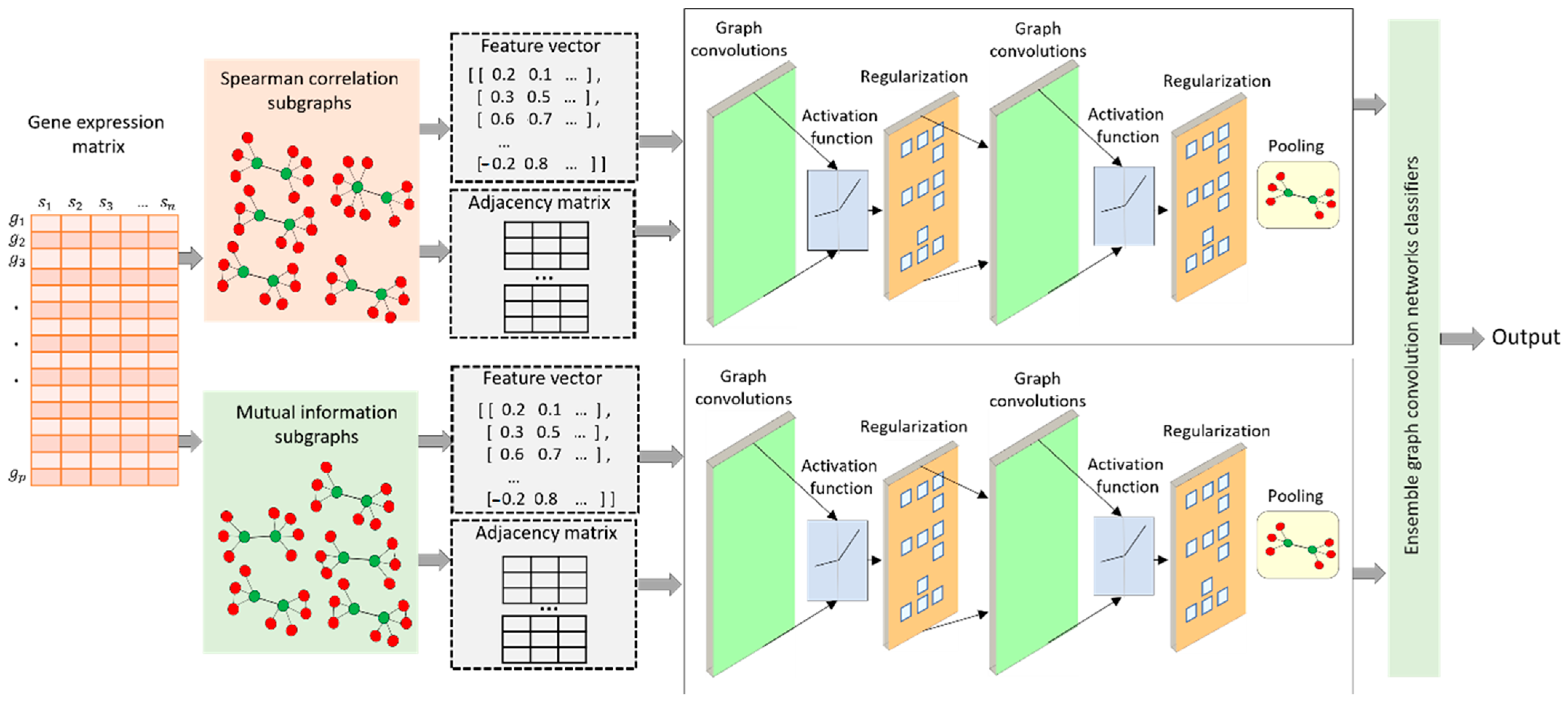
We introduce the EGRC framework, illustrated in Figure 2, to classify subgraphs as positive or negative. The four phases make up the entire EGRC process: (1) constructing noisy skeletons; (2) extracting enclosed subgraphs; (3) constructing node features in each subgraph; and (4) building ensemble GCN classifiers.

2.2.1. Creating Noisy Initial Skeletons

To grasp the input’s local structure, we employ heuristic methods to deduce connections between transcription factors (TFs) and their target genes using gene expression data from training and testing datasets. This research applies commonly used techniques like Spearman’s correlation and mutual information as heuristics to establish edges between nodes. Despite the limitations inherent in existing heuristic methods, the edges inferred from them may contain noise. However, incorporating these links as an initial framework provides valuable guidance for the training process. Initially, we construct GRN′ as a noisy skeleton inferred from gene expression data, comprising a total of z noisy skeletons G R N i = <T, G, L i > where i [ 1 , z ] are created from z empirical functions. In each heuristic function f i T , G , the adjacent matrix ( M T , G ) is defined as in Equation (1):
M T , G = 1 , f i T , G > = t h r e s h o l d i 0 , f i T , G < t h r e s h o l d i
The thresholds used in Spearman’s correlation and the mutual information function are 0.8 and 0.5, respectively.

2.2.2. Extracting Enclosed Subgraphs

At the initial approximation of the graph topology G R N i , we anticipate identifying most transcription factor (TF) and target gene couples through co-expression. This is particularly relevant as these pairs are inherently unlabeled and lack known regulatory information. For each known regulatory pair, denoted as t ∈ [6] and g ∈ {G} and (t, g), (t, t) ∈ L, we extract a subgraph S u b i ( t , g ) + that includes the known regulatory pairs and their 1-hop neighbors on the noisy skeleton G R N i as positive subgraphs. Simultaneously, we arbitrarily select tT and g ∈ {G}, (t, g), (t, t) ∉ L and obtain a subgraph S u b i ( t , g ) ; these pairs and their 1-hop neighbors are contained on the noisy skeleton G R N i as negative subgraphs.

2.2.3. Constructing Node Features in Each Subgraph

Every node within the gene regulatory network (GRN) carries valuable information, unveiling its biological roles as either a transcription factor (TF) or a target gene. Node features are constructed using two broad categories of features: explicit features and structural embeddings. Explicit features are computed using the gene expression vector E i of gene i, i ∈{t, g}. It includes the mean (μ), standard deviation (σ), and quantiles of expression values Q1, Q2, and Q3, as defined in Equation (2). Additionally, we designate Q0 as the minimum expression value and Q4 as the maximum expression value.
Q u a n t i l e   P e r c e n t a g e z = Q z + 1 Q z Q 4 Q 0 ,   z { 0 , 1 , 2 , 3 }
Structural embedding features adopt the shape of graph embeddings, which are a learned continuous representation of features for network nodes. To accomplish this, Node2vec is utilized to transform nodes into a low-dimensional space of features, optimizing the likelihood of preserving the node network neighborhoods [27]. Going beyond explicit features, graph embeddings encapsulate the topological structure of networks, capturing the various connectivity patterns within them. Ultimately, we concatenate the graph embeddings with the explicit features to construct the node feature vectors.

2.2.4. Constructing Ensemble GCN Classifiers

Utilizing the subgraph and its associated node features as input, we construct a graph convolutional network employing various pooling layers to categorize the subgraphs into positive and negative graphs.
Graph neural networks (GNNs) are a category of neural networks proposed for effectively processing graph-structured data. Their popularity in graph analysis has surged recently, largely owing to their remarkable performance [28]. These networks function based on pairwise message passing, allowing for graph nodes to continuously enhance their representations by exchanging information with neighboring nodes [29]. Within GNNs, graph convolutional network models emerge as a subclass that leverages the inherent graph structure. These models employ convolutional operations to aggregate node information from the surrounding neighborhoods [30]. They directly manipulate graphs and utilize their structural information. Furthermore, due to their potent ability to learn graph representations, GCNs have demonstrated outstanding performance across a broad spectrum of tasks and applications [31].
According to the general principle of GCNs, each node’s feature vector is constructed by gathering feature data from its neighbors and the node’s features. This process is then replicated across all nodes. Following that, these features are input into a graph convolutional network. The fundamental elements of the GCN include the convolutional and pooling layers, enabling direct interaction with the graph data structure [30].
The pooling layer functions as a nonlinear down-sampling operation, diminishing the dimensionality of feature representation. This reduction contributes to lower computation costs and a smaller memory footprint and mitigates the risk of overfitting and a decrease in the number of learned parameters [32]. Consequently, pooling facilitates the implementation of deeper networks in practice and is a measure against overfitting. Moreover, pooling exhibits desirable translation-invariant properties in various applications. While there have been debates about the use of pooling in CNNs lately, it still maintains its popularity. While there are plenty of suggested graph convolutional layers for graph convolutional networks (GCNs), the variety of proposed pooling layers is entirely restricted [33]. Despite this constraint, strategic graph pooling holds promise as a direction for enhancing the model. There are two typical kinds of pooling approaches: (1) clustering-based methods, which cluster the original graph into subgraphs at each time of pooling, such as the DiffPool and MinCutPool method; and (2) sorting-based methods, which rank nodes and only retain them partially during pooling, such as the SAGPool method [34]. In this study, we present three recent graph pooling algorithms:
(i) Differentiable Pooling (DiffPool) [30] is notable as a differentiable graph pooling module created to obtain hierarchical representations of graphs by aggregating nodes through multiple pooling layers. Experiment results for DiffPool demonstrate an average accuracy enhancement for graph classification, ranging from 5% to 10%, compared to other pooling methods [35]. DiffPool employs a learned assignment matrix S ( l ) R n 1 x n l + 1 , updating the graph signal and topology through the following process:
X ( l + 1 ) = S ( l ) T Z ( l )
A ( l + 1 ) = S ( l ) T A ( l ) S ( l )
The matrix S ( l ) captures how nodes at layer l are linked to clusters at the next layer, l + 1. Each column in S ( l ) represents a cluster in the subsequent layer, while each row represents a node or cluster at layer l. In simpler terms, S ( l ) provides a flexible assignment for nodes at layer l to clusters in the next simplified layer, l + 1.
Once S ( l ) is calculated, we label the input adjacency matrix at this layer as A ( l ) and the input node embedding matrix as Z ( l ) . Using these inputs, the DIFFPOOL ( A ( l + 1 ) , X ( l + 1 ) ) = DIFFPOOL( A ( l ) , X ( l ) ) process refines the input graph, creating a fresh coarsened adjacency matrix A ( l + 1 ) and a new set of embeddings X ( l + 1 ) for each node or cluster node within this refined graph. In Equation (3), the node embeddings Z ( l ) become amalgamated based on the cluster assignments S ( l ) , generating embeddings for each of the n l + 1 clusters. Similarly, Equation (4) employs the adjacency matrix A ( l ) to formulate a condensed adjacency matrix representing the connection strength between each pair of clusters.
Through the utilization of Equations (3) and (4), the fundamental idea behind the DIFFPOOL layer is graph coarsening. This means that the adjacency matrix A ( l + 1 ) of the following layer signifies a refined graph with n l + 1 nodes or cluster nodes. Each cluster node in this newly refined graph aligns with a cluster of nodes at layer l. Consequently, DiffPool is recognized as a hierarchical approach to learning graph representations, grounded in the concept of clustered nodes.
(ii) Self-Attention Graph Pooling (SAGPool) [36] surfaces as a method for graph pooling that delves into hierarchical graph structures within graph neural networks (GNNs). SAGPool enables pooling while considering both node attributes and the overall graph topology. This method incorporates a self-attention mechanism that distinguishes between nodes to be dropped and those to be retained [9]. Beyond the consideration of graph topology, SAGPool computes attention scores and node characteristics through graph convolution, resulting in hierarchical graph representation learning based on sorted nodes [37]. Moreover, as evidenced by the experimental findings, SAGPool showcases enhanced performance in graph classification on benchmark datasets with a modest parameter count. According to the authors, SAGPool was introduced as a pioneering approach utilizing self-attention for top-notch graph pooling, presenting benefits over other methods outlined in [31,33].
y = G N N ( X l , A l )
i = t o p k ( y )
X ( l + 1 ) = X ( l ) t a n h ( y ) i
A l + 1 = A i , i ( l )
Equation (5) represents the graph neural network (GNN) operation. It takes the node features X l and the adjacency matrix A l at layer l as input and produces the attention scores y for the nodes. Next, as Equation (6) mentioned, it selects the indices of the top k nodes based on the attention scores y. These are the nodes that will be retained after pooling. Then in Equation (7), X l + 1   is the node feature matrix for the next layer. The operation involves taking the node features X ( l ) and performing an element-wise multiplication (denoted by ⊙) with the hyperbolic tangent of the attention scores y for the selected top k nodes ( y i ). The tanh function ensures that the attention scores are scaled between −1 and 1, providing a non-linear transformation. Finally, in Equation (8) the adjacency matrix for the next layer l + 1 is updated. It extracts the submatrix of A(l) corresponding to the top k nodes selected in Equation (6). This submatrix represents the connections among the retained nodes.
(iii) MinCut Pooling is a method employed in graph neural networks for data aggregation. In graph neural networks, pooling serves the goal of roughly partitioning the graph, efficiently diminishing its intricacy and dimensionality. This, in turn, facilitates a more comprehensive understanding or interpretation of the graph’s features or components. MinCut Pooling is one of the pooling methods that seeks to divide the graph into multiple non-overlapping subgraphs or clusters [38]. This method is formulated as an optimization problem to minimize the weights of the edges severed during partitioning while maximizing the sum of internal degrees within each resulting subgraph. This method attempts to preserve the most significant and tightly connected nodes within each subgraph while reducing the connections between subgraphs. The advantage of such an approach is maintaining the original graph’s structure and essential characteristics [39], even as its size is decreased. This improves the efficacy of graph neural networks on various tasks [40], including node classification, graph classification, etc.
S = s o f t m a x ( G N N ( X l , A l )
A p o o l = S T A ˇ S ;   X p o o l = S T X
In the MinCut Pooling method, Equation (9) defines the generation of the cluster assignment matrix S using a graph neural network (GNN). The GNN takes the node features X l and the adjacency matrix A l at layer l as inputs, and the resulting output is passed through a softmax function to produce S, where each element represents the probability of a node being assigned to a specific cluster. Equation (10) shows the pooling results: A p o o l = S T A ^   S is the refined adjacency matrix, and X p o o l = S T X is the pooled node feature matrix. Here, A ^ represents the normalized adjacency matrix. These operations project the original graph structure and node features into a reduced space defined by the clusters, effectively summarizing the graph into fewer nodes with aggregated connections and features.

2.3. Performance Evaluation Metrics

EGRC is a useful subgraph extraction tool designed to work with diverse datasets, including E. coli, S. cerevisiae, and in silico datasets. It leverages these datasets to extract subgraphs, which are then classified as positive or negative. The classification procedure entails building a graph convolution network with diverse pooling layers. We utilize a training set and a distinct dataset as the test set to assess the models’ performance.
In assessing the efficiency of subgraph classification, our study employs two pivotal evaluation metrics: the Precision–Recall (PR) curve and the Receiver Operating Characteristic (ROC) curve. The PR curve, initially introduced by Jesse Davis in 2006 [41], alongside the ROC curve, credited to Yang Shengping’s work in 2017 [42], is foundational in providing a multifaceted evaluation of our algorithm’s performance. Utilizing these metrics facilitates a nuanced understanding of the algorithm’s effectiveness in identifying accurate positives within varied subgraph classifications.
Specifically, the PR curve emerges as a critical tool in elucidating the algorithm’s operational precision and recall dynamics. Precision, defined as the proportion of true positive predictions in relation to all positive predictions made, and recall, the measure of the algorithm’s ability to correctly identify all relevant instances, are juxtaposed at various threshold levels. This comparison yields invaluable insights into the trade-offs between precision and recall, presenting a detailed picture of the algorithm’s performance under different operational conditions. By meticulously analyzing these trade-offs, the PR curve aids in pinpointing the optimal balance where both precision and recall are maximized, thereby enhancing the algorithm’s efficiency in classifying subgraphs accurately.
Moreover, the PR curve’s significance is amplified when the balance between precision and recall becomes critical to the algorithm’s application. For instance, prioritizing recall may be necessary in applications where missing a relevant subgraph classification has high stakes. Conversely, improving precision becomes paramount in contexts where the cost of false positives is substantial. The PR curve’s ability to detail these aspects provides a comprehensive framework for evaluating the algorithm’s performance beyond mere accuracy metrics.
On the other hand, the ROC curve offers a different perspective by mapping the true positive rate (sensitivity) against the false positive rate (1-specificity). This metric is particularly useful in understanding how well the algorithm discriminates between different classes under varying threshold settings. Together, the PR and ROC curves furnish a robust evaluation framework, enabling us to discern the algorithm’s effectiveness not only in terms of its accuracy but also in its practical applicability across various operational contexts .

3. Results

This section comprises several main components. Firstly, we present the outcomes obtained by employing three distinct pooling layers in graph convolutional networks for inferring gene regulatory networks (GRNs). Through thorough analysis, we evaluate and compare the results achieved by these pooling layers, providing insights into their individual contributions to GRN inference. Next, utilizing the best pooling method, we assemble the top-performing results obtained from Spearman’s correlation and mutual information. By combining these results, we propose a final method that leverages the strengths of both correlation measures. This ensemble approach aims to enhance the accuracy and reliability of the GRN inference process. Lastly, we conduct a comparative analysis where EGRC is benchmarked against other relevant methods documented in the existing literature [43]. By undertaking this comparison, we assess EGRC’s performance in relation to similar methods, thereby gaining a deeper understanding of its effectiveness and potential advantages in the context of GRN inference.

3.1. Comparing GRN Using Different Pooling Methods

A comparison of three pooling methods, MinCutPool, DiffPool, and SAGPool, has been carried out regarding their AUROC and AUPR performance. These methods were integrated into a graph convolution network to classify subgraphs extracted based on a Spearman correlation and mutual information.
Table 2 presents a comprehensive performance comparison among MicutPooling, DiffPooling, and SAGPool within the framework of a graph convolutional network, focusing on their efficacy in analyzing the in silico dataset. Among these, the SAGPooling layer distinguishes itself by demonstrating superior performance. Specifically, when leveraging a subgraph based on a Spearman correlation, SAGPooling achieves notable results with an AUROC of 0.834 and an AUPR of 0.623. Further, employing a mutual information-based subgraph attains an AUROC of 0.793 and an AUPR of 0.476. A combined analysis of both skeleton types further elevates its performance, yielding an impressive AUROC of 0.835 and an AUPR of 0.612.
The methodological insights extend across different pooling methods. For DiffPool, the Spearman correlation (SP) struggles with class differentiation, as evidenced by its lower AUROC and AUPR scores (0.600 and 0.287, respectively). On the other hand, mutual information (MI) significantly outperforms SP, with scores of 0.834 in AUROC and 0.556 in AUPR, indicating superior predictive accuracy. The ensemble approach, blending SP and MI, though slightly behind MI’s solo performance, still posts commendable scores of 0.807 in AUROC and 0.500 in AUPR, showcasing its effective adaptability. MinCutPool observations reveal a similar trend, with MI outperforming SP and the ensemble approach closely trailing MI, suggesting that integrating SP and MI offers enhanced performance levels. In the case of SAGPool, SP’s performance in certain metrics either rivals or surpasses the ensemble, pointing to instances where SP alone may be more effective. Although MI’s performance is slightly lower than SP and the ensemble, it varies depending on the context, indicating its nuanced impact.
Across various pooling methods and metrics, the ensemble strategy (SP + MI) consistently delivers robust performances, illustrating its balanced and resilient nature. This synergy likely benefits from the combined strengths of SP and MI, minimizing the risk of specific scenario underperformance and enhancing the model’s overall reliability and applicability. The analysis highlights the ensemble approach’s effectiveness in merging SP and MI to achieve a consistently strong and balanced performance. Despite MI often outperforming SP directly, the combined strategy effectively enhances the model’s efficacy, particularly in achieving an optimal balance between classification accuracy (AUROC) and positive class precision (AUPR). The ensemble method’s adaptability and reliability across different pooling methods and metrics underscore its potential to refine predictive modeling, especially within complex in silico datasets.
In Table 3, our analysis extends to the S. cerevisiae dataset, highlighting the effectiveness of various pooling techniques, with a particular focus on the SAGPooling layer’s performance across different evaluation metrics. The table contrasts the performances of three pooling methods—DiffPool, MinCutPool, and SAGPool—utilizing a Spearman correlation, mutual information, and an ensemble approach that combines both the Spearman correlation and mutual information. This comparison is grounded in two key performance indicators: the Area Under the Receiver Operating Characteristic curve (AUROC) and the Area Under the Precision–Recall curve (AUPR).
Integrating a Spearman correlation and mutual information, the ensemble approach consistently demonstrates superior efficacy, offering compelling evidence of its advantage. For instance, within the SAGPooling analysis, employing Spearman correlation alone yields an AUROC of 0.834 and an AUPR of 0.818. Meanwhile, utilizing mutual information as a standalone measure results in closely matched AUROC and AUPR scores of 0.807. The integration of these two methodologies—Spearman correlation and mutual information—enhances performance, achieving an AUROC of 0.854 and maintaining an AUPR of 0.807.
Our comprehensive assessment underscores that while individual metrics like a Spearman correlation or mutual information offer valuable insights, combined use through an ensemble strategy markedly improves performance. This is particularly evident in the MinCutPool and SAGPool analyses, where the ensemble method outstrips the individual performances of the Spearman correlation and mutual information, delivering the highest AUROC and AUPR scores. Such outcomes firmly establish the ensemble approach as a robust method that leverages the strengths of both Spearman correlation and mutual information, culminating in enhanced predictive accuracy and reliability across different pooling methods.
This synthesis of results from Table 3 clearly illustrates the ensemble method’s superior performance over the singular use of a Spearman correlation or mutual information. It effectively harnesses each method’s unique advantages, leading to more effective and generally superior performance across diverse pooling methods and evaluation metrics. Therefore, the ensemble approach emerges as a more beneficial strategy for analyzing complex datasets, especially when aiming for the highest performance accuracy and reliability levels.
Table 4 provides a detailed comparative analysis of various pooling methods applied to the E. coli dataset, specifically focusing on their performance metrics, AUROC and AUPR. This analysis evaluates three pooling methods, DiffPool, MinCutPool, and SAGPool, across three different data representation approaches: a Spearman correlation (SP), mutual information (MI), and an ensemble approach that synergizes SP and MI. The table meticulously reports the AUROC and AUPR values for each method and approach, with superior scores distinctly highlighted. The ensemble approach, combining SP and MI, emerges as a robust performer, often outmatching or closely rivaling the individual performances of SP or MI in terms of AUPR. This pattern underscores the ensemble’s efficacy in drawing upon the strengths of both SP and MI to yield enhanced or equivalent outcomes compared to the best-performing individual method.
The ensemble approach’s relative superiority, particularly noted in the context of AUPR, is significant for applications where precision and recall are paramount, such as in imbalanced datasets. This advantage stems from the ensemble’s balanced and comprehensive data representation, marrying the rank sensitivity of Spearman correlation with the non-linear dependency detection afforded by mutual information. This blend addresses the limitations inherent in each approach and capitalizes on their collective strengths to boost overall model performance.
The analysis presented in Table 4 underscores the ensemble approach’s (SP + MI) distinct advantage in handling the E. coli dataset across varied pooling methods. Although the ensemble might not always lead in AUROC, its consistent uplift or competitive parity in AUPR across all pooling methods solidifies its value. The ensemble’s ability to outperform or match the best individual methods’ performances highlights its potential as the preferred choice for scenarios where precision and recall are critical, effectively leveraging the integrated strengths of SP and MI to optimize model performance.
Upon confirming that the combined use of a Spearman correlation and mutual information (SP + MI) as an ensemble method leads to superior outcomes, we conducted a detailed comparison of different pooling layers—namely DiffPool, MinCutPool, and SAGPool—across several datasets, as outlined in Table 5. This comparison reveals the impact of implementing the ensemble strategy within various pooling layers for datasets such as in silico, S. cerevisiae, and E. coli, with a focus on two critical metrics: the Area Under the Receiver Operating Characteristic curve (AUROC) and the Area Under the Precision–Recall curve (AUPR). These metrics illustrate the ensemble method’s performance in each pooling layer.
The patterns observed in Table 5 are striking, showing that SAGPool, when paired with the SP + MI ensemble approach, consistently exceeds the performance of other pooling layers across all datasets examined. For example, within the in silico dataset, SAGPool achieves AUROC and AUPR scores of 0.835 and 0.612, respectively, outperforming the scores obtained by both DiffPool and MinCutPool using the same ensemble method. This trend of SAGPool’s dominance continues across the S. cerevisiae and E. coli datasets, where it secures the highest AUROC and AUPR scores, solidifying its lead.
These results highlight SAGPool’s exceptional ability to leverage the combined strengths of a Spearman correlation and mutual information effectively. This pooling layer demonstrates superior adaptability to the nuances of different datasets and enhances the predictive accuracy and reliability of the models. SAGPool’s consistently superior performance across a variety of datasets underscores its robustness and efficiency in processing complex biological data, making it the preferred choice for researchers seeking the highest quality in computational analysis.
In summary, Table 5 convincingly demonstrates that using the SAGPool layer in conjunction with the SP + MI ensemble approach significantly surpasses other pooling layers in various datasets. This is evidenced by the highest AUROC and AUPR scores, signifying SAGPool’s superior capability in making accurate and reliable predictions. Therefore, our study conclusively positions the ensemble method with SAGPool as the most effective approach for analyzing complex datasets, emphasizing its importance in the evolution of computational research methodologies.
In addition to performance evaluation, we also compared the execution times of MinCutPool, DiffPool, and SAGPool on the E. coli datasets (Table 6). The findings revealed that SAGPool was faster in execution time than the other methods.
Several reasons can explain the superior performance of SAGPooling over Diffpool and MinCutPool, for instance,
-
Selective pooling: SAGPooling employs a self-attention mechanism to selectively pool a subset of nodes pertinent to the graph’s overall properties. This ability can sometimes lead to improved performance by capturing significant structural features of the graph more effectively than other methods.
-
Adaptability: SAGPooling demonstrates superior adaptability to various graph structures. In contrast to DiffPool and MinCut Pooling, it does not require clustering the graph into a predetermined number of clusters or partitioning it into non-overlapping clusters, affording it greater flexibility.
-
Computational efficiency: SAGPooling is often more computationally efficient than methods like DiffPool or MinCut Pooling, particularly for larger graphs. This efficiency can facilitate the development of more complex or deeper graph convolutional networks (GCNs), potentially enhancing performance.
-
Less information loss: SAGPooling retains the most informative nodes and their connections, reducing information loss during the pooling process compared to other methods. This characteristic may lead to improved representation learning, thereby enhancing performance.
After selecting the best pooling method (SAGPool), we combined the results from Spearman’s correlation network and the mutual information network, which produces useful information for our proposed model. In the subsequent sections, we assess the performance of EGRC in comparison to other similar methods, including LEAP, GENIE3, GRNBoost2, PIDC, and PPCOR.

3.2. Analytical Comparison with Existing Approaches

To evaluate the effectiveness of EGRC, we replicated five benchmarking techniques stated in Pratapa et al., 2020—specifically, LEAP [44], GENIE3 [45], GRNBOOST2 [46], PIDC [47], and PPCOR [48] —utilizing three datasets from DREAM5 [43] in silico, S. cerevisiae, and E. coli. The benchmarking methods chosen for comparison with EGRC on the DREAM5 dataset have been carefully selected to encompass diverse approaches to gene regulatory network inference. Each method offers unique strengths and perspectives, making them suitable for comprehensive evaluation.
LEAP constructs gene co-expression networks from single-cell RNA-sequencing data by leveraging pseudo-time ordering to capture dynamic changes in gene expression over time. This approach is particularly valuable for understanding temporal dynamics in gene regulation, which aligns well with the goals of the EGRC method. We can assess how well EGRC captures temporal gene expression patterns by comparing it with LEAP. LEAP effectively captures dynamic co-expression patterns over time, providing insights into the temporal progression of cellular states. GENIE3 infers gene regulatory networks using ensemble methods of tree-based regression, where each gene’s expression is predicted from the expression of all other genes. This method is known for its robustness and ability to identify regulatory relationships based on feature importance scores. Comparing EGRC with GENIE3 allows us to evaluate the efficacy of EGRC in capturing regulatory relationships in a robust manner. Ensemble methods in GENIE3 enhance the accuracy and robustness of inferred regulatory networks.
GRNBoost2 employs gradient-boosting machines to predict regulatory interactions, offering an efficient and scalable approach. Its iterative decision tree-building process is designed to handle large datasets effectively. By including GRNBoost2 in the comparison, we can assess the scalability and efficiency of EGRC in inferring gene regulatory networks. GRNBoost2 is highly efficient and scalable, making it suitable for large datasets. PIDC infers gene networks by quantifying multivariate information measures, focusing on identifying non-linear dependencies and direct interactions between genes. This method’s ability to capture non-linear relationships is crucial for a comprehensive evaluation of EGRC, which aims to uncover complex regulatory interactions. PIDC’s strength lies in its ability to capture non-linear dependencies and direct interactions, providing a nuanced view of gene regulatory networks, while PPCOR calculates partial correlation coefficients to infer gene regulatory networks by controlling for the effects of other variables. This method provides a direct measure of the relationships between genes, making it a valuable benchmark for assessing the precision of EGRC in identifying direct regulatory interactions. PPCOR’s strength is in directly measuring relationships by controlling other variables, ensuring an accurate identification of the regulatory interactions.
Regarding the datasets chosen for comparison, in silico datasets offer controlled complexity, allowing researchers to design varying levels of complexity from simple linear interactions to highly complex non-linear dependencies, with the ability to control the number of genes, interaction density, and relationship types. Noise can be systematically introduced and controlled to simulate different experimental conditions, enabling the testing of inference methods’ robustness. Being synthetic, these datasets may lack the biological variability and unexpected patterns found in real-world data, but they benefit from known ground truth, making accuracy evaluation straightforward.
In contrast, S. cerevisiae, a model organism in genetics, presents a highly complex gene regulatory network with numerous well-studied pathways and interactions, high dimensionality, and non-linear dependencies, contributing to the complexity of network inference. These datasets also contain biological noise and experimental variability. Similarly, E. coli has a moderately complex gene regulatory network with well-annotated interactions, influenced by interactions among many genes and regulatory elements, and is subject to biological noise and variability from experimental conditions and genetic diversity. The presence of direct and indirect gene interactions further complicates network inference, and although there is substantial knowledge of E. coli’s gene network, it remains incomplete with potential unknown interactions.
By selecting these methods and using these datasets, we ensure a comprehensive and rigorous benchmarking process, allowing us to evaluate the performance of EGRC from multiple perspectives. This includes link predictive accuracy, robustness, and resilience. This holistic approach provides a thorough comparison, highlighting the strengths and potential areas for improvement of the EGRC method.
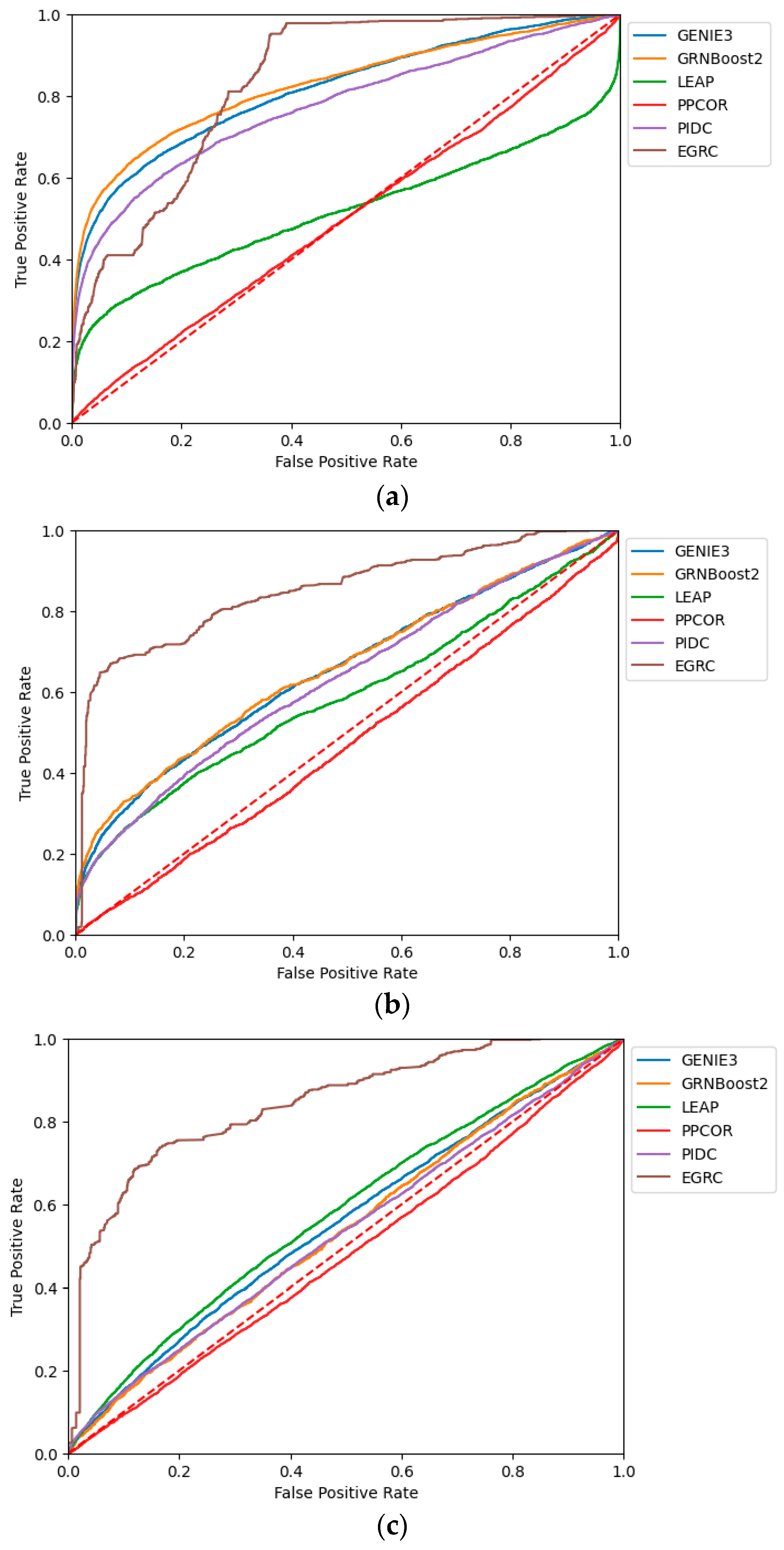
Figure 3 and Figure 4 illustrate the AUROC and AUPRC performance of the assessed techniques across these three simulated DREAM5 datasets. Notably, EGRC consistently surpasses the other methods on all three datasets. Figure 3a shows a distinct trend while evaluating the in silico dataset. The initial AUROC value is relatively low but exhibits gradual improvement over time. To assess the proposed method on the in silico dataset, we utilized the E. coli dataset as the training dataset. The E. coli dataset comprises real data, whereas the in silico dataset is generated synthetically. Figure 3a highlights the initial difficulty our model faced in comprehending the relevant features within the data. However, as the training process advanced, the model successfully learned to extract more meaningful and informative features from the input data, improving its predictive performance. This feature learning process significantly contributed to the rapid enhancement of the AUROC score.
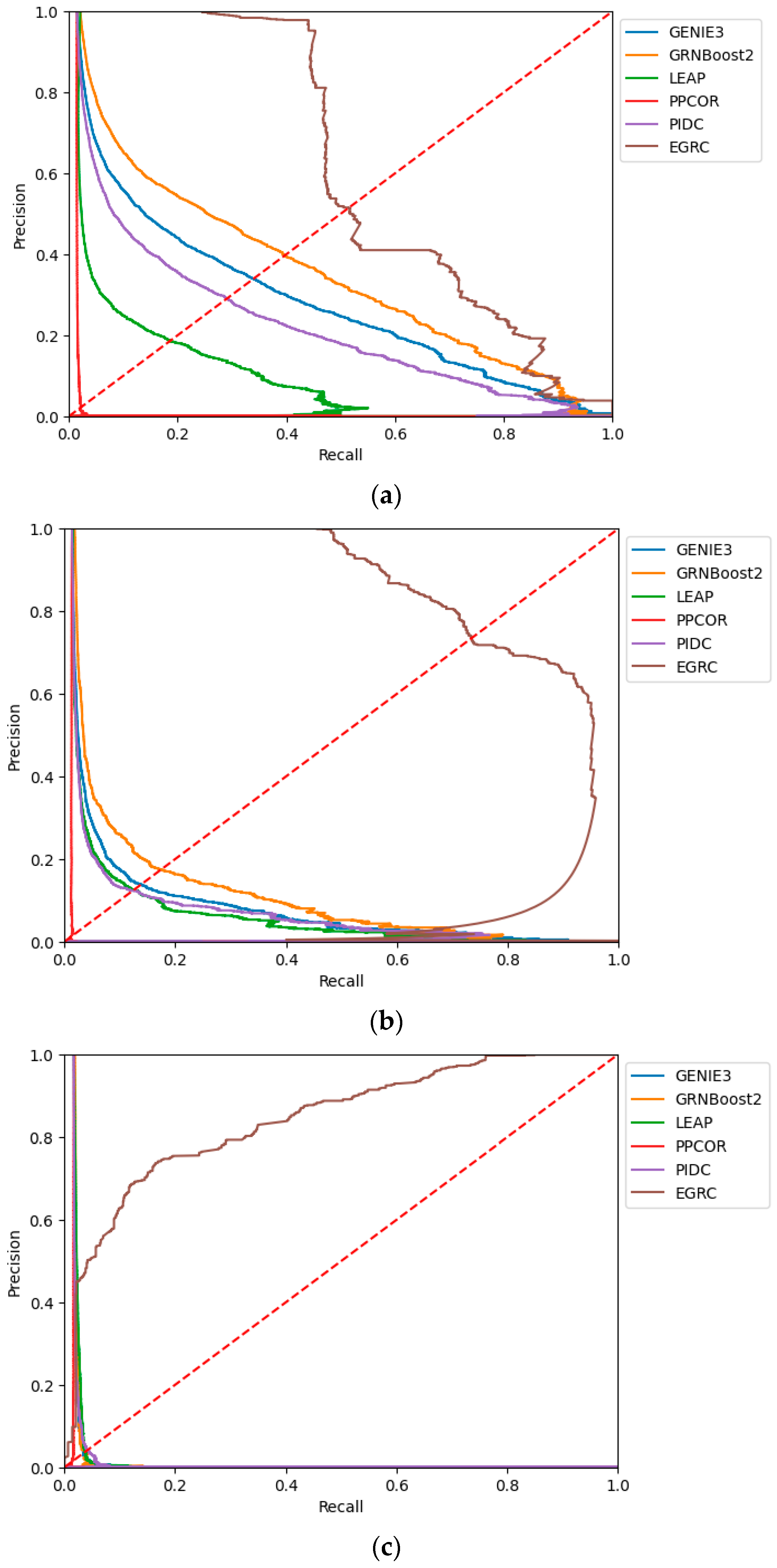
Figure 4 presents the comparative Precision–Recall curves for various GRN prediction algorithms across three DREAM5 datasets: (a) in silico, (b) E. coli, and (c) S. cerevisiae. EGRC consistently outperforms other methods, maintaining high precision and recall, especially in real-world datasets like E. coli and S. cerevisiae, demonstrating its robustness in handling complex gene regulatory networks with significant noise. GENIE3 and GRNBoost2 also show strong performance with balanced precision and recall, though they are slightly less effective in noisy environments. LEAP, PPCOR, and PIDC exhibit more variable performance, particularly with real-world datasets due to lower precision and recall. Overall, EGRC’s superior performance highlights its capability to accurately detect true regulatory links with minimal false positives across diverse datasets.
Our observations highlight an enhancement compared to five other methods, namely LEAP [44], GENIE3 [45], GRNBOOST2 [46], PIDC [47], and PPCOR [48]. EGRC exhibited superior performance assessed to the commonly utilized technique, GENIE3.
In addition, we compared the performance of five benchmark methods—LEAP, GENIE3, GRNBoost2, PIDC, and PPCOR—against EGRC using three criteria: link predictive accuracy, robustness, and resilience.
Link predictive accuracy evaluates a method’s ability to correctly predict the presence or absence of regulatory links between genes. This is critical for identifying regulatory relationships and is measured using standard performance metrics such as the Area Under the Receiver Operating Characteristic curve (AUROC) and the Precision–Recall Curve (AUPR). The comparative analysis shows LEAP performs well in E. coli and S. cerevisiae datasets but less effectively in in silico datasets. GENIE3 demonstrates high accuracy, while GRNBoost2 exhibits medium to high accuracy due to its ensemble learning approach. PIDC achieves good accuracy, excelling in identifying non-linear dependencies in the in silico dataset, and PPCOR also shows good accuracy, relying on partial correlations in the in silico dataset.
Robustness refers to a method’s ability to maintain performance across different datasets and conditions, ensuring consistent performance across diverse datasets. This was assessed by testing each method on multiple datasets with different characteristics, including in silico, E. coli, and S. cerevisiae. LEAP’s reliance on pseudo-time ordering makes it less robust across different dataset types. GENIE3 is highly robust and performs well across diverse datasets. GRNBoost2 is moderately robust, with performance varying depending on dataset characteristics. PIDC’s robustness is low and influenced by data complexity, while PPCOR also exhibits low robustness and struggles with larger networks.
Resilience measures a method’s ability to handle errors, missing data, or unexpected variations in the data. This criterion was evaluated by introducing noise (perturbations) into the datasets, simulating real-world conditions such as those found in the E. coli dataset, where experimental data often contain noise and variability. The results indicate that LEAP is moderately effective in noise mitigation, performing well in specific scenarios but lacking comprehensiveness. GENIE3 shows low noise mitigation, with significant performance drops in noisy data. GRNBoost2 manages noise better than some methods but maintains only medium effectiveness. PIDC excels in noise mitigation due to its use of multivariate measures, while PPCOR handles noise moderately well but is less effective compared to others.
Conversely, EGRC demonstrates superior performance across all three criteria. Its innovative use of Graph Convolution with Self-Attention Graph Pooling enhances link predictive accuracy by capturing complex patterns in gene regulation. Additionally, dual GCN models improve robustness and resilience by effectively classifying ‘Positive’ and ‘Negative’ subgraphs. The combination of Spearman’s correlation and mutual information provides superior noise mitigation by capturing a broader spectrum of gene interactions, making EGRC highly effective even in noisy datasets like E. coli.

4. Conclusions

Within this investigation, we have presented EGRC, a framework crafted to determine the presence of a connection within a subgraph focused on two nodes. A subgraph receives a positive label if associated with a transcription factor (TF) and its corresponding target gene. Conversely, a subgraph without a connection between a TF and its target gene is assigned a negative label.
Through our experimentation, we have pinpointed several factors influencing the predictive capabilities of EGRC concerning gene regulatory networks (GRNs). Deploying an ensemble strategy that fuses various heuristic frameworks empowers us to adeptly address the inherent constraints within individual frameworks. This includes those constructed using Spearman’s correlation coefficient or mutual information, particularly in scenarios with relatively minimal noise levels. This ensemble technique leverages diverse information obtained from different perspectives, including nonlinear correlation and information theory, effectively mitigating noise-related issues. Additionally, training and testing the heuristics enable graph convolution networks (GCNs) to learn the relationship mapping between the heuristics and the actual regulatory connections, thereby enhancing model accuracy and effectiveness.
Furthermore, the pivotal role of graph embedding techniques lies in their adeptness at capturing the innate topological structures of the network, constituting a significant contribution to the realm of link prediction. Beyond extracting regulatory pairs alone, incorporating subgraphs encompassing neighboring nodes provides valuable supplementary information. Node2vec, as a graph embedding technique, generates a more accurate and precise representation of the graph, thereby enhancing link prediction capabilities. Effectively extracting explicit features from gene expression data proves beneficial, considering the critical role of gene expression in deducing gene regulatory networks (GRNs). Features that portray the comprehensive distribution and patterns of input expression—such as z-score, standard deviation, and quantile percentages—elevate the data representation of the EGRC model, leading to enhanced performance.
Lastly, incorporating a graph convolutional network with an enhanced pooling layer, such as the SAGPool technique, significantly augments the performance of the graph classifier. The advanced pooling capabilities of the SAGPool technique allow the network to effectively capture and utilize crucial graph features, resulting in improved classification outcomes. Conducting a thorough comparison, EGRC outshines five benchmark methods (LEAP, GENIE3, GRNBoost2, PIDC, and PPCOR) across three DREAM5 networks. Through the utilization of DREAM5′s in silico data, EGRC exhibits a 0.85% enhancement in AUROC and a notable 74.07% improvement in AUPR compared to the runner-up method (GRNBoost2). For the E. coli dataset, EGRC showcases a remarkable 30.08% surge in AUROC and an outstanding 95.01% boost in AUPR.
EGRC surpasses existing methods in terms of AUROC and AUPR across multiple datasets, demonstrating its robustness and accuracy. Accurate GRN reconstruction aids in identifying key regulatory genes involved in diseases such as cancer and diabetes, supports gene function annotation, and facilitates biomarker discovery for early diagnosis and monitoring. EGRC enhances the understanding of cellular pathways, supports systems biology studies, and advances personalized medicine by enabling tailored treatment plans. Comparing GRNs across species provides insights into the evolutionary conservation and divergence of regulatory mechanisms.
Despite the encouraging outcomes of our methodology, it is crucial to recognize a significant constraint: our dependence on DREAM5 datasets. These datasets, sourced from extensively studied model species and featuring synthetic data, serve as the exclusive benchmark data with empirically validated, gold-standard regulatory relationships. To enhance the EGRC model, future plans involve integrating additional types of biological data, such as epigenetic data, protein–DNA interaction data, and chromatin accessibility data, to improve the accuracy and robustness of GRN inference. Incorporating more sophisticated heuristic methods to generate initial noisy skeletons could enhance the initial approximation of GRN structures. Applying the EGRC framework to a broader range of species beyond model organisms like E. coli and S. cerevisiae, including human and plant datasets, would help validate its generalizability and utility in diverse biological contexts. Encouraging collaboration with experimental biologists to validate the inferred GRNs through laboratory experiments is essential to ensure the practical applicability of the predicted regulatory interactions. Additionally, leveraging methodologies such as kTWAS, which integrates kernel machines with transcriptome-wide association studies, can improve statistical power and reveal novel genes, providing further insights into complex regulatory mechanisms. This integrated approach highlights the necessity for the continual development and validation of computational models to unravel the intricacies of gene regulation and its implications in health and disease.
In summary, the EGRC model holds the potential to accurately deduce gene regulatory networks (GRNs) across a wide array of species, significantly advancing our understanding of biological systems and disease processes.

5. Expanded Discussion on Particular Biological Implications

Our study introduces the Enhanced Graph Representation Convolution (EGRC) method, demonstrating superior performance in predicting gene regulatory networks (GRNs) across multiple datasets. The biological implications of these findings are substantial and multifaceted:
(a)
Identification of Key Regulatory Genes: An accurate reconstruction of GRNs is crucial for identifying key regulatory genes involved in various biological processes and diseases. For instance, our method can help pinpoint transcription factors (TFs) pivotal in cancer progression, metabolic disorders, or developmental processes. By accurately mapping these regulatory relationships, EGRC aids in uncovering potential targets for therapeutic intervention.
(b)
Gene Function Annotation: Understanding gene regulatory interactions enhances gene function annotation. Many genes, especially newly discovered or less studied, have unknown or poorly characterized functions. By identifying regulatory connections, EGRC contributes to predicting the roles of these genes within broader biological pathways, facilitating a deeper understanding of their contributions to cellular functions and organismal development.
(c)
Biomarker Discovery: EGRC’s high precision and recall demonstrated in noisy datasets like E. coli suggest its robustness in handling real-world biological data, which often contain variability. This capability is crucial for biomarker discovery, where identifying reliable molecular signatures for disease diagnosis, prognosis, and monitoring is essential. EGRC’s ability to accurately predict regulatory links can lead to identifying novel biomarkers for early disease detection and personalized medicine.
(d)
Systems Biology and Pathway Analysis: EGRC enhances the understanding of complex cellular pathways by providing detailed maps of gene regulatory interactions. This is particularly valuable in systems biology, where comprehensive models of cellular networks are constructed to understand how various biological components interact and give rise to phenotypic traits. EGRC’s accurate GRN predictions can be integrated into these models, offering insights into pathway dynamics and cellular responses to stimuli.
(e)
Comparative Genomics and Evolutionary Studies: By applying EGRC to datasets from different species, researchers can compare GRNs to explore the evolutionary conservation and divergence of regulatory mechanisms. Understanding these evolutionary aspects can reveal how regulatory networks have adapted to different environmental conditions and evolutionary pressures, shedding light on fundamental biological principles and species-specific adaptations.
(f)
Advancements in Personalized Medicine: The precise prediction of GRNs supports personalized medicine by enabling tailored treatment plans based on an individual’s unique regulatory network profile. This approach can improve therapeutic efficacy and reduce adverse effects by targeting specific regulatory pathways involved in a patient’s disease.
In short, the EGRC model holds significant potential to advance our understanding of biological systems and disease processes. By accurately deducing GRNs across various species, EGRC contributes to identifying regulatory genes, gene function annotation, biomarker discovery, systems biology studies, and personalized medicine. Future enhancements and broader applications of the model will further impact biological research and clinical practice.

Author Contributions

D.M.A. conducted data collection and processing. The experiments were conceived and designed by D.M.A., A.K. and M.T.H. D.M.A. performed the experiments, and D.M.A., A.K. and M.T.H. analyzed the data. M.T.H. contributed reagents, materials, and analysis tools. D.M.A., A.K. and M.T.H. wrote the paper. All authors have read and agreed to the published version of the manuscript.

Funding

The research reported in the paper was partially supported by an Institutional Development Award (IDeA) from the National Institute of General Medical Sciences of the National Institutes of Health under grant number P2O GM103424-21.

Institutional Review Board Statement

Our study uses publicly available datasets from the DREAM5 challenge, including in silico, E. coli, and S. cerevisiae datasets, which do not require ethical approval as they involve computational simulations, bacterial experiments, and yeast research, none of which involve humans or higher animals.

Data Availability Statement

The complete model code, data, and a functional software version of the AGRN tool are freely accessible at https://github.com/DuaaAlawad/EGRC_tool.git accessed on 18 January 2024.

Conflicts of Interest

The authors declare no conflicts of interest.

References

  1. Marbach, D.; Costello, J.C.; Küffner, R.; Vega, N.M.; Prill, R.J.; Camacho, D.M.; Allison, K.R.; Kellis, M.; Collins, J.J.; Stolovitzky, G. Wisdom of crowds for robust gene network inference. Nat. Methods 2012, 9, 796–804. [Google Scholar] [CrossRef] [PubMed]
  2. Mochida, K.; Koda, S.; Inoue, K.; Nishii, R. Statistical and machine learning approaches to predict gene regulatory networks from transcriptome datasets. Front. Plant Sci. 2018, 9, 1770. [Google Scholar] [CrossRef] [PubMed]
  3. Wang, J.; Ma, A.; Ma, Q.; Xu, D.; Joshi, T. Inductive inference of gene regulatory network using supervised and semi-supervised graph neural networks. Comput. Struct. Biotechnol. J. 2020, 18, 3335–3343. [Google Scholar] [CrossRef] [PubMed]
  4. Zhang, J.; Ibrahim, F.; Najmulski, E.; Katholos, G.; Altarawy, D.; Heath, L.S.; Tulin, S.L. Developmental gene regulatory network connections predicted by machine learning from gene expression data alone. PLoS ONE 2021, 16, e0261926. [Google Scholar] [CrossRef] [PubMed]
  5. Lim, N.; Şenbabaoğlu, Y.; Michailidis, G.; d’Alché-Buc, F. OKVAR-Boost: A novel boosting algorithm to infer nonlinear dynamics and interactions in gene regulatory networks. Bioinformatics 2013, 29, 1416–1423. [Google Scholar] [CrossRef]
  6. Alawad, D.M.; Katebi, A.; Kabir, M.W.U.; Hoque, M.T. AGRN: Accurate gene regulatory network inference using ensemble machine learning methods. Bioinform. Adv. 2023, 3, vbad032. [Google Scholar] [CrossRef] [PubMed]
  7. Pirgazi, J.; Khanteymoori, A.R. A robust gene regulatory network inference method base on Kalman filter and linear regression. PLoS ONE 2018, 13, e0200094. [Google Scholar] [CrossRef] [PubMed]
  8. Pirgazi, J.; Khanteymoori, A.R.; Jalilkhani, M. TIGRNCRN: Trustful inference of gene regulatory network using clustering and refining the network. J. Bioinform. Comput. Biol. 2019, 17, 1950018. [Google Scholar] [CrossRef]
  9. Haury, A.-C.; Mordelet, F.; Vera-Licona, P.; Vert, J.-P. TIGRESS: Trustful inference of gene regulation using stability selection. BMC Syst. Biol. 2012, 6, 145. [Google Scholar] [CrossRef]
  10. Margolin, A.A.; Nemenman, I.; Basso, K.; Wiggins, C.; Stolovitzky, G.; Favera, R.D.; Califano, A. ARACNE: An algorithm for the reconstruction of gene regulatory networks in a mammalian cellular context. BMC Bioinform. 2006, 7, S7. [Google Scholar] [CrossRef]
  11. Gillani, Z.; Akash, M.S.H.; Rahaman, M.; Chen, M. CompareSVM: Supervised, Support Vector Machine (SVM) inference of gene regularity networks. BMC Bioinform. 2014, 15, 395. [Google Scholar] [CrossRef] [PubMed]
  12. Kotera, M.; Yamanishi, Y.; Moriya, Y.; Kanehisa, M.; Goto, S. GENIES: Gene network inference engine based on supervised analysis. Nucleic Acids Res. 2012, 40, W162–W167. [Google Scholar] [CrossRef] [PubMed]
  13. Daoudi, M.; Meshoul, S.; Tahi, F. A Machine Learning Approach for Gene Regulatory Network Inference. Int. J. Biosci. Biochem. Bioinform. 2019, 9, 82–89. [Google Scholar]
  14. Turki, T.; Wang, J.T.; Rajikhan, I. Inferring gene regulatory networks by combining supervised and unsupervised methods. In Proceedings of the 2016 15th IEEE International Conference on Machine Learning and Applications (ICMLA), Anaheim, CA, USA, 18–20 December 2016; pp. 140–145. [Google Scholar]
  15. Meyer, P.E.; Kontos, K.; Lafitte, F.; Bontempi, G. Information-theoretic inference of large transcriptional regulatory networks. EURASIP J. Bioinform. Syst. Biol. 2007, 2007, 79879. [Google Scholar] [CrossRef]
  16. Aliferis, C.F.; Statnikov, A.; Tsamardinos, I.; Mani, S.; Koutsoukos, X.D. Local causal and Markov blanket induction for causal discovery and feature selection for classification part I: Algorithms and empirical evaluation. J. Mach. Learn. Res. 2010, 11, 17–234. [Google Scholar]
  17. Mao, G.; Liu, J. An unsupervised deep learning framework for gene regulatory network inference from single-cell expression data. In Proceedings of the 2023 IEEE International Conference on Bioinformatics and Biomedicine (BIBM), Istanbul, Turkey, 5–8 December 2023; pp. 2663–2670. [Google Scholar]
  18. Mordelet, F.; Vert, J.-P. SIRENE: Supervised inference of regulatory networks. Bioinformatics 2008, 24, i76–i82. [Google Scholar] [CrossRef] [PubMed]
  19. Guo, S.; Jiang, Q.; Chen, L.; Guo, D. Gene regulatory network inference using PLS-based methods. BMC Bioinform. 2016, 17, 1–10. [Google Scholar] [CrossRef] [PubMed]
  20. Razaghi-Moghadam, Z.; Nikoloski, Z. Supervised learning of gene-regulatory networks based on graph distance profiles of transcriptomics data. NPJ Syst. Biol. Appl. 2020, 6, 21. [Google Scholar] [CrossRef] [PubMed]
  21. Augustine, J.; Jereesh, A. Gene regulatory network inference: A semi-supervised approach. In Proceedings of the 2017 International conference of Electronics, Communication and Aerospace Technology (ICECA), Coimbatore, India, 20–22 April 2017; pp. 68–72. [Google Scholar]
  22. Wang, Q.; Guo, M.; Chen, J.; Duan, R. A gene regulatory network inference model based on pseudo-siamese network. BMC Bioinform. 2023, 24, 163. [Google Scholar] [CrossRef] [PubMed]
  23. Gan, Y.; Hu, X.; Zou, G.; Yan, C.; Xu, G. Inferring gene regulatory networks from single-cell transcriptomic data using bidirectional rnn. Front. Oncol. 2022, 12, 899825. [Google Scholar] [CrossRef]
  24. Zhao, M.; He, W.; Tang, J.; Zou, Q.; Guo, F. A hybrid deep learning framework for gene regulatory network inference from single-cell transcriptomic data. Brief. Bioinform. 2022, 23, bbab568. [Google Scholar] [CrossRef] [PubMed]
  25. Hu, F.; Zhu, Y.; Wu, S.; Wang, L.; Tan, T. Hierarchical graph convolutional networks for semi-supervised node classification. arXiv 2019, arXiv:190206667. [Google Scholar]
  26. Shang, J.; Ma, T.; Xiao, C.; Sun, J. Pre-training of graph augmented transformers for medication recommendation. arXiv 2019, arXiv:190600346. [Google Scholar]
  27. Palumbo, E.; Rizzo, G.; Troncy, R.; Baralis, E.; Osella, M.; Ferro, E. Knowledge graph embeddings with node2vec for item recommendation. In The Semantic Web: ESWC 2018 Satellite Events: ESWC 2018 Satellite Events, Heraklion, Crete, Greece, June 3–7, 2018, Revised Selected Papers 15; Springer: Berlin/Heidelberg, Germany, 2018; pp. 117–120. [Google Scholar]
  28. Xu, K.; Hu, W.; Leskovec, J.; Jegelka, S. How powerful are graph neural networks? arXiv 2018, arXiv:1810.00826. [Google Scholar]
  29. Zhou, J.; Cui, G.; Hu, S.; Zhang, Z.; Yang, C.; Liu, Z.; Wang, L.; Li, C.; Sun, M. Graph neural networks: A review of methods and applications. AI open 2020, 1, 57–81. [Google Scholar] [CrossRef]
  30. Zhang, S.; Tong, H.; Xu, J.; Maciejewski, R. Graph convolutional networks: A comprehensive review. Comput. Soc. Netw. 2019, 6, 11. [Google Scholar] [CrossRef] [PubMed]
  31. Kipf, T.N.; Welling, M. Semi-supervised classification with graph convolutional networks. arXiv 2016, arXiv:1609.02907. [Google Scholar]
  32. Sun, M.; Song, Z.; Jiang, X.; Pan, J.; Pang, Y. Learning pooling for convolutional neural network. Neurocomputing 2017, 224, 96–104. [Google Scholar] [CrossRef]
  33. Diehl, F. Edge contraction pooling for graph neural networks. arXiv 2019, arXiv:1905.10990. [Google Scholar]
  34. Mesquita, D.; Souza, A.; Kaski, S. Rethinking pooling in graph neural networks. Adv. Neural Inf. Process. Syst. 2020, 33, 2220–2231. [Google Scholar]
  35. Ying, Z.; You, J.; Morris, C.; Ren, X.; Hamilton, W.; Leskovec, J. Hierarchical graph representation learning with differentiable pooling. In Proceedings of the Advances in Neural Information Processing Systems 31, Montréal, QC, Canada, 3–8 December 2018. [Google Scholar]
  36. Lee, J.; Lee, I.; Kang, J. Self-attention graph pooling. In Proceedings of the International Conference on Machine Learning, Long Beach, CA, USA, 10–15 June 2019; pp. 3734–3743. [Google Scholar]
  37. Ranjan, E.; Sanyal, S.; Talukdar, P. Asap: Adaptive structure aware pooling for learning hierarchical graph representations. In Proceedings of the AAAI Conference on Artificial Intelligence, New York, NY, USA, 7–12 February 2020; pp. 5470–5477. [Google Scholar]
  38. Bianchi, F.M.; Grattarola, D.; Alippi, C. Mincut pooling in graph neural networks. In Proceedings of the ICLR 2020 Conference, Addis Ababa, Ethiopia, 27–30 April 2019. [Google Scholar]
  39. Bianchi, F.M.; Grattarola, D.; Alippi, C. Spectral clustering with graph neural networks for graph pooling. In Proceedings of the International Conference on Machine Learning, Vienna, Austria, 12–18 July 2020; pp. 874–883. [Google Scholar]
  40. Grattarola, D.; Zambon, D.; Bianchi, F.M.; Alippi, C. Understanding pooling in graph neural networks. IEEE Trans. Neural Netw. Learn. Syst. 2022, 35, 2708–2718. [Google Scholar] [CrossRef] [PubMed]
  41. Davis, J.; Goadrich, M. The relationship between Precision-Recall and ROC curves. In Proceedings of the 23rd International Conference on Machine Learning, Pittsburgh, PA, USA, 25–29 June 2006; pp. 233–240. [Google Scholar]
  42. Shengping, Y.; Gilbert, B. The receiver operating characteristic (ROC) curve. Southwest Respir. Crit. Care Chron. 2017, 5, 34–36. [Google Scholar]
  43. Pratapa, A.; Jalihal, A.P.; Law, J.N.; Bharadwaj, A.; Murali, T. Benchmarking algorithms for gene regulatory network inference from single-cell transcriptomic data. Nat. Methods 2020, 17, 147–154. [Google Scholar] [CrossRef]
  44. Specht, A.T.; Li, J. LEAP: Constructing gene co-expression networks for single-cell RNA-sequencing data using pseudotime ordering. Bioinformatics 2017, 33, 764–766. [Google Scholar] [CrossRef]
  45. Huynh-Thu, V.A.; Irrthum, A.; Wehenkel, L.; Geurts, P. Inferring regulatory networks from expression data using tree-based methods. PLoS ONE 2010, 5, e12776. [Google Scholar] [CrossRef] [PubMed]
  46. Moerman, T.; Aibar Santos, S.; Bravo González-Blas, C.; Simm, J.; Moreau, Y.; Aerts, J.; Aerts, S. GRNBoost2 and Arboreto: Efficient and scalable inference of gene regulatory networks. Bioinformatics 2019, 35, 2159–2161. [Google Scholar] [CrossRef] [PubMed]
  47. Chan, T.E.; Stumpf, M.P.; Babtie, A.C. Gene regulatory network inference from single-cell data using multivariate information measures. Cell Syst. 2017, 5, 251–267. [Google Scholar] [CrossRef]
  48. Kim, S. Ppcor: An R package for a fast calculation to semi-partial correlation coefficients. Commun. Stat. Appl. Methods 2015, 22, 665. [Google Scholar] [CrossRef]
Figure 1. Noisy skeletons derived from Spearman’s correlation generate two subgraphs: positive (left) and negative (right). The positive subgraph is a bipartite graph with centers A and B. Here, A symbolizes the transcription factor, while B denotes its associated target gene. A link exists between A and B if their Spearman correlation exceeds a threshold set at 0.8. Conversely, the negative subgraph is a bipartite graph centering with C and D. C represents the transcription factor here, while D denotes its associated target gene. This negative subgraph is characterized by its lack of a link between C and D due to a Spearman correlation below the 0.8 threshold.
Make 06 00089 g001
Figure 2. The EGRC framework. Initial noisy skeletons are created through heuristic methods, such as Spearman’s correlation and mutual information, which are employed to identify relationships between transcription factors (TFs) and their target genes from gene expression data. These identified associations form bipartite graphs, each featuring two central nodes representing TF-G and TF-TF relationships. A positive label is assigned to a bipartite graph if the central nodes are connected, while a negative label indicates unconnected nodes. Following this, a feature vector is generated for each node, incorporating two types of features—explicit features and structural embeddings. All the bipartite graphs and node features are inputs for the graph convolutional neural network.
Make 06 00089 g002
Figure 3. Comparative AUROC scores for GRN prediction algorithms on three DREAM5 datasets for (a) in silico dataset, (b) E. coli dataset, and (c) S. cerevisiae dataset.
Make 06 00089 g003
Figure 4. Comparative AUPR scores for GRN prediction algorithms on three DREAM5 datasets for (a) in silico dataset, (b) E. coli dataset, and (c) S. cerevisiae dataset.
Make 06 00089 g004
Table 1. A summary of the in silico, E. coli, and S. cerevisiae datasets, offering details on the node count (#Nodes), transcription factors (#TF), target genes (#Target Genes), the count of links between the transcription factors and target genes as indicated in the gold standard (#Links), and the sample size (#Samples) for each dataset.
Species#Nodes#TF#Target Genes#Links#Samples
In silico164319514484012805
E. coli451133441772066805
S. cerevisiae595033356173940536
Table 2. A comparative analysis of various pooling methods centered on AUROC and AUPR metrics utilizing the in silico dataset. This table presents a side-by-side comparison of three different pooling methods—DiffPool, MinCutPool, and SAGPool—across two evaluation metrics: Area Under the Receiver Operating Characteristic curve (AUROC) and Area Under the Precision–Recall curve (AUPR). Each method is assessed using three different skeleton types: a Spearman correlation (SP), mutual information (MI), and an ensemble approach combining SP and MI.
MethodSkeleton TypeAUROCAUPR
DiffPoolSpearman correlation (SP)0.6000.287
Mutual information (MI)0.8340.556
Ensemble (SP + MI)0.8070.500
MinCutPoolSpearman correlation (SP)0.7450.426
Mutual information (MI)0.8440.590
Ensemble (SP + MI)0.8080.516
SAGPoolSpearman correlation (SP)0.8340.623
Mutual information (MI)0.7930.476
Ensemble (SP + MI)0.8350.612
The best score values are bold-faced.
Table 3. A comparative analysis of diverse pooling methods centered on AUROC and AUPR metrics utilizing the S. cerevisiae dataset. This table presents a side-by-side comparison of three different pooling methods—DiffPool, MinCutPool, and SAGPool—across two evaluation metrics: Area Under the Receiver Operating Characteristic curve (AUROC) and Area Under the Precision–Recall curve (AUPR). Each method is assessed using three different skeleton types: a Spearman correlation (SP), mutual information (MI), and an ensemble approach combining SP and MI.
MethodSkeleton TypeAUROCAUPR
DiffPoolSpearman correlation (SP)0.3820.442
Mutual information (MI)0.7310.679
Ensemble (SP + MI)0.6350.606
MinCutPoolSpearman correlation (SP)0.8370.821
Mutual information (MI)0.7970.725
Ensemble (SP + MI)0.8480.797
SAGPoolSpearman correlation (SP)0.8340.818
Mutual information (MI)0.8070.807
Ensemble (SP + MI)0.8540.807
The best score values are bold-faced.
Table 4. A comparative analysis of various pooling methods centered on AUROC and AUPR metrics utilizing the E. coli dataset. This table presents a side-by-side comparison of three different pooling methods—DiffPool, MinCutPool, and SAGPool—across two evaluation metrics: Area Under the Receiver Operating Characteristic curve (AUROC) and Area Under the Precision–Recall curve (AUPR). Each method is assessed using three different skeleton types: a Spearman correlation (SP), mutual information (MI), and an ensemble approach combining SP and MI.
MethodSkeleton TypeAUROCAUPR
DiffPoolSpearman correlation (SP)0.2790.337
Mutual information (MI)0.8080.735
Ensemble (SP + MI)0.7150.655
MinCutPoolSpearman correlation (SP)0.7880.730
Mutual information (MI)0.8310.758
Ensemble (SP + MI)0.8280.781
SAGPoolSpearman correlation (SP)0.8050.771
Mutual information (MI)0.8600.825
Ensemble (SP + MI)0.8580.842
The best score values are bold-faced.
Table 5. A comparative analysis of various pooling methods using an ensemble (SP + MI) approach centered on AUROC and AUPR metrics utilizing different datasets. The table showcases a comparative analysis of three pooling methods—DiffPool, MinCutPool, and SAGPool—across three datasets: in silico, S. cerevisiae, and E. coli. Each method utilizes an ensemble approach that combines a Spearman correlation (SP) and mutual information (MI) as the skeleton type for the analysis. The performance of each pooling method is measured in terms of Area Under the Receiver Operating Characteristic curve (AUROC) and Area Under the Precision–Recall curve (AUPR), with the best-performing scores for each dataset.
DatasetMethodSkeleton TypeAUROCAUPR
In silicoDiffPoolEnsemble (SP + MI)0.8070.5
MinCutPoolEnsemble (SP + MI)0.8080.516
SAGPoolEnsemble (SP + MI)0.8350.612
S. cerevisiaeDiffPoolEnsemble (SP + MI)0.6350.606
MinCutPoolEnsemble (SP + MI)0.8480.797
SAGPoolEnsemble (SP + MI)0.8540.807
EcoliDiffPoolEnsemble (SP + MI)0.7150.655
MinCutPoolEnsemble (SP + MI)0.8280.781
SAGPoolEnsemble (SP + MI)0.8580.842
The best score values are bold-faced.
Table 6. The runtime of EGRC with different pooling methods using the E. coli dataset. The results show the parallel (64 cores) execution time (in minutes).
MethodSkeleton TypeTime in Minutes
MincutPoolSpearman’s correlation (SC)14.24
Mutual information (MI)14.21
DiffPoolSpearman’s correlation (SC)19.50
Mutual information (MI)19.14
SAGPoolSpearman’s correlation (SC)3.21
Mutual information (MI)3.19
Disclaimer/Publisher’s Note: The statements, opinions and data contained in all publications are solely those of the individual author(s) and contributor(s) and not of MDPI and/or the editor(s). MDPI and/or the editor(s) disclaim responsibility for any injury to people or property resulting from any ideas, methods, instructions or products referred to in the content.