Article

Evaluation Metrics for Generative Models: An Empirical Study

Faculty of Electrical and Computer Engineering, Bar-Ilan University, Ramat-Gan 5290002, Israel
*
Author to whom correspondence should be addressed.
Mach. Learn. Knowl. Extr. 2024, 6(3), 1531-1544; https://doi.org/10.3390/make6030073
Submission received: 25 May 2024 / Revised: 10 June 2024 / Accepted: 2 July 2024 / Published: 7 July 2024
(This article belongs to the Topic Applications in Image Analysis and Pattern Recognition)

Abstract

:
Generative models such as generative adversarial networks, diffusion models, and variational auto-encoders have become prevalent in recent years. While it is true that these models have shown remarkable results, evaluating their performance is challenging. This issue is of vital importance to push research forward and identify meaningful gains from random noise. Currently, heuristic metrics such as the inception score (IS) and Fréchet inception distance (FID) are the most common evaluation metrics, but what they measure is not entirely clear. Additionally, there are questions regarding how meaningful their score actually is. In this work, we propose a novel evaluation protocol for likelihood-based generative models, based on generating a high-quality synthetic dataset on which we can estimate classical metrics for comparison. This new scheme harnesses the advantages of knowing the underlying likelihood values of the data by measuring the divergence between the model-generated data and the synthetic dataset. Our study shows that while FID and IS correlate with several f-divergences, their ranking of close models can vary considerably, making them problematic when used for fine-grained comparison. We further use this experimental setting to study which evaluation metric best correlates with our probabilistic metrics.

1. Introduction

Implicit generative models such as generative adversarial networks (GANs) [1] have made significant progress in recent years, and are capable of generating high-quality images [2,3] and audio [4]. Despite these successes, evaluation is still a major challenge for implicit models that do not predict likelihood values. While significant improvement can easily be observed visually, at least for images, an empirical measure is required as an objective criterion and for comparison between relatively similar models. Moreover, devising objective criteria is vital for development, where one must choose between several design choices, hyper-parameters, etc. In light of the epistemological challenges presented in [5], on their study on the limits of knowledge, it becomes imperative to explore how these constraints impact the evaluation and understanding of generative models. The most common practice is to use metrics such as the inception score (IS) [6] and Fréchet inception distance (FID) [7] that are based on features and scores computed using a network pre-trained on the ImageNet [8] dataset. While these have proved to be valuable tools, they have some key limitations: (i) It is unclear how they relate to any classical metrics on probabilistic spaces. (ii) These metrics are based on features and classification scores trained on a certain dataset and image size, and it is not clear how well they transfer to other image types, e.g., human faces, and image sizes. (iii) The scores can heavily depend on particular implementation details [9,10].
Another evaluation tool is querying humans. One can ask multiple human annotators to classify an image as real or fake or to state which of two images they prefer. While this metric directly measures what we commonly care about in most applications, it requires a costly and time-consuming evaluation phase. Another issue with this metric is that it does not measure diversity, as returning a single good output can obtain a good score.
In this article, we offer a new evaluation protocol for likelihood-based generative models such as autoregressive (AR) and variational auto-encoders (VAEs) [11]. We created a high-quality synthetic dataset, using the powerful Image-GPT model [12]. This is a complex synthetic data distribution that we can sample from and compute exact likelihood values. As this data distribution is trained on natural images from the ImageNet dataset using a strong model, we expect the findings on it to be relevant to models trained on real images. The dataset provides a solid and useful test-bed for developing and experimenting with generative models. We will make our dataset public for further research (https://github.com/eyalbetzalel/notimagenet32, accessed on 25 May 2024).
Using this test-bed we train various likelihood models and evaluate their KL-divergence and reverse KL-divergence. While our interest is implicit models, we experiment with likelihood models as they have alternative well-understood metrics for comparison. This allows us to compare the well-understood divergences to empirical metrics such as FID and evaluate their capabilities. We expect our results to transfer to implicit models as metrics such as FID and IS are not tailored to a specific kind of model. We observe that while the empirical metrics correlate nicely to these divergences, they are much more volatile, and thus, might not be well suited for fine-grained comparison.
To better structure our investigation, and to clarify the scope of this study, we have delineated specific research questions and compiled the key findings that emerged from our experimental work. These elements are summarized below, highlighting both the focus of our research and the implications of our results:
  • Research Questions:
    • How do empirical metrics like the inception score (IS) and Fréchet inception distance (FID) compare with probabilistic f-divergences such as KL and RKL in evaluating generative models?
    • What limitations exist in using popular metrics like IS and FID for model evaluation across diverse datasets and model types?
    • Can a synthetic dataset provide a controlled environment to better evaluate and understand these metrics?
  • Key Findings:
    • Empirical metrics, while commonly used, exhibit considerable volatility and do not always align with f-divergence measures.
    • Inception features, although useful, show limitations when applied outside of the ImageNet dataset, impacting the reliability of IS and FID.
    • The introduction of a high-quality synthetic dataset, NotImageNet32, helps in evaluating these metrics more consistently, offering a new pathway for robust generative model assessment.

2. Background

Given the popularity of GANs and other implicit generative models, many heuristic evaluation metrics have been proposed in recent years. We give a quick overview of the most common metrics and probabilistic KL-divergences.

2.1. K L -Divergence

One common measure of the difference between probability distributions is the Kullback–Leibler (KL) divergence K L ( p | | q ) = E x p log p ( x ) q ( x ) ; noting that it is not symmetric. We refer to K L ( p d a t a | | p m o d e l ) as the KL-divergence and K L ( p m o d e l | | p d a t a ) as the reverse KL (RKL)-divergence, where p d a t a denotes the real data distribution, and p m o d e l denotes the approximated distribution, learned by the generative model. Minimizing the log-likelihood is the same as minimizing the KL-divergence between p d a t a and p m o d e l up to a constant, hence it can be performed even when p d a t a is unknown. It is important to note that the KL-divergence is biased towards “inclusive” models, where the model “covers” all high-likelihood areas of the data distribution and punishes harder when p d a t a ( x ) p m o d e l ( x ) (Figure 1, left). The RKL has a bias toward “exclusive” models, where the model does not cover low-likelihood areas of the data distribution and punishes harder when p d a t a ( x ) p m o d e l ( x ) (Figure 1, right). While an exclusive bias might be more appropriate in some applications, such as out-of-distribution detection, we cannot optimize it directly without access to p d a t a . As these divergences measure complementary aspects, we believe that examining both of them simultaneously gives us a well-rounded view of the generative model behavior. A limitation of KL-divergence is that it does not consider the metric properties of the sample space, as opposed to Wasserstein distance; therefore, it is less suitable for GAN training since it uses samples directly in the training process [13].

2.2. Inception Score

Inception score (IS) is a metric for evaluating the quality of image generative models based on the InceptionV3 network pre-trained on ImageNet. It calculates
I S = exp E x p m o d e l [ K L ( p θ ( y | x ) | | p θ ( y ) ]
where x p m o d e l is a generated image, p θ ( y | x ) is the conditional class distribution computed via the inception network, and p θ ( y ) = x p θ ( y | x ) p m o d e l ( x ) d x is the marginal class distribution. The two desired qualities that this metric aims to capture are (i) The generative model should output a diverse set of images from all the different classes in ImageNet, i.e., p θ ( y ) should be uniform. (ii) The images generated should contain clear objects so the predicted probabilities p θ ( y | x ) should be close to a one-hot vector and have low entropy. When both of this qualities are satisfied, then the KL distance between p θ ( y ) and p θ ( y | x ) is maximized. Therefore, the higher the IS is the better.

2.3. Fréchet Inception Distance

The FID metric is based on the assumption that the features computed by a pre-trained inception network, for both real and generated images, have a Gaussian distribution. We can then use known metrics for Gaussians as our distance metric. Specifically, FID uses the Fréchet distance between two multivariate Gaussians, which has a closed-form formula. For both real and generated images we fit Gaussian distributions to the features extracted by the inception network at the pool3 layer and compute
F I D = | | μ r μ g | | 2 + T r ( Σ r + Σ g 2 ( Σ r Σ g ) 1 / 2 )
where N ( μ r , Σ r ) and N ( μ g , Σ g ) are the Gaussians fitted to the real and generated data, respectively. The quality of this metric depends on the features returned by the inception net, how informative are they about the image quality, and how reasonable is the Gaussian assumption about them.

2.4. Kernel Inception Distance

The kernel inception distance (KID) [14] aims to improve on FID by relaxing the Gaussian assumption. KID measures the squared maximum mean discrepancy (MMD) between the inception representations of the real and generated samples using a polynomial kernel. This is a non-parametric test so it does not have the strict Gaussian assumption, only assuming that the kernel is a good similarity measure. It also requires fewer samples as we do not need to fit the quadratic covariance matrix. The motivation for this is the bias of the FID and IS.

2.5. FID, IS, and Clean FID

In [15], the authors show that the FID and IS metrics are biased when they are estimated from samples and that this bias depends on the model. As the bias is model-dependent, it can skew the comparison between different models. The authors then propose unbiased versions of FID and IS named FID/IS. As the input to the inception network is fixed-size, generated images of different sizes need to be resized to fit the network’s desired input dimension. The work in [16] investigates the effect of this resizing on the FID score, as the resizing can cause aliasing artifacts. The lack of consistency in the processing method can lead to different FID scores, regardless of the generative model capabilities. They introduce a unified process that has the best performance in terms of image processing quality and provide a public framework for evaluation.

2.6. Ranking Correlation Methods

To compare the different scoring methods, we evaluate how they differ in ranking different models. This allows us to focus on their main purpose of ranking different models. For this we will use ranking correlation metrics.

2.6.1. Spearman Correlation

The Spearman correlation coefficient is defined as the Pearson correlation coefficient between the rank variables. For n elements being ranked, the raw scores X i , Y i are converted to ranks R ( X i ) , R ( Y i ) . The Spearman correlation coefficient r s is defined as
r s = ρ R ( X ) , R ( Y ) = cov ( R ( X ) , R ( Y ) ) σ R ( X ) σ R ( Y )
ρ denotes the usual Pearson correlation coefficient, but applied to the rank variables, cov ( R ( X ) , R ( Y ) ) is the covariance of the rank variables, σ R ( X ) and σ R ( Y ) are the standard deviations of the rank variables.

2.6.2. Kendall’s   τ

Kendall’s [17] correlation coefficient assesses the strength of association between pairs of observations based on the patterns of concordance and discordance between them. A consistent order (concordance) is when x 2 x 1 and y 2 y 1 have the same sign.
Inconsistently order (discordant) occurs when a pair of observations is concordant if x 2 x 1 and y 2 y 1 have opposite signs. Kendall’s τ is defined as τ = C D C n 2 , where C is the number of concordance pairs in the list and D C is the number of discordant pairs.

2.7. Related Works

In addition to previously mentioned works that defined empirical metrics, other works looked into the evaluation of generative models. Bond-Taylor et al. [18] performed a comparative review of deep generative models. Borji [19] provides an extensive overview of methods for estimating generative models. Theis et al. [20] examine likelihood-based models and demonstrate through toy examples the independence of various evaluation methods. We endorse this view and conduct an in-depth empirical analysis using real datasets to compare contemporary evaluation techniques for generative models. Ref. [9] first pointed out issues in IS. Ref. [21] inspects the distribution of the inception latent feature and suggests a more accurate model for evaluation purposes. Ref. [22] performs an empirical study on an older class of evaluation metrics of GANs and mentions that KID outperforms FID and IS. Ref. [23] shows IS’s high sensitivity to the dataset trained by the backbone network (in this example, ImageNet and CIFAR-10). Ref. [24] shows FID’s sensitivity to layers and features of the backbone network and mode dropping.
Another line of works [25,26,27,28] utilize the classification score of generated data to evaluate models’ performances. Despite its usefulness, a classification score is not foolproof. During adversarial attacks, for example, the image may appear perfect, but its classification score will be poor.
The latest works propose precision and recall as a way to disentangle the quality of generated samples from the coverage of the target distribution [29,30].

3. Method

As the first step of our method, we train an autoregressive model to approximate the information distribution. Using the model, whose distribution we know, we create a high-quality synthetic dataset, and then, examine the performance of other likelihood-based models against the synthetic data. The following Algorithm 1 and Figure 2 are the steps involved in the method:
Algorithm 1 Creating Synthetic Dataset With Known Likelihood
1:
Train likelihood-based generative model1 on dataset X
2:
Generate X ^ , N samples from p d a t a ( x ) with known likelihood
3:
Split X ^ to train set and test set
4:
Train likelihood-based generative model2 with the train set
5:
Evaluate p m o d e l ( X ^ ) on test set from model2
6:
Measure KL( p d a t a ( X ^ ) | | p m o d e l ( X ^ ) ) and KL( p m o d e l ( X ^ ) | | p d a t a ( X ^ ) ) on test set
In this article, we created an auxiliary realistic dataset by sampling images from the Image-GPT model that has been trained on ImageNet32: the ImageNet dataset that was resized to 32 × 32 . Image-GPT was chosen as a reference for being a powerful AR model with 1 M epochs of training checkpoints available (https://github.com/openai/image-gpt, accessed on 25 May 2024). We split the dataset into a training set (70 K images) and a test set (30 K images), similar in size to CIFAR10, a common benchmark. Image-GPT’s ability to generate quality and realistic samples is demonstrated qualitatively in Figure 3 and quantitatively by the high results in linear probability scores. As this is a synthetic version of ImageNet32 we name our dataset NotImageNet32.
We note that Image-GPT clusters the RGB values of each pixel into 512 clusters and predicts these cluster indexes. This means that instead of each pixel corresponding to an element of { 0 , , 255 } 3 it belongs to { 0 , , 511 } . We can map these cluster values back to RGB, as in Image-GPT, for visualization.
This scheme is not restricted to NotImageNet32, which is used as an example for a single use case. In general, we advocate for using high-quality synthetic datasets to bridge the gap between real data on which performance is hard to evaluate and toy problems that do not necessarily represent real challenges. This can be utilized for ranking state-of-the-art (SOTA) generative models and finding hyper-parameters of the data generation process such that they produce the least amount of inconsistencies across measurements.
To evaluate and understand current heuristic generative model metrics we train a set of models on NotImageNet32. One set of models is based on the PixelSnail model [31]. We use PixelSnail as it is a strong autoregressive model, but not as powerful as the pixel-GPT that generated the data. From this, we expect it to be able to fit the data well, but not perfectly. For diversity, we also measure a VAE model, based on VD-VAE [32] (we use IWAE [33] to reduce the gap between the ELBO and the actual likelihood). We note that all models were adjusted to our dataset and output the clustered index instead of RGB values. Supplementary details on the models architecture in this experiment can be found in the Appendix A, Appendix B, Appendix C and Appendix D section.
To produce a diverse set of models with varying degrees of quality, each set was trained several times with different model sizes. We save a model for comparison after every five epochs of training. As a result, the models we compare are a mix of strong and weak models. After the training procedure, we can compute for each image in the test set its likelihood score (or the IWAE bound) for each model.
We then measure the difference between p d a t a ( x ) and p m o d e l ( x ) by using Monte Carlo approximation of two divergence function: Kullback–Leibler (KL) K L ( p d a t a | | p m o d e l ) and reverse KL (RKL) K L ( p m o d e l | | p d a t a ) . As these divergences measure complementary aspects, one inclusive and one exclusive, we believe that this, although unable to capture all the complexities of a generative model, gives us a well-rounded view of the generative model behavior. KL-divergence has been thoroughly investigated in the fields of probability and information theory, and its properties along with what it measures are well known. Thus, comparing it to heuristic methods such as FID will shed light on these empirical methods.
A limitation of this test-bed is that it can be applied only to likelihood-based models, so implicit models like GAN are not able to take advantage of it.

4. Comparison between Evaluation Metrics

4.1. Volatility

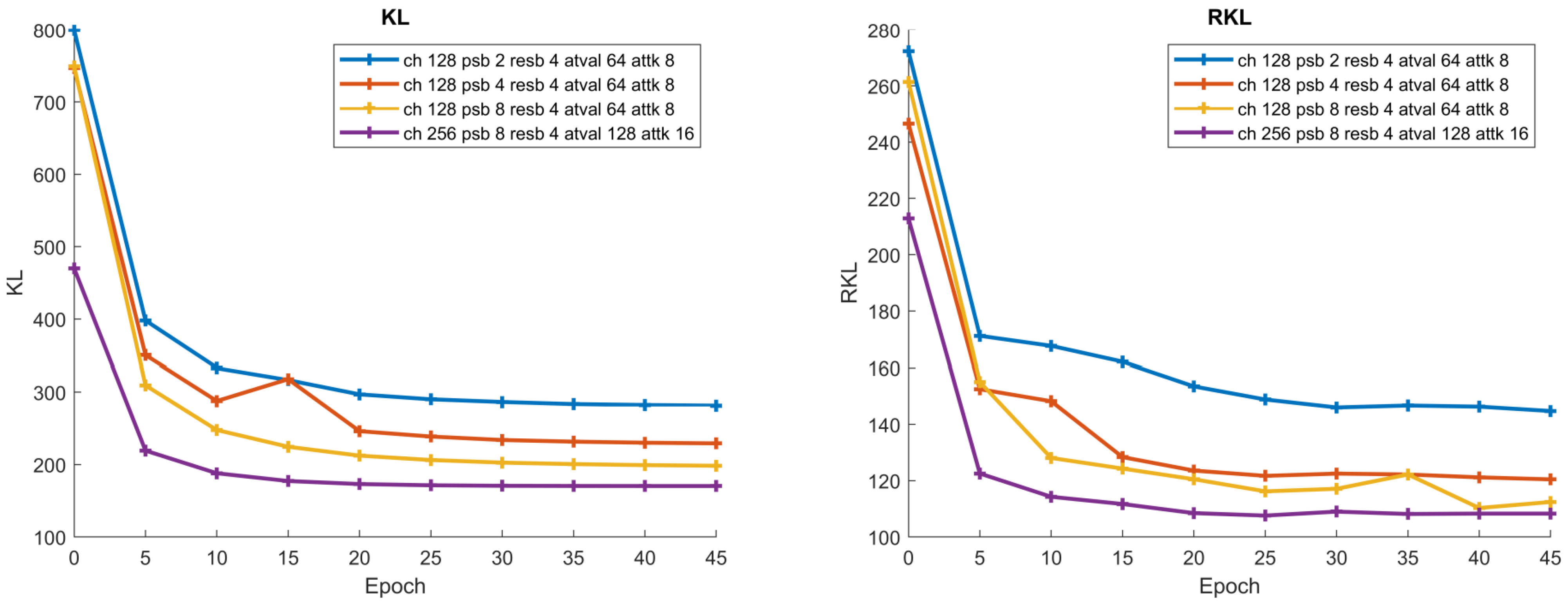
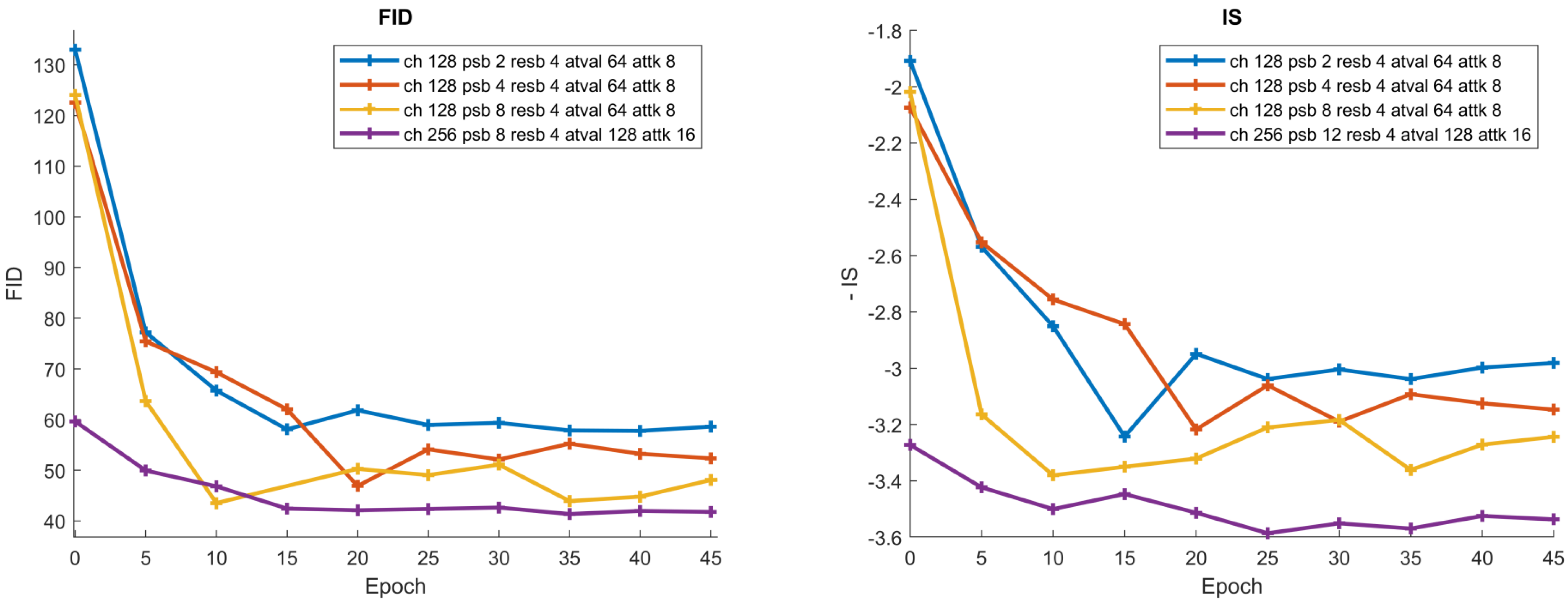
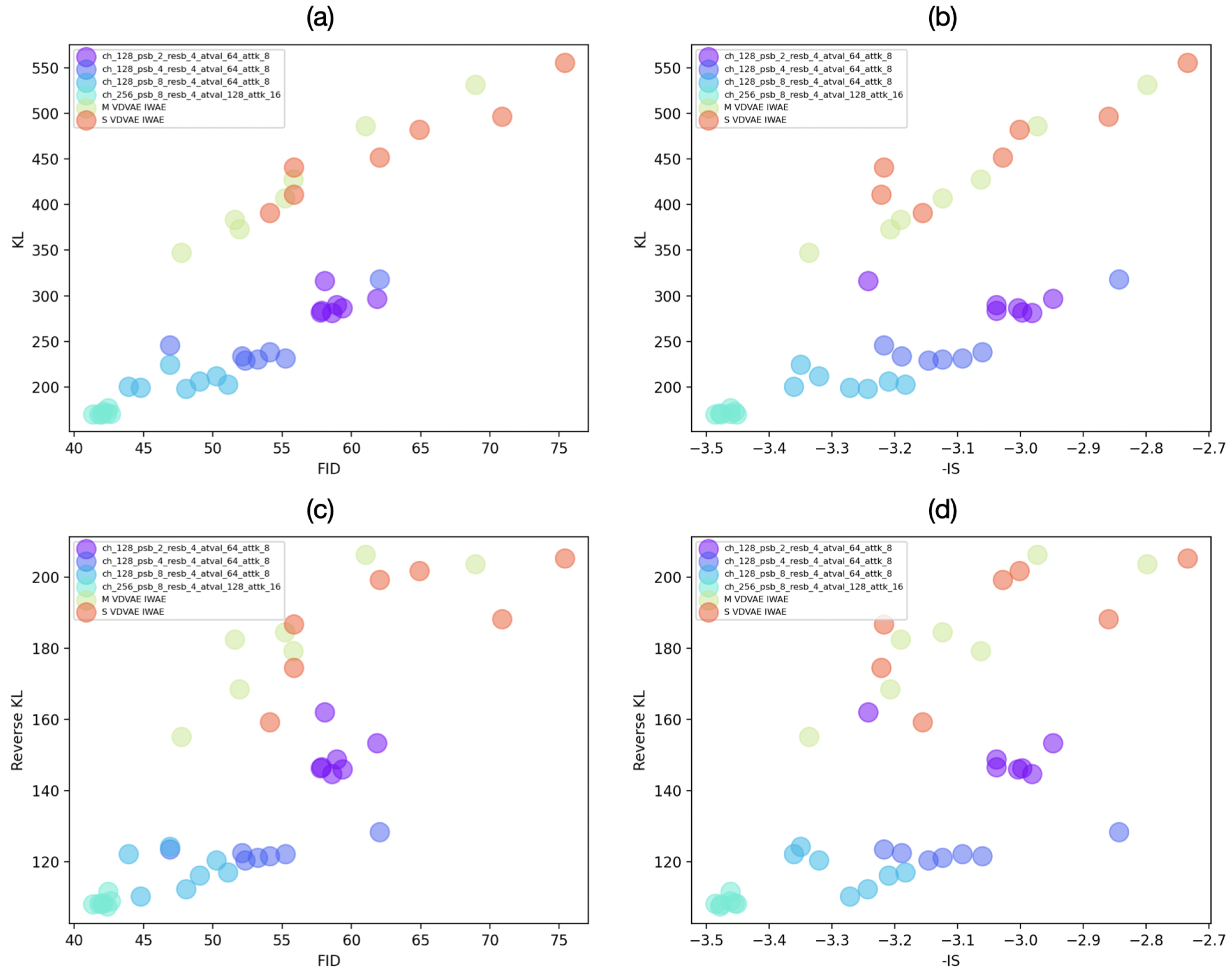
We first train four PixelSnail variants on our NotImageNet32 dataset and plot the KL, RKL, FID, and IS (we plot the negative IS, so lower is better for all metrics) along with the training for test set in Figure 4 and Figure 5. It can easily be seen that after 15–20 epochs both KL and RKL change slowly, but the FID and IS are much more volatile. Each dot in the graph represents a score that has been measured on a different epoch on a different model. To assess the variance in the results we used the jackknife resampling method [34]. The error bars are small ( 10 3 scale in most cases), hence they are unnoticeable. One can see from this figure that as we increase the model capacity, the KL score improves. Model-generated samples are included in Appendix D. Interestingly, the KL and RKL have a high agreement, even if they penalize very different mistakes in the model. In stark contrast, we see that the FID, and especially IS, are much more volatile and can give very different scores to models that have very similar KL and RKL scores.
For another perspective, we plot in Figure 6 the FID and negative IS vs. KL and RKL. We observe a high correlation between FID/IS and KL and a weaker correlation between these metrics and the RKL. IS and FID also seem ill-suited for fine-grained comparisons between models. For high-quality models, e.g., light-blue dots in Figure 6, one can obtain a significant change in FID/IS without a significant change to KL/RKL. This can be very problematic, as when comparing similar models, e.g., testing various design choices, these metrics can imply significant improvement even when it is not seen in our probabilistic metrics. We add zoomed-in versions of this plot to Appendix A for greater clarity.

4.2. Ranking Correlation

To better quantitatively assess our previous observations, we compare how the metrics differ in their ranking of the various trained models. This is of great importance, as comparing different models is the primary goal of these metrics. To compare the ranking we compute Kendall’s τ ranking correlation (Table 1). We perform the correlation analysis for models that were trained for 15–45 epochs and ignore the first iterations of the training procedure. This is to focus more on the fine-grained comparisons.
The highest score in both ranking correlation methods is between KL and reverse KL with 0.889 Kendall’s τ (in bold). This may be surprising since these two methods measure different characteristics of the data. Confirming our previous observation, the FID and IS ranking scores are low, with FID outperforming IS. However, the extensions of FID do achieve better scores.
Another observation is the relatively low correlation between many of the different rankings. All of the inception ranking correlations, except one (KID and clean FID), indicate that one can obtain significantly different rankings by using a different metric.
Among the inception-based metrics, FID has the highest correlation with KL and RKL, which indicates that it is a more reliable metric than the others. IS/IS has the lowest ranking correlation of all the other models.

5. Discussion

This study contributes to the evolving field of generative model evaluation by introducing a novel evaluation protocol that utilizes a high-quality synthetic dataset, NotImageNet32, to compare probabilistic f-divergences like KL and RKL with empirical metrics such as FID and IS. Our findings indicate that while empirical metrics like FID and IS are widely used and correlate with some aspects of model performance, they exhibit considerable volatility and do not always align with changes observed in f-divergence metrics. This discrepancy underscores the complexities and potential limitations of using single metrics for model evaluation.

5.1. Comparison with Existing Literature

Our results align with previous studies that have critiqued the reliability of popular metrics like IS and FID, particularly in terms of their consistency and ability to generalize across different datasets and model types. For instance, the use of inception features has been shown to perform variably across non-ImageNet benchmarks, suggesting a need for more versatile and robust evaluation tools. Our study extends this narrative by demonstrating similar volatility and recommending the adoption of newer metrics like FID and the exploration of multiple metrics to provide a more comprehensive evaluation.

5.2. Implications of Findings

The observed volatility in empirical metrics, especially in high-stakes areas like generative model deployment in medical imaging or autonomous driving, could lead to misguided conclusions about model performance. By advocating for a combination of metrics and the introduction of a synthetic dataset as a standardized test-bed, our study proposes a pathway towards more reliable and interpretable evaluations. This approach could help mitigate risks associated with deploying under-evaluated or overestimated models in critical applications.

5.3. Limitations

The primary limitation of this study is its reliance on a single synthetic dataset, NotImageNet32, which, while providing a controlled environment for model evaluation, may not capture the diversity and complexity of real-world data. Additionally, our conclusions are based on the performance of likelihood-based generative models, which may not directly translate to implicit models such as GANs and diffusion models.

5.4. Future Research Directions

Future studies should aim to replicate and expand upon our findings by incorporating multiple synthetic and real-world datasets to assess the generalizability of the proposed metrics. Further research should also explore the development and validation of new metrics that can capture a broader range of model behaviors and better reflect real-world performance. Additionally, exploring the integration of human perceptual studies could provide a complementary perspective to purely computational metrics, offering a holistic view of model effectiveness.

6. Conclusions

We generated a high-quality synthetic dataset and compared standard empirical metrics, such as FID and IS, with probabilistic f-divergences like KL and RKL. Our analysis shows that although the empirical metrics generally correlate well and capture important trends, they demonstrate considerable volatility. Not all observed improvements in these metrics correspond to similar gains in KL- or RKL-divergences. Additionally, the inception score and its IS extensions tended to perform less effectively compared to other metrics.
Given the outcomes of our study and acknowledging that our analysis is based on a single synthetic dataset, we suggest the following cautious approaches for future research and application:
  • Consider phasing out the inception score, favoring FID for its reduced volatility.
  • Employ a combination of metrics (such as FID, KID, and clean FID) to help manage metric volatility and provide a more robust evaluation.
  • Explore using NotImageNet32 as a potential test-bed for likelihood-based generative models to further assess its efficacy across various generative modeling scenarios.

Author Contributions

E.B. was actively involved in the hands-on execution and collaborated closely with E.F., who guided and refined E.B.’s ideas, ensuring the project’s alignment with theoretical and practical applications. C.P. provided significant contributions in coding and implementation. All authors have read and agreed to the published version of the manuscript.

Funding

This project has received funding by the Israeli Council for Higher Education, Data Science Program (“Audience” project).

Data Availability Statement

https://github.com/eyalbetzalel/notimagenet32, accessed on 25 May 2024 (NotImageNet32 dataset).

Conflicts of Interest

The authors declare no conflicts of interest.

Appendix A. Volatility Analysis of High-Quality Models

In Figure A1, one can see that the FID score dramatically changes although there is not much change in the KL or in the RKL metrics. This may indicate the volatility of this method.
Figure A1. Evaluation metrics through the training of four PixelSnail and two VD-VAE models of varying sizes. Zoom-in on high-quality models.
Make 06 00073 g0a1

Appendix B. Technical Details on Experiment’s Generative Models’ Architecture

As mentioned in Section 4, we create different models by setting different hyper-parameters in order to compare performances between them. In order to enable accurate reproduction capability, we describe the set of parameters we used.

Appendix B.1. PixelSnail

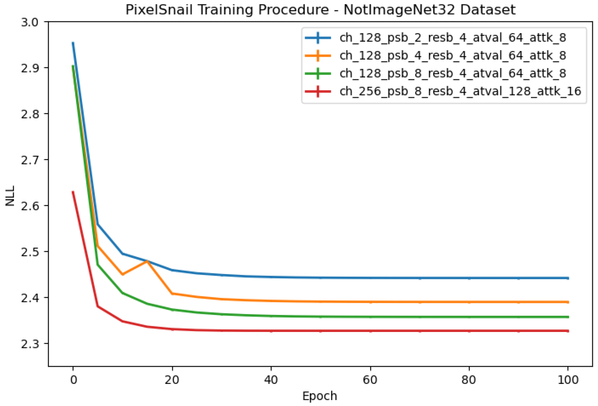
The PixelSnail architecture is primarily composed of two main components: a residual block, which applies several 2D-convolutions to its input, each with residual connections; and the attention block, which performs a single key–value lookup. It projects the input to a lower dimensionality to produce the keys and values and then uses softmax attention. The model is built from several PixelSnail blocks concatenated to one another, each interleaving the residual blocks and attention blocks mentioned earlier. We used Adam optimizer with LR 0.0001 and multiplicative LR scheduler with lambada LR 0.999977. The loss function changed to the mean cross-entropy over 512 discrete clusters. All the other parameters that make up the model are described in Table A1.
Table A1. PixelSnail hyper-parameters.
SizeChannelsPixelSnail BlocksResidual BlocksAttention ValuesAttention Keys
S12824648
M12844648
L12884648
XL2568412816
Figure A2. NLL score on the training set for different PixelSnail models on NotImageNet32.
Make 06 00073 g0a2

Appendix B.2. VD-VAE

The VD-VAE network is built from an encoder and decoder. In the encoder, there are regular blocks, which receive an input and output an output with the same dimension, and down-rate blocks that receive input and output an output with a lower dimension. The difference between these two blocks is an avg_pool2d at the end of the down-rate block. In the decoder, there are regular blocks and mixin blocks. The regular blocks receive an input and output an output with the same dimension. The input is fed from the previous layer and the parallel layer in the encoder. The mixin block performs interpolation to a higher dimension.
Table A2. VD-VAE hyper-parameters.
SizeEncoderDecoder
S32 × 5, 32d2, 16 × 4, 16d2, 8 × 4, 8d2, 4 × 4, 4d4, 1 × 21 × 2, 4m1, 4 × 4, 8m4, 8 × 3, 16m8, 16 × 8, 32m16, 32 × 20
M32 × 10, 32d2, 16 × 5, 16d2, 8 × 8, 8d2, 4 × 6, 4d4, 1 × 41 × 2, 4m1, 4 × 4, 8m4, 8 × 8, 16m8, 16 × 10, 32m16, 32 × 30
In Table A2, × means how many regular blocks are concatenated in a row. For example, 32 × 10 means 10 blocks in a row with a 32-channel input. d means a down-rate block. The following number is the factor of the pooling. m means an unpool (mixin) block, for example, 32m16 means 32 is the output dimensionality with 16 layers in the mixin block.
Other hyper-parameters that were changed include the EMA rate, to 0.999, warm-up iterations, to 1, learning rate, to 0.00005, grad clip, to 200, and skip threshold, to 300. We used the Adam optimizer with β 1 = 0.9 and β 2 = 0.9 . Other hyper-parameters were configured as mentioned in the VD-VAE article.

Appendix C. Supplementary Model Correlation Measurements

In Table A3, one can see that the Pearson correlation is high for most of the evaluated methods. This is consistent with the conclusion presented in the article on the ability of the current evaluation methods to capture trends.
Table A3. Pearson’s ρ correlation.
KLRKLFIDISISKIDFIDClean FID
KL10.9760.82170.70880.56560.90110.9110.8962
RKL0.97610.78390.65590.52790.85520.85850.8493
FID0.82170.783910.94410.90530.97710.95830.9829
IS0.70880.65590.944110.96570.90470.88580.9139
IS0.56560.52790.90530.965710.83010.7990.8407
KID0.90110.85520.97710.90470.830110.98250.998
FID0.9110.85850.95830.88580.7990.982510.9863
Clean FID0.89620.84930.98290.91390.84070.9980.98631
In Table A4, we present the Spearman’s ranking correlation, another ranking correlation method that is similar to Kendall’s τ and presents similar results.
Table A4. Spearman’s ρ ranking correlation.
KLRKLFIDISISKIDFIDClean FID
KL10.97790.84490.73940.60640.92010.93530.9242
RKL0.977910.81180.69210.56930.88280.88830.8865
FID0.84490.811810.92380.89340.95870.91650.9627
IS0.73940.69210.923810.95480.89040.8470.8799
IS0.60640.56930.89340.954810.7990.74220.7922
KID0.92010.88280.95870.89040.79910.96560.9964
FID0.93530.88830.91650.8470.74220.965610.9715
Clean FID0.92420.88650.96270.87990.79220.99640.97151

Appendix D. Sample Examples

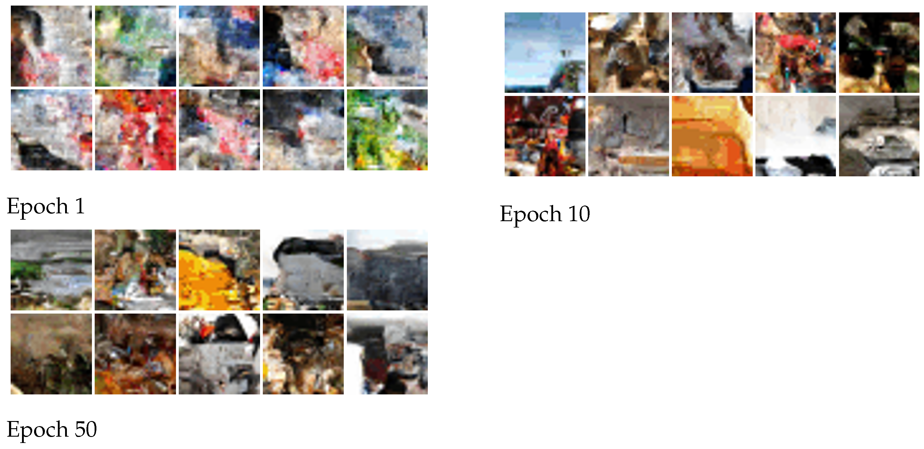
These samples were generated from the different models under test in Section 4, each subfigure was generated on a different epoch while training the models on the NotImageNet32 dataset. Figure A3 and Figure A4 are samples from the large PixelSnail model and the medium VD-VAE model, respectively. More details on the models are given in Appendix B.
Figure A3. PixelSnail model samples.
Make 06 00073 g0a3
Figure A4. VD-VAE model samples.
Make 06 00073 g0a4

References

  1. Goodfellow, I.J.; Pouget-Abadie, J.; Mirza, M.; Xu, B.; Warde-Farley, D.; Ozair, S.; Courville, A.C.; Bengio, Y. Generative Adversarial Nets. In Proceedings of the Neural Information Processing Systems (NeurIPS), Montreal, QC, Canada, 8–13 December 2014. [Google Scholar]
  2. Karras, T.; Laine, S.; Aittala, M.; Hellsten, J.; Lehtinen, J.; Aila, T. Analyzing and Improving the Image Quality of StyleGAN. In Proceedings of the Conference on Computer Vision and Pattern Recognition, CVPR, Virtually, 14–19 June 2020. [Google Scholar]
  3. Ramesh, A.; Dhariwal, P.; Nichol, A.; Chu, C.; Chen, M. Hierarchical Text-Conditional Image Generation with CLIP Latents. arXiv 2022, arXiv:2204.06125. [Google Scholar]
  4. Kong, J.; Kim, J.; Bae, J. HiFi-GAN: Generative Adversarial Networks for Efficient and High Fidelity Speech Synthesis. In Proceedings of the Advances in Neural Information Processing Systems (NeurIPS), Virtually, 6–12 December 2020. [Google Scholar]
  5. Ranaldi, L.; Pucci, G. Knowing Knowledge: Epistemological Study of Knowledge in Transformers. Appl. Sci. 2023, 13, 677. [Google Scholar] [CrossRef]
  6. Salimans, T.; Goodfellow, I.J.; Zaremba, W.; Cheung, V.; Radford, A.; Chen, X. Improved Techniques for Training GANs. In Proceedings of the Advances in Neural Information Processing Systems (NeurIPS), Barcelona, Spain, 5–10 December 2016. [Google Scholar]
  7. Heusel, M.; Ramsauer, H.; Unterthiner, T.; Nessler, B.; Hochreiter, S. GANs Trained by a Two Time-Scale Update Rule Converge to a Local Nash Equilibrium. arXiv 2018, arXiv:1706.08500. [Google Scholar]
  8. Deng, J.; Dong, W.; Socher, R.; Li, L.-J.; Li, K.; Li, F.F. ImageNet: A large-scale hierarchical image database. In Proceedings of the 2009 IEEE Conference on Computer Vision and Pattern Recognition, Miami, FL, USA, 20–25 June 2009; pp. 248–255. [Google Scholar] [CrossRef]
  9. Barratt, S.T.; Sharma, R. A Note on the Inception Score. arXiv 2018, arXiv:1801.01973. [Google Scholar]
  10. Parmar, G.; Zhang, R.; Zhu, J. On Buggy Resizing Libraries and Surprising Subtleties in FID Calculation. arXiv 2021, arXiv:2104.11222. [Google Scholar]
  11. Kingma, D.P.; Welling, M. Auto-Encoding Variational Bayes. arXiv 2013, arXiv:1312.6114. [Google Scholar]
  12. Chen, M.; Radford, A.; Child, R.; Wu, J.; Jun, H.; Luan, D.; Sutskever, I. Generative Pretraining From Pixels. In Proceedings of the International Conference on Machine Learning, (ICML), Virtual, 13–18 July 2020. [Google Scholar]
  13. Arjovsky, M.; Chintala, S.; Bottou, L. Wasserstein GAN. arXiv 2017, arXiv:1701.07875. [Google Scholar] [CrossRef]
  14. Bińkowski, M.; Sutherland, D.J.; Arbel, M.; Gretton, A. Demystifying mmd gans. arXiv 2018, arXiv:1801.01401. [Google Scholar]
  15. Chong, M.J.; Forsyth, D. Effectively unbiased fid and inception score and where to find them. In Proceedings of the Proceedings of the IEEE/CVF Conference on Computer Vision and Pattern Recognition, Seattle, WA, USA, 13–19 June 2020; pp. 6070–6079. [Google Scholar]
  16. Parmar, G.; Zhang, R.; Zhu, J.Y. On Aliased Resizing and Surprising Subtleties in GAN Evaluation. In Proceedings of the 2022 IEEE/CVF Conference on Computer Vision and Pattern Recognition (CVPR), New Orleans, LA, USA, 18–24 June 2022. [Google Scholar]
  17. KENDALL, M.G. A new measure of rank correlation. Biometrika 1938, 30, 81–93. [Google Scholar] [CrossRef]
  18. Bond-Taylor, S.; Leach, A.; Long, Y.; Willcocks, C.G. Deep Generative Modelling: A Comparative Review of VAEs, GANs, Normalizing Flows, Energy-Based and Autoregressive Models. IEEE Trans. Pattern Anal. Mach. Intell. 2021, 44, 7327–7347. [Google Scholar] [CrossRef] [PubMed]
  19. Borji, A. Pros and Cons of GAN Evaluation Measures: New Developments. arXiv 2021, arXiv:2103.09396. [Google Scholar] [CrossRef]
  20. Theis, L.; van den Oord, A.; Bethge, M. A note on the evaluation of generative models. In Proceedings of the 4th International Conference on Learning Representations, ICLR 2016, San Juan, PR, USA, 2–4 May 2016. [Google Scholar]
  21. Lee, J.; Lee, J.S. TREND: Truncated Generalized Normal Density Estimation of Inception Embeddings for Accurate GAN Evaluation. arXiv 2021, arXiv:2104.14767. [Google Scholar] [CrossRef]
  22. Xu, Q.; Huang, G.; Yuan, Y.; Guo, C.; Sun, Y.; Wu, F.; Weinberger, K. An empirical study on evaluation metrics of generative adversarial networks. arXiv 2018, arXiv:1806.07755. [Google Scholar] [CrossRef]
  23. Fedus, W.; Rosca, M.; Lakshminarayanan, B.; Dai, A.M.; Mohamed, S.; Goodfellow, I.J. Many Paths to Equilibrium: GANs Do Not Need to Decrease a Divergence At Every Step. arXiv 2018, arXiv:1710.08446. [Google Scholar]
  24. Lucic, M.; Kurach, K.; Michalski, M.; Gelly, S.; Bousquet, O. Are GANs Created Equal? A Large-Scale Study. In Proceedings of the Advances in Neural Information Processing Systems 31: Annual Conference on Neural Information Processing Systems 2018, NeurIPS 2018, Montréal, QC, Canada, 3–8 December 2018. [Google Scholar]
  25. Shmelkov, K.; Schmid, C.; Alahari, K. How Good Is My GAN? In Proceedings of the Computer Vision-ECCV 2018-15th European Conference, Munich, Germany, 8–14 September 2018.
  26. Lesort, T.; Stoian, A.; Goudou, J.; Filliat, D. Training Discriminative Models to Evaluate Generative Ones. In Proceedings of the Artificial Neural Networks and Machine Learning-ICANN 2019: Image Processing-28th International Conference on Artificial Neural Networks, Munich, Germany, 17–19 September 2019. [Google Scholar]
  27. Santurkar, S.; Schmidt, L.; Madry, A. A Classification-Based Study of Covariate Shift in GAN Distributions. In Proceedings of the Proceedings of the 35th International Conference on Machine Learning, ICML 2018, Stockholm, Sweden, 10–15 July 2018. [Google Scholar]
  28. Ravuri, S.V.; Vinyals, O. Classification Accuracy Score for Conditional Generative Models. In Proceedings of the Advances in Neural Information Processing Systems 32: Annual Conference on Neural Information Processing Systems 2019, NeurIPS 2019, Vancouver, BC, Canada, 8–14 December 2019. [Google Scholar]
  29. Sajjadi, M.S.M.; Bachem, O.; Lucic, M.; Bousquet, O.; Gelly, S. Assessing Generative Models via Precision and Recall. arXiv 2018, arXiv:1806.00035. [Google Scholar] [CrossRef]
  30. Kynkäänniemi, T.; Karras, T.; Laine, S.; Lehtinen, J.; Aila, T. Improved Precision and Recall Metric for Assessing Generative Models. arXiv 2019, arXiv:1904.06991. [Google Scholar] [CrossRef]
  31. Chen, X.; Mishra, N.; Rohaninejad, M.; Abbeel, P. PixelSNAIL: An Improved Autoregressive Generative Model. arXiv 2017, arXiv:1712.09763. [Google Scholar]
  32. Child, R. Very Deep VAEs Generalize Autoregressive Models and Can Outperform Them on Images. arXiv 2021, arXiv:2011.10650. [Google Scholar]
  33. Burda, Y.; Grosse, R.; Salakhutdinov, R. Importance Weighted Autoencoders. arXiv 2016, arXiv:1509.00519. [Google Scholar]
  34. Tukey, J. Bias and confidence in not quite large samples. Ann. Math. Statist. 1958, 29, 614. [Google Scholar]
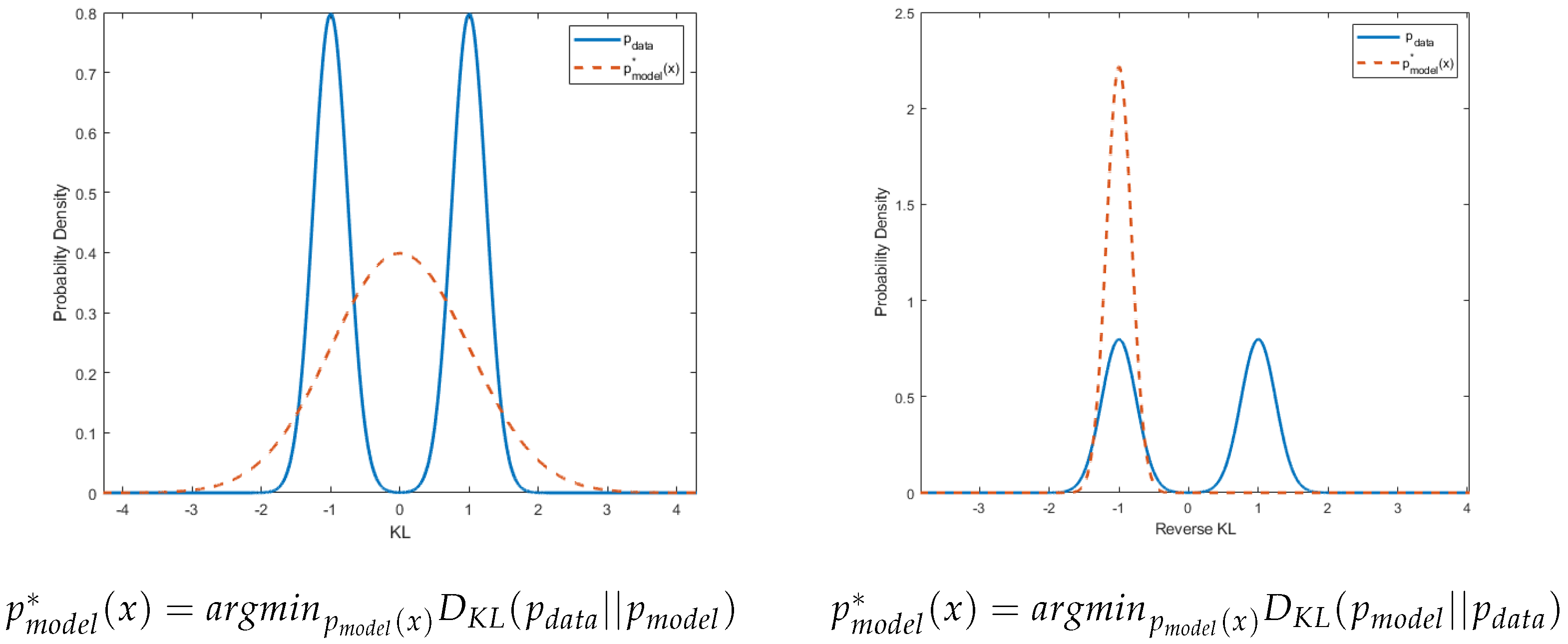
Figure 1. Optimizing p m o d e l with KL criteria pushes the model to cover all aspects of p d a t a , hence it is more exclusive, while optimizing it with reverse KL criteria encourages the model to cover the area with the largest probability, hence it is more inclusive.
Make 06 00073 g001
Figure 2. Illustration: X are ImageNet images; X ^ are synthetic images sampled from image-GPT; p d a t a ( X ^ ) is ground truth likelihood from image-GPT for synthetic images; and p m o d e l ( X ^ ) is likelihood estimation of p d a t a ( X ^ ) , calculated by the evaluated model, in this case, PixelSnail.
Make 06 00073 g002
Figure 3. Examples of photos that are generated by image-GPT. Each photo’s explicit likelihood can be measured.
Make 06 00073 g003
Figure 4. Test of KL and RKL of PixelSnail models through training.
Make 06 00073 g004
Figure 5. Test of FID and negative IS of PixelSnail models through training. We plot the negative inception score, so lower is better for all metrics. Details on the hyper-parameters summarized in the legend are in the Appendix B.
Make 06 00073 g005
Figure 6. Evaluation metrics through the training of four PixelSnail and two VD-VAE models of varying sizes. (a) FID vs. KL, (b) -IS vs. KL, (c) FID vs. RKL, (d) -IS vs. RKL. We plot the negative inception score, so lower is better for all metrics.
Make 06 00073 g006
Table 1. Kendall’s τ correlation between different metrics. A correlation score indicates the degree of agreement between two scoring methods.
KLRKLFIDISISKIDFIDClean FID
KL10.88950.70270.58890.46810.77700.80950.7909
RKL0.889510.63370.52440.43140.71050.72670.7198
FID0.70270.633710.79790.71890.85130.80020.8699
IS0.58890.52440.797910.82810.73290.68180.7236
IS0.46810.43140.71890.828110.61670.57490.6074
KID0.77700.71050.85130.73290.616710.86060.9675
FID0.80950.72670.80020.68180.57490.860610.8746
Clean FID0.79090.71980.86990.72360.60740.96750.87461
Disclaimer/Publisher’s Note: The statements, opinions and data contained in all publications are solely those of the individual author(s) and contributor(s) and not of MDPI and/or the editor(s). MDPI and/or the editor(s) disclaim responsibility for any injury to people or property resulting from any ideas, methods, instructions or products referred to in the content.