Interaction Difference Hypothesis Test for Prediction Models

Abstract

Machine learning research focuses on the improvement of prediction performance. Progress was made with black-box models that flexibly adapt to the given data. However, due to their increased complexity, black-box models are more difficult to interpret. To address this issue, techniques for interpretable machine learning have been developed, yet there is still a lack of methods to reliably identify interaction effects between predictors under uncertainty. In this work, we present a model-agnostic hypothesis test for the identification of interaction effects in black-box machine learning models. The test statistic is based on the difference between the variance of the estimated prediction function and a version of the estimated prediction function without interaction effects derived via partial dependence functions. The properties of the proposed hypothesis test were explored in simulations of linear and nonlinear models. The proposed hypothesis test can be applied to any black-box prediction model, and the null hypothesis of the test can be flexibly specified according to the research question of interest. Furthermore, the test is computationally fast to apply, as the null distribution does not require the resampling or refitting of black-box prediction models.

1. Background

In the context of machine learning, one of the main goals is to estimate and tune prediction models in order to optimize predefined performance criteria [1]. In the ongoing academic debate, [2] argued that the attribution of causal factors may require a larger sample size than estimating a prediction model. This is in line with [3], who showed that causality can be linked with prediction robustness. The research area of interpretable machine learning (IML) tries to bridge the gap between prediction and classical statistical inference by making complex black-box predictions more understandable [4]. A black-box model is characterized by an input–output relationship between covariates and a response [5]. In this approach, the internal structure of the box is not explicitly modeled and is regarded as unknown. The Rashomon effect [6] originates from a Japanese movie from 1950. The main plot is about a crime happening in the 12th century, which is shown from the perspectives of multiple people. Differences in those experiences show that it is hard to uncover later what really happened because, for a given set of facts, there are a multitude of compatible stories. Analogously, in machine learning, there are many different models that explain the observed data equally well. The problem of empirical induction has a long history in the philosophy of science. For example, the skepticism of David Hume, dating back to the 18th century [7], or Duhem’s theses stated that the falsifiability of a single hypothesis is inconclusive [8]. This work will not address this philosophical problem, but it takes instead a pragmatic approach [9]. It is assumed that the primary goal is to optimize prediction performance [10] in a given context. There is some evidence of a trade-off between prediction performance and interpretability in the literature [11,12,13,14]. However, prediction can benefit from interpretability as well because a deeper qualitative understanding of why a model produces a given output and not another can help generate more robust out-of-sample predictions. Therefore, it is recommended to use interpretability approaches that do not harm prediction performance but help incorporate human considerations into explainable artificial intelligence [15].

IML allows a researcher to benefit from advances in machine learning research and still explore the properties of the model afterwards to increase the interpretability of the model. Example applications include designing regulatorily compliant, fair [16], transparent, and trustworthy prediction models [17]. Another area of IML focuses on the interpretation of the effects of covariates on prediction [18,19,20]. Here, the focus is on global model interpretability, which means that the prediction function over the whole covariate distribution is the focus of interest instead of explaining single local predictions for specific covariate values [21].

The following sections, Section 1.1, Section 1.2 and Section 1.3, introduce the background knowledge required to understand the new proposed interaction difference hypothesis test for prediction models that is defined in Section 2. Firstly, a measure of how a prediction function changes, on average, for different values of a given set of covariates is introduced in Section 1.1. This measure is an essential component used in the definition of interaction effects. Secondly, Section 1.2 describes a general definition of interaction effects for black-box models, which is based on an additive decomposition of the predictions. The decomposition is illustrated using a linear regression example. Thirdly, Section 1.3 provides an overview of existing approaches to quantify interaction effects. Finally, the last introductory section, Section 1.4, describes the null hypothesis of the interaction test and the disadvantages of the previously described, existing approaches that will be addressed in this work.

1.1. Partial Dependence Functions

A global summary of the impact of one covariate on the predictions is the partial dependence (PD) plot [22]. Let $\mathit{X}$$\in {\mathbb{R}}^{n\times p}$ be the observed matrix of p covariates with n independent observations of the multivariate random vector $\mathit{x}$$\in {\mathbb{R}}^p$ and $\widehat{f}\left(\mathit{x}\right)$ be the estimated predictions of a statistical model of the prediction function $f\left(\mathit{x}\right)$ on the population level. $f\left(\mathit{x}\right)$ does not necessarily equal the covariate–response relationship in the data-generating process. It is assumed that $\widehat{f}\left(\mathit{x}\right)$ was estimated, as well as tuned, prior to IML analysis with respect to prediction performance with the test data. Define $S=\left\{1,\dots ,p\right\}$ to be the set of all indices of covariates, and the set $s\subset S$ corresponds to indices of chosen covariates of interest. The term ${\mathrm{E}}_{{\mathit{x}}_{S\setminus s}}\left({\mathit{x}}_s\right)$ is defined as the expectation over the marginal (joint) distribution of all variables not in set s (denoted as ${\mathit{x}}_{S\setminus s}$) for fixed values ${\mathit{x}}_s$ of the variables in set s (for a comparison, see [22] Section 8.1). Note that multiple column indices are denoted using set brackets in the subscript; for example, $s=\left\{1,2\right\}$ yields ${\mathit{x}}_{\left\{1,2\right\}}$, and empty subscripts describe all available indices (for example, the second column with all observations, ${\mathit{X}}_{,2}$). The PD function is given via

$$\begin{array}{cc}\hfill & \mathrm{PD}\left({\mathit{x}}_s\right)={\mathrm{E}}_{{\mathit{x}}_{S\setminus s}}\left(f\left({\mathit{x}}_s,{\mathit{x}}_{S\setminus s}\right)\right)\mathrm{and}\mathrm{estimated}\mathrm{by}\hfill \end{array}$$

(1)

$$\begin{array}{cc}\hfill & \widehat{\mathrm{PD}}\left({\mathit{x}}_s\right)=\frac{1}{n}\sum _{i=1}^n\widehat{f}\left({\mathit{x}}_s,{\mathit{X}}_{i,S\setminus s}\right).\hfill \end{array}$$

(2)

For example, in the case of $p=5,s=\left\{1,2,3\right\}$, the function $\mathrm{PD}\left({\mathit{x}}_{\left\{1,2,3\right\}}\right)$ is the expected value of the predictions with respect to the covariate distribution ${\mathit{x}}_{\left\{4,5\right\}}$, given the observed covariate values ${\mathit{X}}_{,\left\{1,2,3\right\}}$. If $s=\varnothing$; then, $\mathrm{PD}\left({\mathit{x}}_{\varnothing }\right)$ corresponds to the expected marginal prediction over all covariates, ${\mathit{x}}_{\left\{1,2,3,4,5\right\}}$. Note that, in the case of $s=S$, the PD function equals the original model predictions, $\mathrm{PD}\left({\mathit{x}}_s\right)=f\left(\mathit{x}\right)$, and the function argument ${\mathit{x}}_s$ values do not necessarily need to correspond to training data.

1.2. Interactions in Black-Box Models

First, we briefly recap what interaction effects are in a linear model context [23]. Consider the simple case of a linear model prediction function with two independent covariates, ${\mathit{x}}_1,{\mathit{x}}_2$, main and interaction effects:

$$\begin{array}{cc}\hfill & f\left(\mathit{x}\right)={\beta }_0+{\mathit{x}}_1{\beta }_1+{\mathit{x}}_2{\beta }_2+{\mathit{x}}_1{\mathit{x}}_2{\beta }_{1,2}.\hfill \end{array}$$

(3)

The main effects, ${\beta }_1$ and ${\beta }_2$, represent how the prediction function changes linearly, given ${\beta }_{1,2}=0$, if the covariate of interest is increased by one unit. In contrast, the interaction effect ${\beta }_{1,2}\ne 0$ of covariates ${\mathit{x}}_1$ and ${\mathit{x}}_2$ contributes additional flexibility that goes beyond the main effects and the global intercept ${\beta }_0$. Let the difference term be $d_{\mathrm{linear}}=f\left(\mathit{x}\right)-{\mathit{x}}_1{\beta }_1-{\mathit{x}}_2{\beta }_2-{\beta }_0={\mathit{x}}_1{\mathit{x}}_2{\beta }_{1,2}$. If the interaction effect is ${\beta }_{1,2}\ne 0$, then the variance of the difference term ${\mathrm{Var}}_{\mathit{x}}\left(d_{\mathrm{linear}}\right)$ is greater than zero. Similarly, if ${\beta }_1\ne 0$, then ${\mathrm{Var}}_{\mathit{x}}\left({\mathit{x}}_1{\beta }_1\right)>0$ follows.

One advantage of black-box models (for example, neural networks) is their capacity to fit higher-order interaction effects in a data-driven way without the need to explicitly prespecify them. Knowledge of the presence of such interaction effects would increase the scientific understanding of a given phenomenon, and the absence of interaction effects could be used to simplify black-box prediction models with little degradation in performance. In this context, interaction effects can be defined within the functional ANOVA decomposition framework [24]. The prediction function $f\left(\mathit{x}\right)$ is decomposed into a sum of additive orthogonal terms, $\tilde{f}\left({\mathit{x}}_{\tilde{s}}\right)$, of sets $\tilde{s}$. Each term recursively subtracts all respective previously derived lower-order terms within set $\tilde{s}$. In this work, we use PD functions to define the functional ANOVA terms $\tilde{f}\left({\mathit{x}}_{\tilde{s}}\right)$. In the simple linear regression example in Equation (3), the first ANOVA term would correspond to the expected value of the prediction

$$\begin{array}{cc}\hfill & \tilde{f}\left({\mathit{x}}_{\varnothing }\right)=\mathrm{PD}\left({\mathit{x}}_{\varnothing }\right)\hfill \end{array}$$

(4)

$$\begin{array}{cc}\hfill & ={\beta }_0+{\mu }_1{\beta }_1+{\mu }_2{\beta }_2+{\mu }_{1,2}{\beta }_{1,2}\hfill \end{array}$$

(5)

with ${\mu }_j$ being the expected value of the covariates or, in the case of ${\mu }_{1,2}$, the expected value of the product of the covariates. By definition, the functional ANOVA main effects, $\tilde{f}\left({\mathit{x}}_1\right),\tilde{f}\left({\mathit{x}}_2\right)$, consist of the PD functions of ${\mathit{x}}_1,{\mathit{x}}_2$, minus the sum of all possible respective lower-order effects. In the case of one covariate, only the empty set needs to be subtracted:

$$\begin{array}{cc}\hfill & \tilde{f}\left({\mathit{x}}_1\right)=\mathrm{PD}\left({\mathit{x}}_1\right)-\tilde{f}\left({\mathit{x}}_{\varnothing }\right)\mathrm{and}\hfill \end{array}$$

(6)

$$\begin{array}{cc}\hfill & \tilde{f}\left({\mathit{x}}_2\right)=\mathrm{PD}\left({\mathit{x}}_2\right)-\tilde{f}\left({\mathit{x}}_{\varnothing }\right).\hfill \end{array}$$

(7)

In the concrete scenario, the functional ANOVA main effects are given by

$$\begin{array}{cc}\hfill & \mathrm{PD}\left({\mathit{x}}_1\right)={\beta }_0+{\mathit{x}}_1{\beta }_1+{\mu }_2{\beta }_2+{\mathit{x}}_1{\mu }_2{\beta }_{1,2}\hfill \end{array}$$

(8)

$$\begin{array}{cc}\hfill & \Rightarrow \tilde{f}\left({\mathit{x}}_1\right)={\mathit{x}}_1\left({\beta }_1+{\mu }_2{\beta }_{1,2}\right)-{\mu }_1{\beta }_1-{\mu }_{1,2}{\beta }_{1,2}\mathrm{and}\hfill \end{array}$$

(9)

$$\begin{array}{cc}\hfill & \mathrm{PD}\left({\mathit{x}}_2\right)={\beta }_0+{\mu }_1{\beta }_1+{\mathit{x}}_2{\beta }_2+{\mu }_1{\mathit{x}}_2{\beta }_{1,2}\hfill \end{array}$$

(10)

$$\begin{array}{cc}\hfill & \Rightarrow \tilde{f}\left({\mathit{x}}_2\right)={\mathit{x}}_2\left({\beta }_2+{\mu }_1{\beta }_{1,2}\right)-{\mu }_2{\beta }_2-{\mu }_{1,2}{\beta }_{1,2}.\hfill \end{array}$$

(11)

If ${\beta }_{1,2}=0$, then $\tilde{f}\left({\mathit{x}}_1\right)$ and $\tilde{f}\left({\mathit{x}}_2\right)$ correspond analogously to centered main effects in the linear model. In the case of the second-order functional ANOVA term $\tilde{f}\left({\mathit{x}}_{\left\{1,2\right\}}\right)$, two first-order terms that are contained in set $\left\{1,2\right\}$ need to be substracted, as well as the empty set, to ensure the orthogonality of second- and first-order ANOVA terms. The second-order interaction effect in terms of the functional ANOVA is, then,

$$\begin{array}{cc}\hfill & \tilde{f}\left({\mathit{x}}_{\left\{1,2\right\}}\right)=\mathrm{PD}\left({\mathit{x}}_{\left\{1,2\right\}}\right)-\tilde{f}\left({\mathit{x}}_1\right)-\tilde{f}\left({\mathit{x}}_2\right)-\tilde{f}\left({\mathit{x}}_{\varnothing }\right),\hfill \end{array}$$

(12)

$$\begin{array}{cc}\hfill & \mathrm{PD}\left({\mathit{x}}_{\left\{1,2\right\}}\right)=f\left(\mathit{x}\right)\mathrm{and}\hfill \end{array}$$

(13)

$$\begin{array}{cc}\hfill & \Rightarrow \tilde{f}\left({\mathit{x}}_{\left\{1,2\right\}}\right)={\mathit{x}}_1{\mathit{x}}_2{\beta }_{1,2}-{\mu }_1{\beta }_{1,2}-{\mu }_2{\beta }_{1,2}+{\mu }_{1,2}{\beta }_{1,2}.\hfill \end{array}$$

(14)

If ${\beta }_{1,2}\ne 0$, then ${\mathrm{Var}}_{\mathit{x}}\left[\tilde{f}\left({\mathit{x}}_{\left\{1,2\right\}}\right)\right]>0$, similar to the linear model context. If ${\beta }_{1,2}=0$, the functional ANOVA main effects have the property ${\mathrm{Var}}_{\mathit{x}}\left[\tilde{f}\left({\mathit{x}}_{\left\{j\right\}}\right)\right]>0$ for $j=\left\{1,2\right\}$, which is also shared within the linear model. Note that, if ${\beta }_{1,2}\ne 0$, then the functional ANOVA main effects include part of the linear model interaction effect in term ${\mathit{x}}_j{\mu }_{\left\{1,2\right\}\setminus j}{\beta }_{1,2}:j\in \left\{1,2\right\}$. Therefore, we analogously define ${\mathrm{Var}}_{\mathit{x}}\left[\tilde{f}\left({\mathit{x}}_{s^{★}}\right)\right]>0:s^{★}\subset S\wedge \left|s^{★}\right|\ge 2$ as interaction effects of at least order $\left|s^{★}\right|$ of the covariates in set $s^{★}$ of black-box models.

One disadvantage of functional ANOVA is that those derived terms are estimators based on data, and this uncertainty has to be taken into account when conducting inference. A distribution of the functional ANOVA terms under the null hypothesis of no interaction is not available. A second disadvantage is that the complexity to compute the decomposition grows exponentially with the number of covariates to $2^p$ possible elements. Furthermore, this concept works best with independent covariates, which is unrealistic in practice. A generalized functional ANOVA [25] includes covariate dependencies but requires solving a system of equations that is even more computationally demanding than the functional ANOVA decomposition. This limits the practical application to lower-order interaction terms [18].

1.3. Interaction Measures Based on PD Functions

Based on the concept of PD functions, [22] derived the ${\mathrm{H}}^2$ statistic to analyze interaction effects. The ${\mathrm{H}}^2$ statistic measures the variance in the differences between a prediction function and its restricted form under a given null hypothesis normalized by the variance of the prediction function to detect specific interaction effects. Note that the concrete form of ${\mathrm{H}}^2$ depends on the null hypothesis. For example, to test whether covariates in set s interact with any other covariates of set S, the statistic ${\mathrm{H}}_s^2$ is defined as

$$\begin{array}{cc}\hfill & {\mathrm{H}}_s^2=\frac{{\mathrm{Var}}_{{\mathit{x}}_s}\left(f\left(\mathit{x}\right)-\mathrm{PD}\left({\mathit{x}}_{S\setminus s}\right)-{\sum }_{j\in s}\mathrm{PD}\left({\mathit{x}}_j\right)\right)}{{\mathrm{Var}}_{\mathit{x}}\left(\mathrm{PD}\left(\mathit{x}\right)\right)}\mathrm{and}\mathrm{estimated}\mathrm{by}\hfill \end{array}$$

(15)

$$\begin{array}{cc}\hfill & {\widehat{\mathrm{H}}}_s^2=\frac{{\sum }_{i=1}^n{\left[\widehat{f}\left({\mathit{X}}_{i,S}\right)-\widehat{\mathrm{PD}}\left({\mathit{X}}_{i,S\setminus s}\right)-{\sum }_{j\in s}\widehat{\mathrm{PD}}\left({\mathit{X}}_{i,j}\right)\right]}^2}{{\sum }_{i=1}^n{\left[\widehat{\mathrm{PD}}\left({\mathit{X}}_{i,S}\right)\right]}^2}\hfill \end{array}$$

(16)

assuming centered PD functions. Equation (15) is an extension of Equation (45) in [22] to multiple covariates. It was derived by repeatedly applying Equation (42) in [22] for each element of s. Note that the difference of Equation (15) to Equations (43) and (46) by [22] is the hypothesis that is being tested. In the latter case, the hypothesis is to test for the presence of the specific three-way interaction between covariates ${\mathit{x}}_j,{\mathit{x}}_k,{\mathit{x}}_l$ that allows any two-way interaction to be present in the prediction model. This work focuses on testing any interaction effects of covariates in the prediction model specified in set s. In Section 1.4, the hypothesis of this work is described in more detail.

The statistic (15) was developed in the context of rule ensembles, and the flexible specification of interaction effects can be evaluated. The derived hypothesis test is a parametric bootstrap approach that simulates artificial data sets with a prediction model restricted to the null hypothesis of no interaction effects (Section 8.3 in [22]). Rule ensembles can be restricted to not include interaction effects by limiting the tree depth to one, but it does not work for different types of prediction models. Furthermore, the approach is computationally expensive due to the need to refit prediction models to artificial data sets, and the accuracy of the simulated p-value depends on the number of bootstrap replicates. The computational costs rise further due to the tuning process of hyperparameters, which are usually based on resampling methods like k-fold cross-validation. For an overview of recent developments in the field of hyperparameter optimization, we refer to [26].

Another measure to quantify interactions was developed by [27] that quantifies interactions between two covariates, ${\mathit{x}}_j$ and ${\mathit{x}}_k$, by estimating the standard deviation of the PD function of the ${\mathit{x}}_j$ conditional on values of ${\mathit{x}}_k$. This approach is restricted to two-way interactions. Generalizing this to scale higher-order interaction effects than two would reduce the number of available samples for estimating the standard deviation, and the number of possible combinations of the conditional covariates would increase exponentially. Note that there are also graphical tools to assess interaction effects, for example, [28,29]; however, these can only be meaningfully applied to illustrate lower-dimensional covariate interaction effects than three, and they do not quantify their method uncertainty analytically. Thus, an uncertainty assessment of these methods requires the usage of computer-intensive resampling methods that are not feasible with a large number of covariates.

1.4. Scope of Research

This work explored an interaction hypothesis test in model-agnostic form, meaning that it can be used with any kind of prediction model. It was assumed that the prediction model has enough capacity to potentially estimate interaction effects. In particular, consider the following null hypothesis that there is no interaction effect in the population involving any variable in s:

$$\begin{array}{cc}\hfill & H_0:f\left(\mathit{x}\right)=\mathrm{PD}\left({\mathit{x}}_{S\setminus s}\right)+\sum _{j\in s}\mathrm{PD}\left({\mathit{x}}_j\right)\mathrm{and}\mathrm{respectively}\hfill \end{array}$$

(17)

$$\begin{array}{cc}\hfill & H_1:f\left(\mathit{x}\right)\ne \mathrm{PD}\left({\mathit{x}}_{S\setminus s}\right)+\sum _{j\in s}\mathrm{PD}\left({\mathit{x}}_j\right).\hfill \end{array}$$

(18)

The set s describes the covariates of interest. For example, if $s=\left\{1,3\right\}$ and $S=\left\{1,2,3\right\}$, then it tests whether there is any interaction involving the first and third covariates. In this special case, the statistical test includes second- and third-order interaction effects. In general, the number of elements, $\left|s\right|$, determines the highest order of interaction effects considered in the hypothesis test.

Generally, one could consider ${\mathrm{H}}_s^2$; however, using measure ${\mathrm{H}}_s^2$ as the basis for the interaction test would have some disadvantages in practice:

• Simulations of ${\mathrm{H}}_s^2$ show increased false positive rates [27,30].
• There is no asymptotic null distribution of the hypothesis test of [22] for the presence of interactions available in model-agnostic form.
• The ${\mathrm{H}}_s^2$ interaction test is based on Monte Carlo simulations to quantify uncertainty [31], which are computationally runtime-intensive.
• To the best of the authors’ knowledge, no systematic power simulation in hypothesis interaction tests based on ${\mathrm{H}}_s^2$ was conducted.

This work addresses all of these issues. Furthermore, none of the existing IML approaches provide error-rate control [32], and thus, no severe testing is possible. Ref. [33] developed a statistically sophisticated philosophy of science in which the problem of induction is reduced to the practice of severe testing. To believe in a hypothesis is not only a function of the method or data used but also concerns how well the method was critically tested to rule out potential flaws. This work is a first step towards embedding IML methods into this statistical testing framework.

As an alternative to ${\mathrm{H}}_s^2$, the interaction difference (IAD) and the corresponding hypothesis interaction test are introduced in Section 2. It is shown how the IAD can be transformed into a test statistic that can be embedded into a two-sided, one-sample Z-test. Then, in Section 3, the asymptotic distribution of the test statistic based on test data is derived. Simulations of the proposed method are given in Section 4, which include the distribution of the proposed test statistic (Section 4.1), type 1 error, and power in linear (Section 4.2) models. The advantage of those simulation scenarios is that interaction effects can be more easily incorporated than in more complex black-box models in the design. Section 4.3 covers simulations of ${\widehat{z}}_4$ based on a random forest model. This situation is more realistic than the previous sections because, in linear models, one would not need this interaction test in practice. However, it is harder to control interaction effects in nonlinear simulation designs. The data analysis example in Section 5 focuses on a variant of the test statistic that includes covariate information.

2. Hypothesis Test of Interactions in Prediction Models

The concept of the proposed statistical test is to compare variances in the estimated prediction model $\widehat{f}$ and the estimated prediction model without interactions represented by PD functions. That means both variances are derived from the same data and, hence, dependent. Here, we follow the framework of [34] for robust tests of scale in paired samples. Those tests convert the hypothesis to allow standard asymptotical tests to be used. An advantage of this approach is that these are far more computationally efficient than Monte Carlo permutation tests. This is especially important in high-dimensional prediction tasks to be able to analyze a larger subspace of the exponentially growing number of all possible interaction effects. The key idea is to test whether the interaction difference

$$\begin{array}{cc}\hfill & {\mathrm{IAD}}_s=\underset{{\mathrm{IAD}}_{f,s}}{\underbrace{{\mathrm{Var}}_{\mathit{x}}\left(f\left(\mathit{x}\right)\right)}}-\underset{{\mathrm{IAD}}_{\mathrm{PD},s}}{\underbrace{{\mathrm{Var}}_{\mathit{x}}\left(\mathrm{PD}\left({\mathit{x}}_{S\setminus s}\right)+\sum _{j\in s}\mathrm{PD}\left({\mathit{x}}_j\right)\right)}}\hfill \end{array}$$

(19)

equals zero. ${\mathrm{IAD}}_s$ measures the deviation of variability between the original prediction model, $f\left(\mathit{x}\right)$, and the prediction model under the null hypothesis. Following [22], the prediction model $f\left(\mathit{x}\right)$ can be decomposed under $H_0$ into $\mathrm{PD}\left({\mathit{x}}_{S\setminus s}\right)+{\sum }_{j\in s}\mathrm{PD}\left({\mathit{x}}_j\right)$ if the covariates in set s do not contribute to interaction effects. Proof of this statement based on the functional ANOVA framework is given in Supplementary Materials Section S1. The decomposition of the prediction model for the purpose of testing ${\mathrm{IAD}}_s$ is given via

$$\begin{array}{cc}\hfill & f\left(\mathit{x}\right)=\mathrm{PD}\left({\mathit{x}}_{S\setminus s}\right)+\sum _{j\in s}\mathrm{PD}\left({\mathit{x}}_j\right)+\zeta \left(\mathit{x}\right).\hfill \end{array}$$

(20)

The term $\zeta \left(\mathit{x}\right)$ includes, for example, additional interaction terms of set s that are not included in ${\mathrm{IAD}}_{\mathrm{PD},s}$. Under $H_0$, it holds that ${\mathrm{Var}}_{\mathit{x}}\left(\zeta \left(\mathit{x}\right)\right)=0$ and analogous terms in the $H_1$ scenario, ${\mathrm{Var}}_{\mathit{x}}\left(\zeta \left(\mathit{x}\right)\right)\ne 0$. For example, in the context of a linear prediction model, $f\left(\mathit{x}\right)={\mathit{\beta }}_0+{\mathit{x}}_1{\mathit{\beta }}_1+{\mathit{x}}_2{\mathit{\beta }}_2+{\mathit{x}}_3{\mathit{\beta }}_3+{\mathit{x}}_2{\mathit{x}}_3{\mathit{\beta }}_{2,3}$, under $H_0$ with no interaction effect of ${\mathit{x}}_1$ (Supplementary Materials Section S2.1), the error term $\zeta \left(\mathit{x}\right)$ consists of a linear combination of coefficients and their respective expectations of the covariate terms.

Not all possible specifications of set s are meaningful. For example, using the empty set would give ${\mathrm{IAD}}_{\mathrm{PD},s}={\mathrm{Var}}_{\mathit{x}}\left(\mathrm{PD}\left({\mathit{x}}_S\right)\right)={\mathrm{Var}}_{\mathit{x}}\left(f\left(\mathit{x}\right)\right)$, which results in ${\mathrm{IAD}}_s=0$. This case is excluded. Furthermore, the cases with a number of elements $\left|S\setminus s\right|=1$ and $\left|S\setminus s\right|=0$ are equivalent. Consider the specific case $S=\left\{1,2,3\right\}$. Then, ${\mathrm{IAD}}_{\mathrm{PD},s=\left\{1,2\right\}}={\mathrm{Var}}_{\mathit{x}}\left(\mathrm{PD}\left({\mathit{x}}_3\right)+{\sum }_{j=1}^2\mathrm{PD}\left({\mathit{x}}_j\right)\right)={\mathrm{Var}}_{\mathit{x}}\left({\sum }_{j=1}^3\mathrm{PD}\left({\mathit{x}}_j\right)\right)$ that is equal to ${\mathrm{IAD}}_{\mathrm{PD},s=\left\{1,2,3\right\}}$ because $\mathrm{PD}\left({\mathit{x}}_{\varnothing }\right)$ does not depend on covariate values and is constant. In this specific case, all combinations of the set s with two covariates are excluded. Instead, the set is described as $s=\left\{1,2,3\right\}$.

Consider the following specific example of ${\mathrm{IAD}}_s$: assuming a linear regression model with three independent, multivariate, standard, normal, distributed covariates and all possible interaction effects under restrictions of $H_0$, the value of ${\mathrm{IAD}}_s$ is zero, regardless of the set s (see Supplementary Materials Section S2 for details). Deviations from zero in ${\mathrm{IAD}}_s$ are in favor of the alternative hypothesis $H_1$. In the scenarios under the alternative hypothesis $H_1$, the test statistic equals the sum of all quadratic interaction coefficients that include the covariates of set s (Supplementary Materials Section S2.5).

To test the condition under $H_0$ that ${\mathrm{IAD}}_s=0$, the difference in variances in Equation (19) can be rewritten as covariance using

$$\begin{array}{cc}\hfill & z_1=f\left(\mathit{x}\right)+\mathrm{PD}\left({\mathit{x}}_{S\setminus s}\right)+\sum _{j\in s}\mathrm{PD}\left({\mathit{x}}_j\right)\mathrm{and}\hfill \end{array}$$

(21)

$$\begin{array}{cc}\hfill & z_2=f\left(\mathit{x}\right)-\mathrm{PD}\left({\mathit{x}}_{S\setminus s}\right)-\sum _{j\in s}\mathrm{PD}\left({\mathit{x}}_j\right)\mathrm{it}\mathrm{follows}\mathrm{that}\hfill \end{array}$$

(22)

$$\begin{array}{cc}\hfill & {\mathrm{IAD}}_s={\mathrm{Cov}}_{\mathit{x}}\left(z_1,z_2\right).\hfill \end{array}$$

(23)

Proof of this equivalence is given in Supplementary Materials Section S3 that was based on the idea of [35]. The covariance in Equation (23) is the expectation of $z_3=\left(z_1-{\mathrm{E}}_{\mathit{x}}\left(z_1\right)\right)\left(z_2-{\mathrm{E}}_{\mathit{x}}\left(z_2\right)\right)$. Let ${\widehat{z}}_{3,i}$ be the estimated value of $z_3$ evaluated at the i-th observed value in the data set, and ${\widehat{z}}_3=\left({\widehat{z}}_{3,1},{\widehat{z}}_{3,2},\dots ,{\widehat{z}}_{3,n}\right)$. The modified Pitman test [34] then evaluates a null hypothesis $\mathrm{E}\left(z_3\right)=0$ in the framework of a one-sample, two-sided Z-test, which is equivalent to testing whether the difference of variances in Equation (19) is zero. In particular, the test statistic is given via

$$\begin{array}{cc}\hfill & {\widehat{z}}_4={\displaystyle \frac{\sqrt{n}{\stackrel{-}{z}}_3}{\sqrt{\frac{1}{n}{\sum }_{i=1}^n{\left({\widehat{z}}_{3,i}-{\stackrel{-}{z}}_3\right)}^2}}}\mathrm{with}\hfill \\ \hfill & {\stackrel{-}{z}}_3=\frac{1}{n}\sum _{i=1}^n{\widehat{z}}_{3,i}\mathrm{that}\mathrm{estimate}\mathrm{the}\mathrm{term}\hfill \\ \hfill & z_4=\frac{\mathrm{E}\left(z_3\right)}{\sqrt{\mathrm{Var}\left(z_3\right)}}.\hfill \end{array}$$

(24)

Small absolute values around zero indicate $H_0$, and large absolute values favor $H_1$. For testing, the value of ${\widehat{z}}_4$ is compared to the respective quantiles of a standard normal distribution.

A related but different question than testing interaction effects is how these influence the prediction performance of the prediction model. Here, we introduce a variant of ${\widehat{z}}_4$ that includes response information. Equation (19) is extended to interaction-difference performance (IADP)

$$\begin{array}{cc}\hfill & {\mathrm{IADP}}_s=\underset{{\mathrm{IADP}}_{f,s}}{\underbrace{{\mathrm{Var}}_{\mathit{x}}\left(y\left(\mathit{x}\right)-f\left(\mathit{x}\right)\right)}}-\underset{{\mathrm{IADP}}_{\mathrm{PD},s}}{\underbrace{{\mathrm{Var}}_{\mathit{x}}\left(y\left(\mathit{x}\right)-\mathrm{PD}\left({\mathit{x}}_{S\setminus s}\right)-\sum _{j\in s}\mathrm{PD}\left({\mathit{x}}_j\right)\right)}}.\hfill \end{array}$$

(25)

The term ${\mathrm{IADP}}_{f,s}$ is the mean squared error of the prediction model with a quantitative response, $y\left(\mathit{x}\right)$, or the Brier score in the case of a binary response scale. ${\mathrm{IADP}}_{\mathrm{PD},s}$ is the mean squared error (MSE) of the restricted prediction model under a null hypothesis of no interaction effects of covariates in set s. A one-sided test is more appropriate here because the interest is whether the interaction effects of covariates s decrease MSE (alternative hypothesis). The terms $z_{P,1},z_{P,2},z_{P,3},z_{P,4}$ for the construction of the interaction test are analogously derived to $z_1,z_2,z_3,z_4$ via a plugin of Equation (25).

3. Asymptotics of Test Statistics

This section summarizes the asymptotic properties of ${\widehat{z}}_4^{\mathcal{T}}$ evaluated on test data. The PD functions and the prediction model are estimated from the training data. Let f denote the target function and $\widehat{f}$ the corresponding estimate. Moreover, denote

$$g\left(\mathit{x}\right)=PD\left({\mathit{x}}_{S\setminus s}\right)+\sum _{j\in S}PD\left({\mathit{x}}_j\right)$$

and let $\widehat{g}$ denote the corresponding estimate. Then, following (Equation (1)) in Hooker (2004) [24], it holds that ${\mathrm{Var}}_{\mathit{x}}\left(f\left(\mathit{x}\right)\right)\ge {\mathrm{Var}}_{\mathit{x}}\left(g\left(\mathit{x}\right)\right)$ and ${\mathrm{Var}}_{\mathit{x}}\left(f\left(\mathit{x}\right)\right)={\mathrm{Var}}_{\mathit{x}}\left(g\left(\mathit{x}\right)\right)$ if and only if $g\left(\mathit{x}\right)=f\left(\mathit{x}\right)$ almost everywhere. Hence, testing the equivalence of the variances is, indeed, equivalent to testing $f\left(\mathit{x}\right)=g\left(\mathit{x}\right)$ almost everywhere.

Theorem 1.

Let $n^{\mathcal{T}}$ denote the sample size of the test set, and let n denote the sample size of the training set. Assume that ${\sigma }_f^2={\mathit{Var}}_{\mathit{x}}\left(f\left(\mathit{x}\right)\right)$ satisfies $0<{\sigma }_f^2<\infty$. Moreover, if ${\mathit{Var}}_{\mathit{x}}\left(f\left(\mathit{x}\right)\right)={\mathit{Var}}_{\mathit{x}}\left(g\left(\mathit{x}\right)\right)$, then assume that, for $n^{\mathcal{T}}\to \infty$ and some $a\in (1,2)$,

$$\begin{array}{c}\hfill \underset{n^{\mathcal{T}}\to \infty }{lim}{\left(n^{\mathcal{T}}\right)}^a{\mathrm{Var}}_{\mathit{x}}(\widehat{f}\left(\mathit{x}\right)-\widehat{g}\left(\mathit{x}\right))\stackrel{P}{⟶}c\end{array}$$

(26)

with $0<c<\infty$. Define

$$\widehat{z_{1,i}}=\widehat{f}\left({\mathit{X}}_{i,}\right)+\widehat{g}\left({\mathit{X}}_{i,}\right),$$

and

$$\widehat{z_{2,i}}=\widehat{f}\left({\mathit{X}}_{i,}\right)-\widehat{g}\left({\mathit{X}}_{i,}\right).$$

(i) 

If ${\mathit{Var}}_{\mathit{x}}\left(f\left(\mathit{x}\right)\right)={\mathit{Var}}_{\mathit{x}}\left(g\left(\mathit{x}\right)\right)$, then

$${\left(n^{\mathcal{T}}\right)}^{a/2}\sum _{i=1}^{n^{\mathcal{T}}}\left(\left(\widehat{z_{1,i}}-\frac{1}{n^{\mathcal{T}}}\sum _{i=1}^{n^{\mathcal{T}}}\widehat{z_{1,i}}\right)\left(\widehat{z_{2,i}}-\frac{1}{n^{\mathcal{T}}}\sum _{i=1}^{n^{\mathcal{T}}}\widehat{z_{2,i}}\right)\right)\stackrel{P}{⟶}\mathcal{N}(0,c{\sigma }_f^2)$$

for some $0<{\sigma }_f^2<\infty$.

(ii) 

If ${\mathit{Var}}_{\mathit{x}}\left(f\left(\mathit{x}\right)\right)\ne {\mathit{Var}}_{\mathit{x}}\left(g\left(\mathit{x}\right)\right)$, then

$${\left(n^{\mathcal{T}}\right)}^{a/2}\sum _{i=1}^{n^{\mathcal{T}}}\left(\left(\widehat{z_{1,i}}-\frac{1}{n^{\mathcal{T}}}\sum _{i=1}^{n^{\mathcal{T}}}\widehat{z_{1,i}}\right)\left(\widehat{z_{2,i}}-\frac{1}{n^{\mathcal{T}}}\sum _{i=1}^{n^{\mathcal{T}}}\widehat{z_{2,i}}\right)\right)\stackrel{P}{⟶}\infty$$

Proof. 

(ii) is trivial. For (i), note that

$$\begin{array}{cc}\hfill & =\left(\left(\widehat{z_{1,i}}-\frac{1}{n^{\mathcal{T}}}\sum _{i=1}^{n^{\mathcal{T}}}\widehat{z_{1,i}}\right)\left(\widehat{z_{2,i}}-\frac{1}{n^{\mathcal{T}}}\sum _{i=1}^{n^{\mathcal{T}}}\widehat{z_{2,i}}\right)\right)\hfill \\ \hfill & =\left({\left(\widehat{z_{2,i}}-\frac{1}{n^{\mathcal{T}}}\sum _{i=1}^{n^{\mathcal{T}}}\widehat{z_{2,i}}\right)}^2+2\left(\widehat{z_{2,i}}-\frac{1}{n^{\mathcal{T}}}\sum _{i=1}^{n^{\mathcal{T}}}\widehat{z_{2,i}}\right)\widehat{g}\left({\mathit{X}}_{i,}\right)\right).\hfill \end{array}$$

It follows from Equation (26) that

$$\begin{array}{c}\hfill {\left(n^{\mathcal{T}}\right)}^{a/2}\sum _{i=1}^{n^{\mathcal{T}}}{\left(\widehat{z_{2,i}}-\frac{1}{n^{\mathcal{T}}}\sum _{i=1}^{n^{\mathcal{T}}}\widehat{z_{2,i}}\right)}^2\stackrel{P}{⟶}0.\end{array}$$

Moreover, the CLT and Slutzky’s lemma yield the result that

$${\left(n^{\mathcal{T}}\right)}^{a/2}\left(\widehat{z_{2,i}}-\frac{1}{n^{\mathcal{T}}}\sum _{i=1}^{n^{\mathcal{T}}}\widehat{z_{2,i}}\right)\widehat{g}\left({\mathit{X}}_{i,}\right)=\left({\left(n^{\mathcal{T}}\right)}^{a/2}\left(\widehat{z_{2,i}}-\frac{1}{n^{\mathcal{T}}}\sum _{i=1}^{n^{\mathcal{T}}}\widehat{z_{2,i}}\right)\right)\widehat{g}\left({\mathit{X}}_{i,}\right)$$

converges to a normal distribution with variance $c{\sigma }_f^2$. The crucial assumption of the above theorem is that the convergence rate of the variance of the differences between $\widehat{f}$ and $\widehat{g}$ is faster than ${\left(n^{\mathcal{T}}\right)}^{-1}$, where $n^{\mathcal{T}}$ is the size of the test set. For most models, this will be the case when the size of the training set goes to infinity faster than the size of the test set, i.e., $n^{\mathcal{T}}/n\to 0$ for $n,n^{\mathcal{T}}\to \infty$. A similar result can be derived for the test based on ${\widehat{z}}_{P,4}$, which measures the differences in MSE performance (for a comparison, see Equation (25)).    □

Theorem 2.

Let $f:R^p\to R$ and $g:R^p\to R$ be two fixed prediction functions. Moreover, let $\left({\mathit{X}}_{1,},y\left({\mathit{X}}_{1,}\right)\right),\left({\mathit{X}}_{2,},y\left({\mathit{X}}_{2,}\right)\right),\dots \left({\mathit{X}}_{n^{\mathcal{T}},},y\left({\mathit{X}}_{n^{\mathcal{T}},}\right)\right)$ denote i.i.d. samples in $R^{p+1}$. Further, assume

$$\begin{array}{cc}\hfill & E_{\mathit{x}}\left[f{\left(\mathit{x}\right)}^2\right]<\infty ,\hfill \\ \hfill & E_{\mathit{x}}\left[g{\left(\mathit{x}\right)}^2\right]<\infty ,\hfill \\ \hfill & E_{\mathit{x}}\left[y{\left(\mathit{x}\right)}^2\right]<\infty .\hfill \end{array}$$

Then,

$$\frac{1}{\sqrt{n^{\mathcal{T}}}}\left(\sum _{i=1}^{n^{\mathcal{T}}}{\left(y\left({\mathit{X}}_{i,}\right)-f\left({\mathit{X}}_{i,}\right)\right)}^2-\sum _{i=1}^{n^{\mathcal{T}}}{\left(y\left({\mathit{X}}_{i,}\right)-g\left({\mathit{X}}_{i,}\right)\right)}^2\right)\to \mathcal{N}({\mu }_{diff},{\sigma }_{diff}^2),$$

where

$${\mu }_{diff}=E_{\mathit{x}}\left[{(y\left(\mathit{x}\right)-f\left(\mathit{x}\right))}^2\right]-E_{\mathit{x}}\left[{(y\left(\mathit{x}\right)-g\left(\mathit{x}\right))}^2\right],$$

and ${\sigma }_{diff}^2$ can be estimated from the given sample.

If we are interested in showing that f has a smaller expected squared prediction error than g, we can consider the testing problem

$$H_0:{\mu }_{diff}\ge 0.$$

In particular, in the setting of the paper, we set

$$f=\widehat{f},g\left({\mathit{X}}_{i,}\right)=\widehat{\mathrm{PD}}\left({\mathit{X}}_{i,S\setminus s}\right)+\sum _{j\in s}\widehat{\mathrm{PD}}\left({\mathit{X}}_{i,j}\right)$$

in the above theorem.

Then, the rejection of the null hypothesis provides evidence that the original prediction function, $\widehat{f}$, has a smaller prediction error than the “prediction function without” interactions, $\widehat{\mathrm{PD}}\left({\mathit{X}}_{i,S\setminus s}\right)+{\sum }_{j\in s}\widehat{\mathrm{PD}}\left({\mathit{X}}_{i,j}\right)$. This, in turn, suggests that there is a meaningful modeling of interaction in $\widehat{f}$ and that there are interactions in the target function f. It has to be noted that testing

$$H_0:\mathrm{Interaction}\mathrm{effects}\mathrm{of}f\mathrm{do}\mathrm{not}\mathrm{improve}\mathrm{MSE}\mathrm{performance}$$

is not guaranteed to control the nominal level for the two-sample problem. However, simulations indicate that it will typically do so (and even be rather conservative).

4. Simulation

This section summarizes simulation results with the proposed interaction test of Section 2. All simulations use independently generated test data sets to evaluate the interaction test with the same sample size and data-generating process as the respective simulated training data sets. The first simulation analyzes the distribution of ${\widehat{z}}_4$ in the context of linear models while increasing the number of variables (Section 4.1). The second simulation conducts an analysis of type 1 error and power in the context of linear models (Section 4.2). Linear models were used in the first two simulations to demonstrate the empirical behavior in easy-to-understand scenarios where the model allows for the specification of the type of estimated interaction effects. Note that, in practical applications with estimated linear models, there would be no need to conduct the proposed interaction difference test. On the other hand, ${\widehat{z}}_4$ was developed for model-agnostic prediction models, and as such, it is desirable to check whether ${\widehat{z}}_4$ is well behaved in these scenarios, too. Then, in the third simulation, nonlinear models were explored based on a real data set (Section 4.3). Last but not least, we investigated the proposed modification ${\widehat{z}}_{P,4}$ of the interaction test with responses.

The programming language R for the source code of the complete simulation is available as additional online Supplementary Material to enhance reproducibility (see the reference after Section 6). The interaction test for prediction models was implemented in the R-package IADT 1.2.1, available in the comprehensive R archive network (https://cran.r-project.org (accessed on 26 May 2024)).

4.1. Test Statistic Distribution in Linear Models

To investigate the behavior of the test statistic ${\widehat{z}}_4$ in the context of a linear model, the following data-generating process was specified: The p covariates

$$\begin{array}{cc}\hfill & \mathit{x}\in {\mathbb{R}}^p\sim N(\mathbf{0},\Sigma ) \mathrm{follow}\mathrm{a}\mathrm{multivariate}\mathrm{normal}\mathrm{distribution}\mathrm{with}\mathrm{correlations}\hfill \\ \hfill & {\rho }_{\mathrm{low},j,k}=0.25\mathrm{over}\mathrm{the}\mathrm{set}\left\{j,k\in 1,\dots ,p:j\ne k\right\},\hfill \\ \hfill & {\rho }_{\mathrm{medium},j,k}=0.5\mathrm{and}\hfill \\ \hfill & {\rho }_{\mathrm{high},j,k}=0.75(\mathrm{equi}-\mathrm{correlation}).\mathrm{The}\mathrm{hypothesis}\mathrm{is}\mathrm{specified}\mathrm{with}\hfill \\ \hfill & S=\left\{1,\dots ,p\right\},s=\left\{1\right\}\mathrm{and}\mathrm{the}\mathrm{true}\mathrm{linear}\mathrm{model}\mathrm{with}\mathrm{one}\mathrm{interaction}\mathrm{term}\mathrm{is}\hfill \end{array}$$

$$\begin{array}{cc}\hfill & f\left(\mathit{x}\right)={\mathit{x}}_1{\mathit{\beta }}_1+\dots +{\mathit{x}}_p{\mathit{\beta }}_p+{\mathit{x}}_1{\mathit{x}}_2{\mathit{\beta }}_{1,2}+ϵ\mathrm{with}ϵ\sim N(0,{\sigma }^2).\hfill \end{array}$$

(27)

This setting was chosen under the alternative hypothesis with a minimal number of interaction terms such that the test statistic was expected to be closer to zero compared to settings with more interaction terms. This simulation was conducted with a different numbers of covariates, $p=\left\{5,10,\dots ,100\right\}$. The sample size was fixed with 1000 for both simulated training and test data sets. In each scenario, the variance ${\sigma }^2$ of the error term $ϵ$ was set to $0.8$ based on prior simulations with $n={10}^6$. The coefficients of the data-generating process were set to $\mathit{\beta }=\left({\mathit{\beta }}_1,\dots ,{\mathit{\beta }}_p,{\mathit{\beta }}_{1,2}\right)=\left(1,\dots ,1\right)\in {\mathbb{R}}^{p+1}$ to study power and $\mathit{\beta }=\left(1,\dots ,0\right)$ to investigate the type I error. The linear model was correctly specified to include all covariates of the data-generating process. Each scenario was independently repeated 100 times. All together, 57,600 test statistics were simulated.

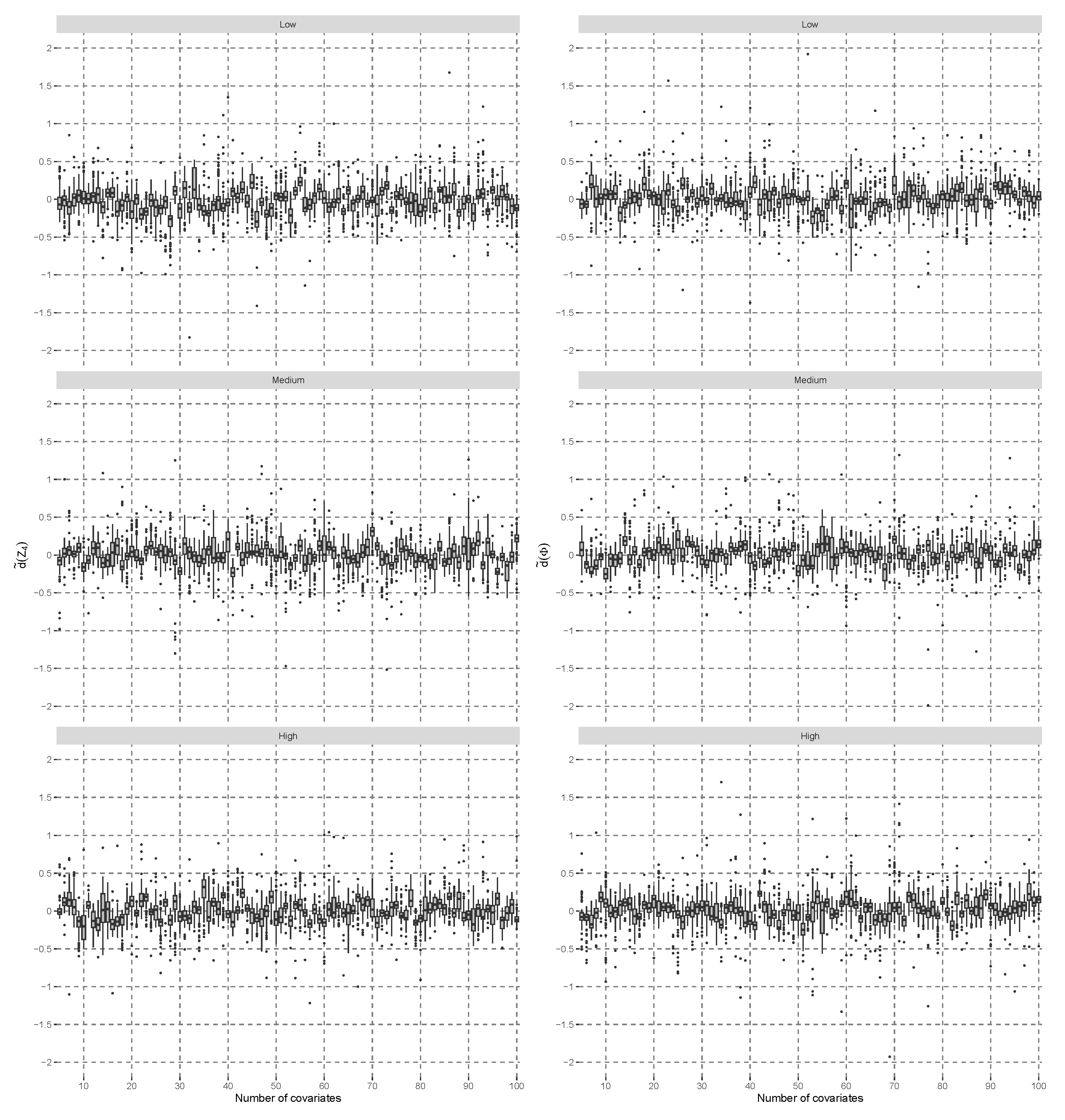
Here, the simulation results are shown for the null hypothesis that covariate one does not contribute to interaction effects ($s=\left\{1\right\}$). Figure 1 shows the difference $\tilde{d}\left({\widehat{z}}_4\right)$ defined by ${\widehat{z}}_4$, minus the normalized rank quantile of the standard normal distribution on the left side. $\tilde{d}\left({\widehat{z}}_4\right)$ was estimated based on 100 independent replicates of ${\widehat{z}}_4$, given the number of covariates and the correlation of each scenario. All boxplots fluctuate around the value of zero across different number of covariates. Furthermore, the boxplots on the left side, $\tilde{d}\left({\widehat{z}}_4\right)$, of Figure 1 are comparable to those on the right side, $\tilde{d}\left(\Phi \right)$, which used a standard, normal, distributed random variable, $\Phi$, instead of ${\widehat{z}}_4$. Note that the volatility in boxplots occurs due to the estimation of ranks, and with increasing sample sizes, the differences in $\tilde{d}\left(\Phi \right)$ would converge to zero. The Shapiro–Wilk test [36] is considered the most powerful in detecting non-normality according to [37]. If all 288 scenarios were evaluated with the Shapiro–Wilk test and adjusted for multiple comparisons with a false-discovery rate approach [38] of 0.05, then there would be no case that significantly departed from the normality distribution assumption.

The results for the alternative hypothesis specified in Equation (27) are shown in Figure 2. There is a decreasing trend to shift the distribution of ${\widehat{z}}_4$ more towards zero the higher the number of covariates. With low covariate correlation, the lower quartile of the distribution crosses the zero line with about 30 covariates. When the covariate correlation is higher, this happens with about 20 covariates. In such cases, it is expected that power is reduced because the $H_1$ distribution becomes more similar to the $H_0$ distribution. After about 30 covariates, the median of ${\widehat{z}}_4$ does not decrease further. For comparison, the same simulation was conducted using the t-statistic in a linear model of the interaction effect in Figure 3. This figure shows a decreasing trend in the location of the simulated t-value distribution, but the gap of the medians to zero is larger than in Figure 2, and more covariates are needed so that the lower quartile of the simulated distribution crosses the zero line. The model-specific hypothesis test that was explicitly developed for linear models can be expected to be more efficient in terms of power than a model-agnostic hypothesis test if the assumptions are justified. In conclusion, the proposed test statistic is empirically good when approximated with a normal distribution under $H_0$, and small effects under $H_1$ result in similar behavior to t-tests with linear models.

4.2. Power Simulation in Linear Models

This section focuses on the power and type I error simulation in linear models. Due to the linear structure of the models, interaction effects can be specified separately from main effects, and thus, simulations under both hypotheses $H_0$ and $H_1$ can be more easily specified and verified than in more complex prediction models. Therefore, the setting of linear models is a good starting point to explore the properties of the interaction test based on ${\widehat{z}}_4$. Note that, in practice, the proposed interaction test is not needed in linear models because ANOVA methods [23] were developed for the specific case of linear models to test whether the coefficients are zero.

The simulation design of the covariate distribution was the same as in the previous section, Section 4.1, with $p=5$, except additionally considering the case of no correlation. The data-generating model consisted of three different scenarios with the error term $ϵ\sim N(0,{\sigma }^2)$, and it was allowed to differ from the estimated prediction model specification:

$$\begin{array}{cc}\hfill & f\left(\mathit{x}\right)=\sum _{j=1}^p{\mathit{x}}_j{\mathit{\beta }}_j+ϵ(\mathrm{main}\mathrm{effects}),\hfill \\ \hfill & f\left(\mathit{x}\right)=\sum _{j=1}^p{\mathit{x}}_j{\mathit{\beta }}_j+\sum _{j=1}^{p-1}\sum _{k>j}{\mathit{x}}_j{\mathit{x}}_k{\mathit{\beta }}_{j,k}+ϵ(\mathrm{main}\mathrm{effects},\mathrm{all}\sec \mathrm{ond}\mathrm{order}\mathrm{interactions})\mathrm{and}\hfill \\ \hfill & f\left(\mathit{x}\right)=\sum _{j=1}^p{\mathit{x}}_j{\mathit{\beta }}_j+\sum _{j=1}^{p-1}\sum _{k>j}{\mathit{x}}_j{\mathit{x}}_k{\mathit{\beta }}_{j,k}+\sum _{j=1}^{p-2}\sum _{k>j}\sum _{l>j,l>k}{\mathit{x}}_j{\mathit{x}}_k{\mathit{x}}_l{\mathit{\beta }}_{j,k,l}+ϵ\hfill \\ \hfill & (\mathrm{main}\mathrm{effects},\mathrm{all}\sec \mathrm{ond}\mathrm{and}\mathrm{third}\mathrm{order}\mathrm{interactions}).\hfill \end{array}$$

The inference is about the population-model interaction effects (unknown in practice), but in this simulation, the interaction effects are known. The alternative hypothesis is true if the corresponding interaction effects are estimated in the prediction model and simulated in the data-generating process. In the case of the misspecification of the linear predictor, the estimated coefficients converge to the true coefficients of the data-generating process.

The error variance ${\sigma }^2$ was optimized on a data set with $n={10}^6$ prior to the simulation to approximately yield an explained variance of $0.25,0.5$, and $0.75$. Sample sizes varied with $n=\left\{100,125,\dots ,300\right\}$. Lower and upper sample sizes were chosen to avoid instabilities in the estimated coefficients and reach power levels of 1 in at least one scenario. Three different null hypotheses, $s=\left\{1\right\},\left\{1,2\right\},\left\{1,2,3\right\}$, were investigated. The linear model was specified under $H_1$ to estimate all possible main and interaction effects up to the third order. In contrast, under $H_0$ all interaction effects that included covariates of set s were excluded from the data-generating process. Each combination of the scenarios was repeated independently 1000 times.

The rows of plots in Section 4.2.1 and Section 4.2.2 correspond to different covariate correlations, $0,0.25,0.5,0.75$, and the columns of plots display varying explained variances, $0.25,0.5,0.75$. The dotted–dashed lines represent the upper and lower bounds of the exact pointwise $0.95$ Clopper–Pearson confidence intervals [39] that were calculated for the type I error and power proportions. The next two sections, Section 4.2.1 and Section 4.2.2, summarize the type I error and power simulation results consisting of $1.08\times {10}^6$ hypothesis tests. Additional figures are available in Supplementary Materials Section S4.

4.2.1. Type I Error Results

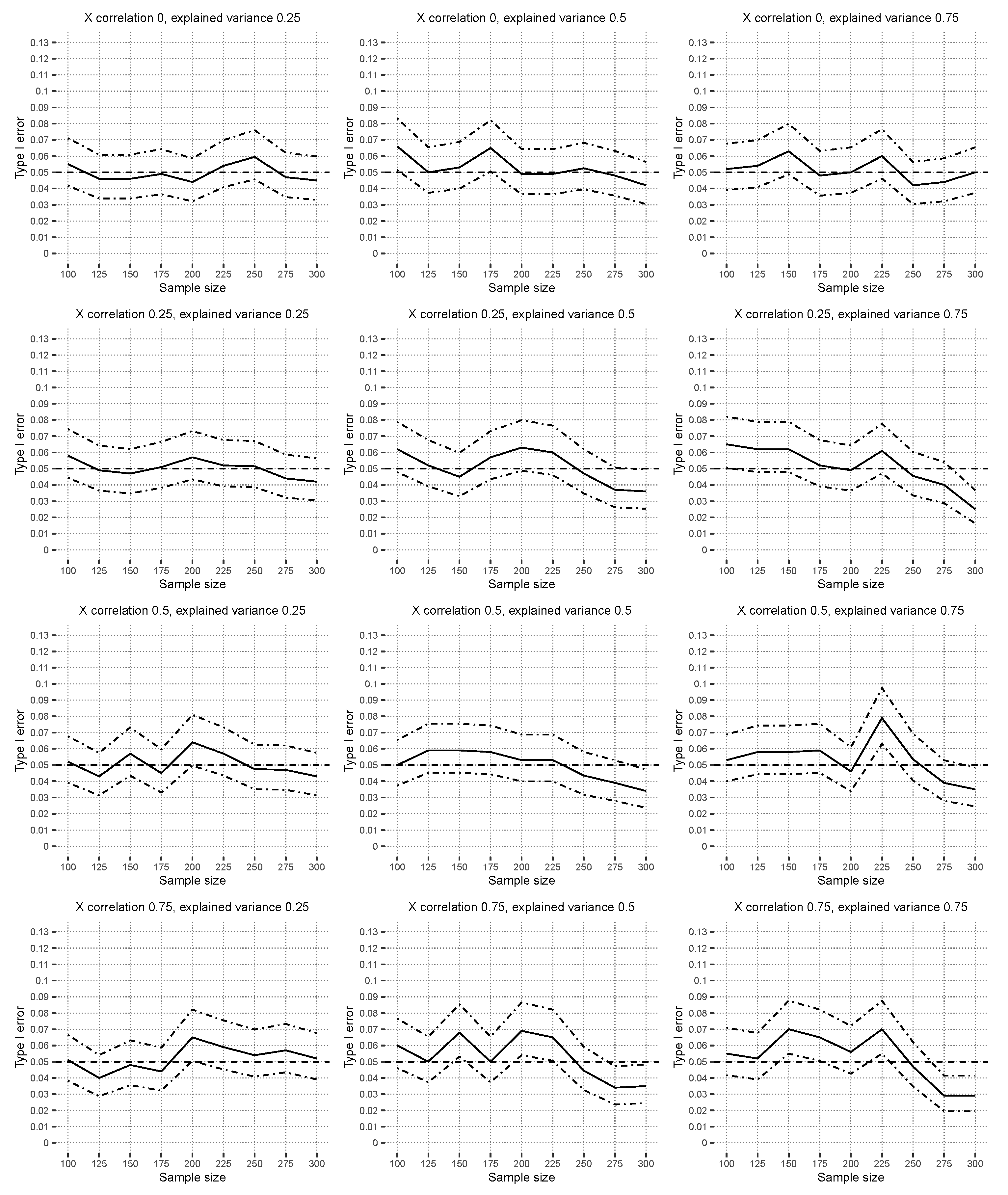
Figure 4 shows the results for the correctly specified linear model under $H_0$ with $s=\left\{1,2\right\}$. The estimated linear model includes the main effects of ${\mathit{x}}_{\left(1,2\right)}$ and additional interaction effects of the covariates ${\mathit{x}}_{\left(3,4,5\right)}$ up to the third order. The type I error was controlled with a significance level of $\alpha =0.05$ in all scenarios, and the hypothesis test is robust to covariate correlations, as well as explained variances.

4.2.2. Power Results

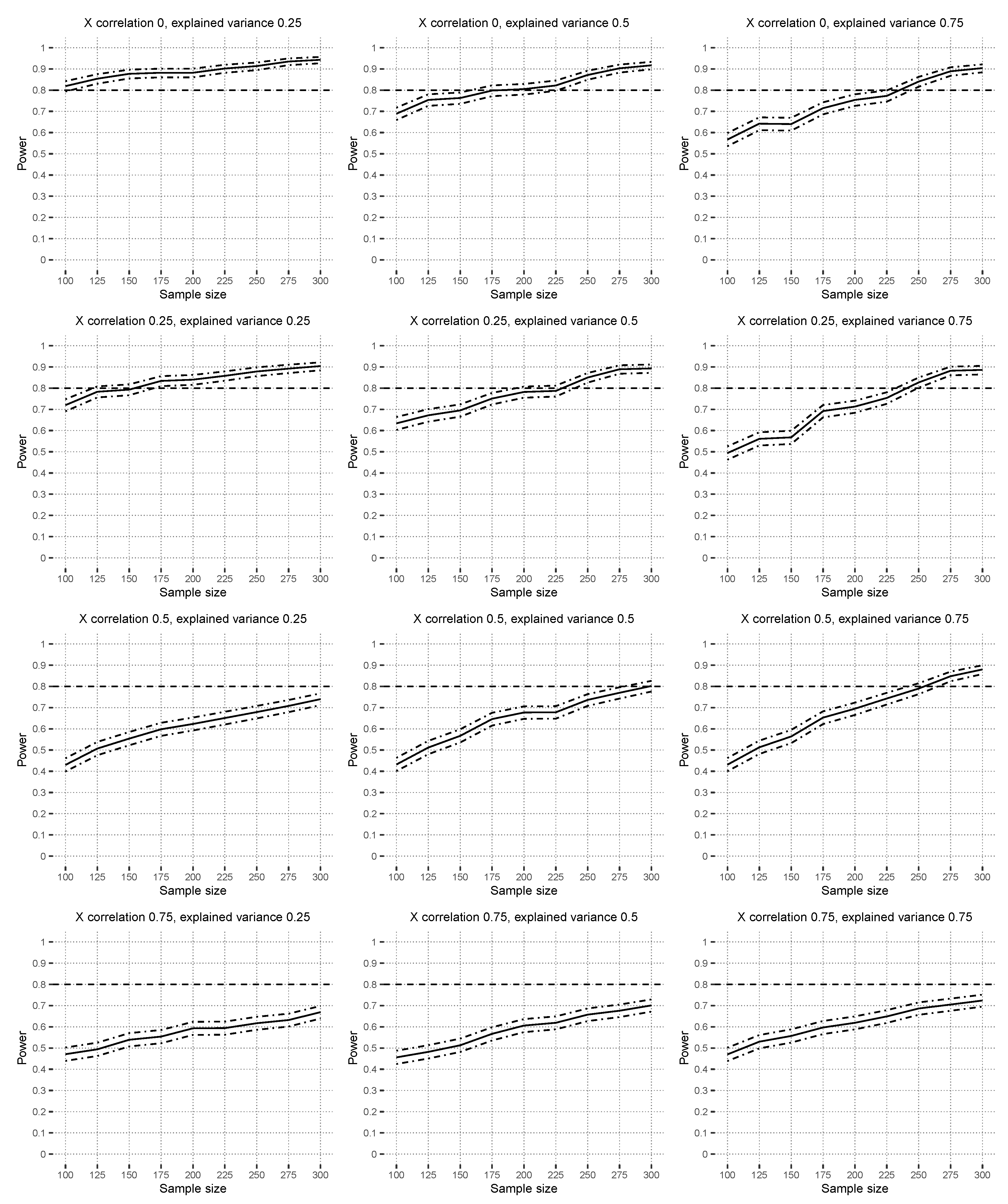
Figure 5 shows the power results under the alternative hypothesis based on $s=\left\{1,2\right\}$ with correctly specified linear models. The hypothesis test reaches power levels around $0.8$ in zero- to low-covariate correlation scenarios with at most $n=200$. The figure shows that higher covariate correlations reduce the power levels, which are influenced by the instability of the estimated linear models because of multicollinearity in this scenario. Higher explained variances result in slightly higher power. Note that the functional ANOVA decomposition theory [24] does not theoretically work well with strong covariate correlations either because great emphasis is placed on regions with a low probability mass [25].

Figure 6 shows the power results under $H_1$ with $s=\left\{1,2\right\}$ in the context of a misspecified linear model. The data-generating model consists of all interaction effects up to order two, except those in $s=\left\{1,2\right\}$, but in the linear model, the main effects and all possible interaction effects up to order three are estimated. Increasing covariate correlations reduces the power, and higher explained variance scenarios yield a higher power. Additional power scenarios are available in Supplementary Materials Section S4.2.

4.3. Power Simulation in Nonlinear Models

In this section, we aim to explore the power of the interaction test in a simulation study based on a data set. As an example data set, the credit approval data from the machine learning repository OpenML-CC18 [40,41] was used. The response variable was binary with categories for good and bad credit risks. The data set contains 1000 independent observations, along with 7 numeric and 13 categorical covariates. A descriptive overview of the data is given in Supplementary Materials Section S5.

The data-generating process of the simulation depends on the data set to be more realistic. Covariates were simulated without (Xind) and with dependencies (Xdep). In the former case, continuous covariates were randomly drawn from the marginal empirical distribution functions of one covariate. Discrete covariates were sampled according to observed relative frequencies. In the design Xdep, a Gaussian copula was used to simulate all continuous covariates together, considering their dependencies. The discrete covariate distribution was estimated using relative frequencies of multivariate contingency tables.

Ensemble methods like random forest were among the top-performing prediction methods with tabular data in a recent comparison to deep learning [42], and results from Kaggle competition challenges show similar trends (for example, [43]). Additionally, random forests are easy to tune, and usually, tuning the number of randomly available covariates at each split (mtry) suffices [44]. First, a random forest model was tuned via 10-fold cross-validation of the original data regarding out-of-sample, binomial log-likelihood function with the tuning parameter mtry (model ${\mathrm{RF}}_{\mathrm{interact}}$). Then, the absolute values of the interaction test statistic were evaluated for this model separately with each covariate. The three covariates with the highest values were chosen (age, employment, and existing credits). Among these sets, all possible pairwise sets with other covariates (excluding age, employment, and existing credits) were analyzed to determine the strongest two-way interaction effects in the data. These were “age of person interacts with housing finance”, “employment status interacts with housing finance”, and “number of existing credits interacts with job qualification”. The sets correspond to the covariates

$$\begin{array}{cc}\hfill & s=\left\{1\right\}\leftrightarrow “\mathrm{age}\mathrm{of}\mathrm{person}”\hfill \\ \hfill & s=\left\{1,2\right\}\leftrightarrow “\mathrm{age}\mathrm{of}\mathrm{person}”,“\mathrm{employment}\mathrm{status}”\hfill \\ \hfill & s=\left\{1,2,3\right\}\leftrightarrow “\mathrm{age}\mathrm{of}\mathrm{person}”,“\mathrm{employment}\mathrm{status}”,“\mathrm{number}\mathrm{of}\mathrm{existing}\mathrm{credits}”\hfill \end{array}$$

To evaluate the power and type I error rates, it is necessary to be able to specify the data-generating process under both the $H_0$ and $H_1$ hypotheses. It is known that, if the random forests are restricted to only include tree stumps (only one covariate split), then there are no interaction effects. In this simulation, all data-generation processes were identical to the specification of the estimated random forest models. Under $H_0$, all sets, s, were restricted to tree stumps depending on all covariates with the tuned parameter mtry (${\mathrm{RF}}_0$). For each strong interaction effect, separate random forests (${\mathrm{RF}}_{\mathrm{age},\mathrm{housing}},{\mathrm{RF}}_{\mathrm{employment},\mathrm{housing}},{\mathrm{RF}}_{\mathrm{credits},\mathrm{job}}$) were estimated with an unrestricted tree depth but only including the two variables of the previously determined interaction effect with $\mathrm{mtry}=2$. If there was a strong signal of two interaction covariates in the data and the random forest model had only the option to estimate the response with those covariates, then it was quite likely that the interaction effect would be estimated in the model. Under $H_1$ with set $s=\left\{1\right\}$, the predictions of ${\mathrm{RF}}_0$ and ${\mathrm{RF}}_{\mathrm{age},\mathrm{housing}}$ were averaged with the mean. Analogously, in the case of $s=\left\{1,2\right\}$, the random forest models ${\mathrm{RF}}_0,{\mathrm{RF}}_{\mathrm{age},\mathrm{housing}}$ and ${\mathrm{RF}}_{\mathrm{employment},\mathrm{housing}}$ were averaged, and if $s=\left\{1,2,3\right\}$, then the average predictions of ${\mathrm{RF}}_0,{\mathrm{RF}}_{\mathrm{age},\mathrm{housing}},{\mathrm{RF}}_{\mathrm{employment},\mathrm{housing}}$ and ${\mathrm{RF}}_{\mathrm{credits},\mathrm{job}}$ were calculated. After data generation, the estimated random forest models were tuned using simulated test data analogously as model ${\mathrm{RF}}_{\mathrm{interact}}$. All together, there were 120 scenarios (10 sample sizes, two covariate designs, three sets s, and two different hypotheses) that were independently repeated 1000 times.

4.3.1. Type I Error Results

In Figure 7, the estimated type I errors, based on random forests, are shown for independent covariate simulation. The curves fluctuate around the prespecified alpha level of $0.05$. In the case of dependent covariates, Figure 8 shows that the type I error is controlled for $s=\left\{1\right\}$. Larger sets indicate a small positive trend for increasing sample sizes. This could indicate that covariate dependencies have a small influence on the type I error in nonlinear models. This is in contrast to the observed results of Section 4.2.1, where even strong covariate correlations overall did not have much of an effect on the estimated type I errors. In the design Xdep, the strongest correlation in the Gaussian copula between “credit amount” and “credit duration” was $0.6174$ in the original data set. All other numeric covariates had less absolute correlation than $0.3$. The simulated interaction effect between “employment” and “housing finance”, measured using the corrected contingency coefficient [45], was $0.2909$. The previous value is above the $0.95$ empirical simulated quantile $0.1527$ under independence, and thus, this case can be interpreted as low-dependency. Another difference compared to linear models is that random forests do not have continuous predictions, which means that, for certain ranges of the covariates, the prediction function stays constant.

4.3.2. Power Results

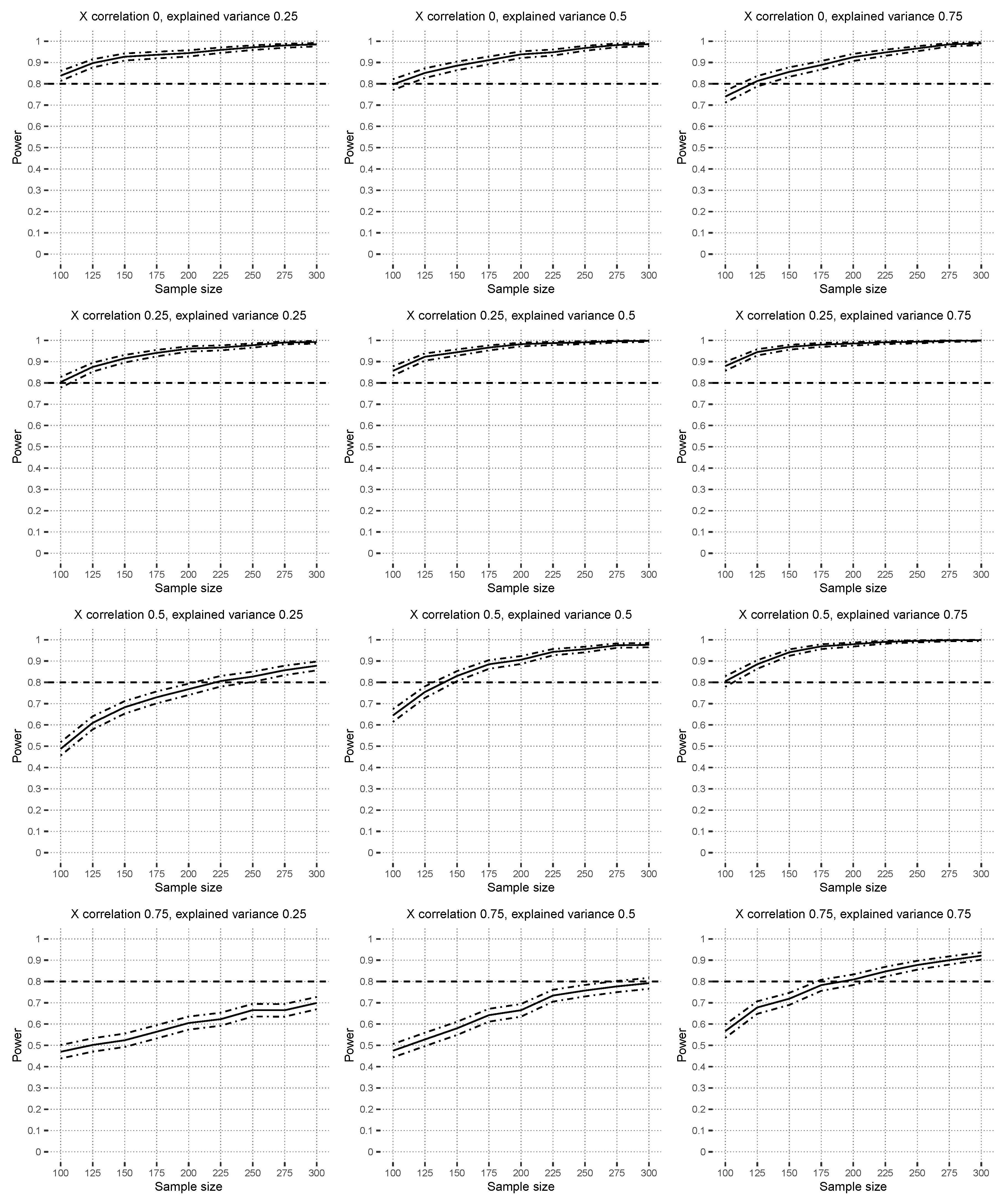
Figure 9 shows the estimated power based on random forest models. Power increases with the sample size, and the curve gradients decline. Several hundred observations are sufficient to ensure commonly used power levels of $0.8$ [46]. In contrast to Figure 9, the scenarios of $∥s∥>1$ in Figure 10 show somewhat lower power levels at sample size $n=1000$. It is analogous to the previous section, Section 4.3.1, that the performance using the Xdep design is a little bit worse than that using the Xind design.

4.4. Interaction Test Statistic with Response

In this section, we explore the proposed extension in Equation (25) to include response information in ${\widehat{z}}_{P,4}$ as a sensitivity analysis. The simulation design was based on the example given in [27,47]. The response function takes the form of $H_0$

$$\begin{array}{cc}\hfill & g\left(\mathit{x}\right)=5sin\left(\pi {\mathit{x}}_1\right)+5sin\left(\pi {\mathit{x}}_2\right)+20{\left({\mathit{x}}_3-0.5\right)}^2+10{\mathit{x}}_4+5{\mathit{x}}_5+ϵ\mathrm{and}\mathrm{under}{H}_1\hfill \end{array}$$

(28)

$$\begin{array}{cc}\hfill & g\left(\mathit{x}\right)=10sin\left(\pi {\mathit{x}}_1{\mathit{x}}_2\right)+20{\left({\mathit{x}}_3-0.5\right)}^2+10{\mathit{x}}_4+5{\mathit{x}}_5+ϵ\hfill \end{array}$$

(29)

with $\mathit{x}\in {\mathbb{R}}^{10}$ and $ϵ\sim N\left(0,{\sigma }^2\right)$. Both under $H_0$ and $H_1$, the error variance was set to achieve an explained variance of 95% based on the average of 25 independent simulated data sets of size ${10}^6$. The sample sizes varied from $n=100,200,\dots ,1000$. For each simulated training data set, a multivariate adaptive regression spline (MARS) was fitted [47] with a maximal degree of two. 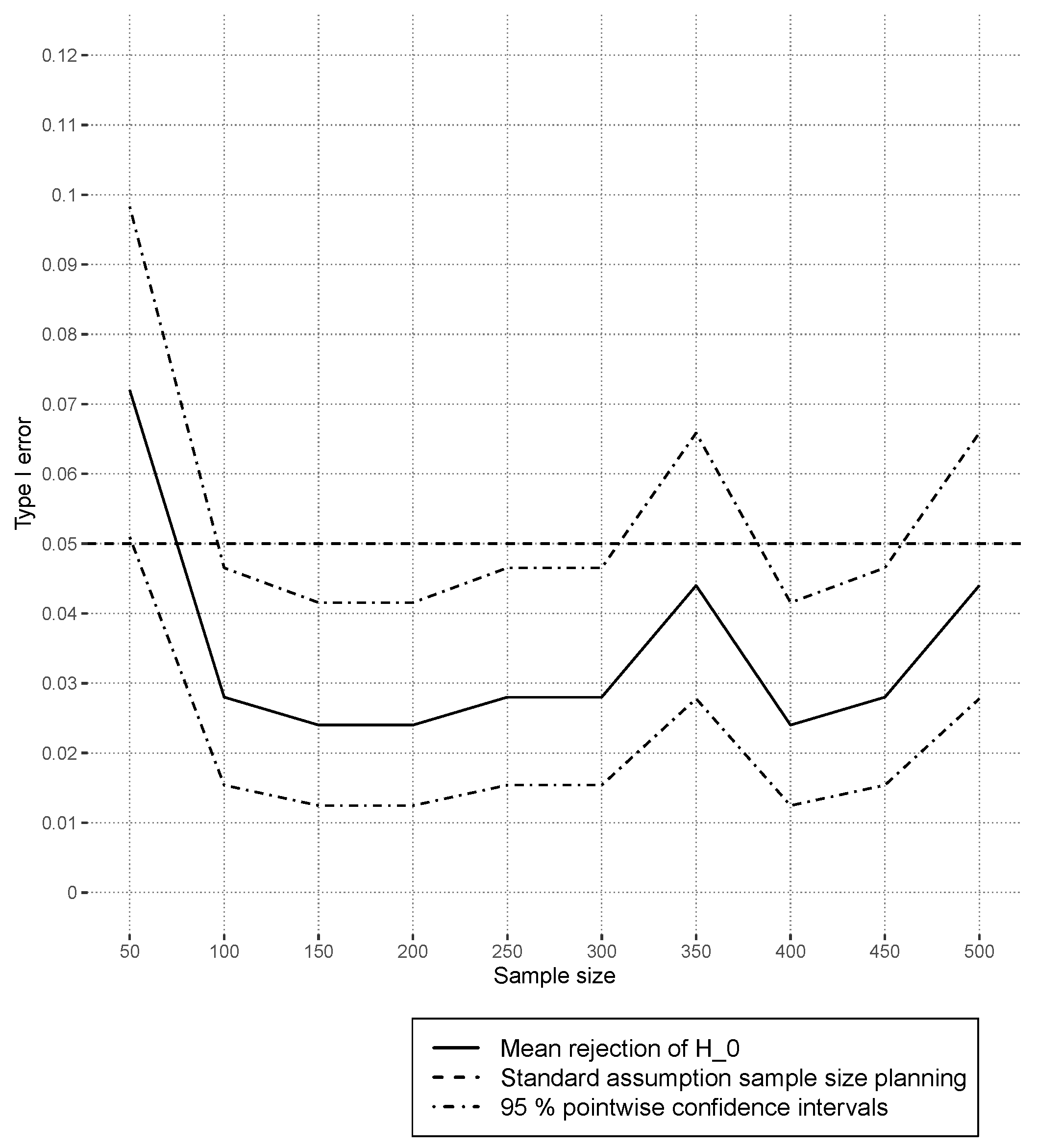Type I error results are shown in Figure 11. 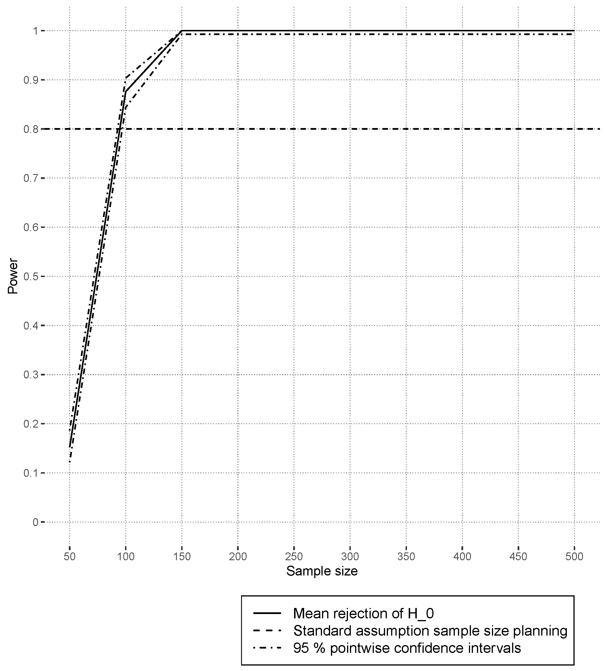Overall, the estimated type I error held the specified alpha level $0.05$, but it was slightly conservative. In this example, at least 100 observations were sufficient to achieve power levels above 80% (Figure 12). The results demonstrate that the modified test statistic with the response information ${\widehat{z}}_{P,4}$ is also able to control the type I error, and it achieves reasonable power levels similar to ${\widehat{z}}_4$.

5. Data Analysis

This section summarizes the results of the data analysis example. The Boston Housing prices data set from the US census in 1970 [48] was explored for comparison to the data set investigated by [22]. The median value of owner-occupied homes in 1000s of USD was the quantitative response. All available other variables were used as covariates in an extreme gradient-boosting model [49]. The data set was split randomly into tuning data (50%) and a test data set (50%). The tuning data were split again with five times repeated 25-fold cross-validation to tune all possible pairs of the number of boosting iterations $1000,1100,\dots ,2000$ and the maximal tree depth $1,2,\dots ,14$. The learning rate was set constant to $0.01$, and subsampling of the rows and columns was done with a probability of $0.5$. The tuning parameters with the lowest MSE were 2000 boosting iterations and a tree depth of 4. Let the performance measure $\xi \left(M\right)$ be the average absolute prediction error of the model M divided by the average absolute prediction error of the median response. Evaluating $\xi \left(M\right)$ on the test set with the model results in $0.4323$. Note that the mean of $\xi \left(M\right)$ over all tuning grid values, $0.3407$, was comparable to the results of [22]. Testing the null hypothesis of no interaction between all covariates gave a p-value of $0.0107$. Thus, interaction effects have an impact. 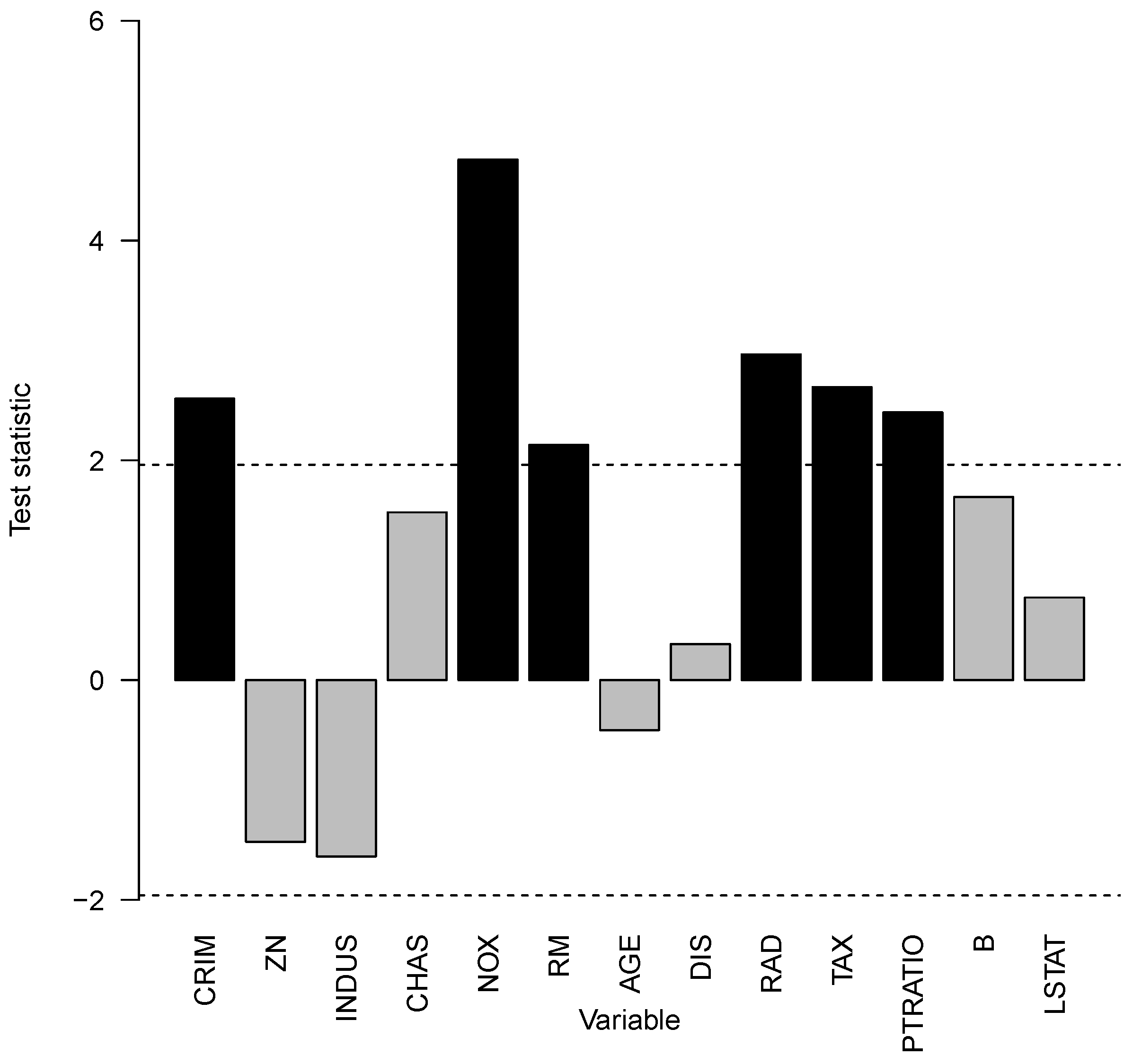To assess which covariates contribute to interaction effects, all sets $\left[s=\left\{1\right\},s=\left\{2\right\},\dots ,s=\left\{14\right\}\right]$ were investigated in Figure 13. All covariates above or below the dashed line per capita crime rate by town (CRM), nitric oxides concentration with parts per 10 million (NOX), average number of rooms per dwelling (RM), index of accessibility to radial highways (RAD), full-value property tax rate per 10,000 USD (TAX), and the pupil–teacher ratio by town (PTRATIO) contribute to interaction effects for Boston housing prices. All of those covariates have positive values for the test statistic, which means that those interaction effects overall increase the variability of the prediction model.

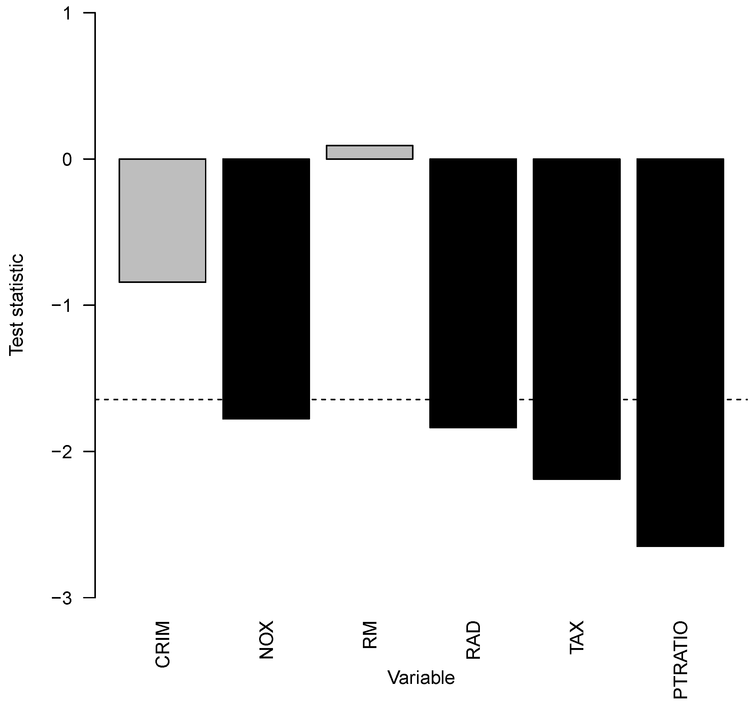
In the next step, the impact of the previously identified covariate interaction effects can be evaluated. First, covariates with interaction effects $s=\left\{1,5,6,9,10,11\right\}$ were tested one-sided with the null hypothesis that the prediction model with possible interaction effects has an equal or higher MSE. Overall, the p-value was $0.0155$, and we concluded that the interaction effects of those covariates reduce the MSE. The MSE was reduced by 5.46% relative to the prediction model without interaction effects. The next question is: Which interaction effects associated covariates are responsible for this reduction? It is answered in Figure 14. In this particular case of Boston housing prices, interaction effects with covariates NOX, RAD, TAX, and PTRATIO led to statistically significant MSE improvements in the prediction model. This means that the covariates influence the Boston Housing prices with two-way or higher-order interaction effects, and those identified interaction effects improve the prediction performance.

6. Discussion

This work introduced a model-agnostic statistical interaction test that a hypothesis set can be flexibly specified. An asymptotic distribution of the test statistic was derived (Section 3). The interaction test neither required the refitting of the prediction model nor the resampling of the original data. The low computational runtime cost of the interaction test allows for the exploration of multiple sets of covariates. Our recommendation is to evaluate the test statistic with test data. The distribution of the test statistic behaved well in linear models even in the case of strong covariate correlations (Section 4.1). Simulations with linear (Section 4.2) and nonlinear models (Section 4.3) show that, overall, the type I error is bounded by the prespecified alpha level in most cases and that the test achieves reasonable power levels for several hundred observations in the simulations. The interaction test can be used for black-box models along with other measures of interpretability to better understand interaction effects. Low deviations of the test statistic from zero may indicate that the prediction model could be approximated well using a simpler model without covariate interaction effects in set s.

In addition to Section 3, the evaluation of ${\widehat{z}}_4$ under the training data ${\mathit{X}}_1,{\mathit{X}}_2,\dots ,{\mathit{X}}_n$ was discussed. In this case, the observations ${\widehat{z}}_{3,1},{\widehat{z}}_{3,2},\dots ,{\widehat{z}}_{3,n}$ are dependent because each observed value of ${\widehat{z}}_{3,i}$ includes all training data in the estimation of the PD function in ${\widehat{z}}_{1,i},{\widehat{z}}_{2,i}$. The prediction model $\widehat{f}\left(\mathit{x}\right)$ is not constant and changes if the training sample size increases because it is estimated from the same data. As such, the uniform convergence speed of $\widehat{f}\left(\mathit{x}\right)$ and the PD functions $\widehat{\mathrm{PD}}\left({\mathit{x}}_s\right)$ would need to be faster than $n^{-1/2}$, which corresponds to the convergence speed of the mean according to the Berry–Essens theorem (see, for example, [50]). However, especially nonparametric machine learning models usually have a lower convergence speed than $n^{-1/2}$ [51], and there is no guarantee that multiplications of ${\widehat{z}}_1,{\widehat{z}}_2$ in ${\widehat{z}}_3$ yield faster convergence rates. Additionally, the CLT would require extensions to work under dependence between observations such as those presented in [52,53]. That specific theory would require the supremum of the maximal correlation coefficient (SMCC) [54] for all possible sets of observations ${\widehat{z}}_{3,i_1},{\widehat{z}}_{3,i_2}$ with lag $\mathcal{L}=\left|i_1-i_2\right|$ to converge at least linearly to zero as $\mathcal{L}\to \infty$. This assumption is difficult to investigate with simulations and, to the best of the authors’ knowledge, impossible to prove because the number of available observations with a specific lag depends on the sample size, while the supremum of the maximal correlation depends on the number of comparisons. Note that, in the case of iid random variables, higher dimensions of the covariate matrix (more comparisons) affect the distribution of the maximal estimated Pearson correlation (see [55] for asymptotic results).

Whether to use ${\widehat{z}}_4$ or ${\widehat{z}}_{P,4}$ with a response should be decided according to the goals of data analysis. The choice may also consider the characteristics of the data-generating process of the application. For example, if the signal-to-noise ratio is low, then ${\widehat{z}}_4$ would be preferable to ${\widehat{z}}_{P,4}$ regarding statistical power because, in this case, the usage of the response information would add more noise that would make it harder to differentiate between $H_0$ and $H_1$. In the reverse situation with a high signal-to-noise ratio, the additional information of the response in ${\widehat{z}}_{P,4}$ could reduce the variability of the terms ${\mathrm{IADP}}_{f,s}$ and ${\mathrm{IADP}}_{PD,s}$, and thus, hypotheses $H_0$ and $H_1$ could be more easily distinguished compared to the test statistic ${\widehat{z}}_4$. Future research may investigate the behavior of both statistics, ${\widehat{z}}_4,{\widehat{z}}_{4}P,4$, in other settings that were not considered in this work (for example, other data sets and different black-box prediction models).

From a general perspective, the choice of whether to apply IML to training or test data depends on the goals of statistical analysis [56]. If the influence of covariates on the prediction model at the population level is the focus of interest, it does not matter whether training or test data are used, as long as data sets originate from the same data-generating process. The more data are available, the more powerful the proposed interaction test is, provided that all other conditions stay constant. In contrast, if the goal is to analyze the impact of covariates on prediction performance, then it is reasonable to apply IML methods to test data sets. This is in line with [18], who recommends the usage of test data in the case of permutation variable importance. Test data usage in the interaction difference test has better theoretical properties and, thus, is recommended for applications.

An alternative to ${\mathrm{H}}_s^2$ was proposed by [57] that uses accumulated local effect functions instead of PD functions. ALE curves are more computationally efficient and avoid the extrapolation problem to non-observed covariate combinations. However, ALE curves attribute part of the interaction effect to the main effect if there are interactions between correlated features [58]. Extrapolations can be investigated graphically via the stratification of PD plots regarding other covariates. Furthermore, PD plots can be enhanced using individual conditional expectation curves [28], which plot each observed predicted value to investigate variability and possible interaction effects. This graphical representation is not available for ALE. Therefore, this paper focused on the analysis of PD functions.

7. Conclusions

This work has proposed a new model-agnostic hypothesis test to detect interaction effects in prediction models. The null hypothesis states that a given set of covariates does not contribute to any interaction effects. The concept is based on the interaction difference between the variances of the original model predictions and predictions under restricted interaction effects with the null hypothesis. The restricted form of the prediction model is given via functional ANOVA decomposition, combined with partial dependence functions. The interaction difference was then embedded into the framework of a two-sided, one-sample Z-test. The resulting test statistic is asymptotically normally distributed if it is evaluated using test data. Various simulations showed that, in most cases, the type I error was controlled, and several hundred observations yielded reasonable power levels.

The extended test statistic ${\widehat{z}}_{P,4}$ was explored to incorporate response information into ${\widehat{z}}_4$. If interaction effects were detected with ${\widehat{z}}_4$, the modification ${\widehat{z}}_{P,4}$ could be used to assess whether these interaction effects contributed to MSE prediction performance. In this case, the null hypothesis is that the MSE of the original model with interaction effects is equal to or worse than the prediction model without those interaction effects.

Overall, this work has extended the existing IML methodology to better explain black-box prediction models’ interaction effects. It is computationally run time-efficient due to the derived asymptotic distribution and available on CRAN as the R-package IADT.