An Analysis of Radio Frequency Transfer Learning Behavior

Abstract

Transfer learning (TL) techniques, which leverage prior knowledge gained from data with different distributions to achieve higher performance and reduced training time, are often used in computer vision (CV) and natural language processing (NLP), but have yet to be fully utilized in the field of radio frequency machine learning (RFML). This work systematically evaluates how the training domain and task, characterized by the transmitter (Tx)/receiver (Rx) hardware and channel environment, impact radio frequency (RF) TL performance for example automatic modulation classification (AMC) and specific emitter identification (SEI) use-cases. Through exhaustive experimentation using carefully curated synthetic and captured datasets with varying signal types, channel types, signal to noise ratios (SNRs), carrier/center frequencys (CFs), frequency offsets (FOs), and Tx and Rx devices, actionable and generalized conclusions are drawn regarding how best to use RF TL techniques for domain adaptation and sequential learning. Consistent with trends identified in other modalities, our results show that RF TL performance is highly dependent on the similarity between the source and target domains/tasks, but also on the relative difficulty of the source and target domains/tasks. Results also discuss the impacts of channel environment and hardware variations on RF TL performance and compare RF TL performance using head re-training and model fine-tuning methods.

1. Introduction

Radio frequency machine learning (RFML) is loosely defined as the application of deep learning (DL) to raw RF data and has yielded state-of-the-art algorithms for spectrum awareness, cognitive radio, and networking tasks. Existing RFML works have delivered increased performance and flexibility and reduced the need for pre-processing and expert-defined feature extraction techniques. As a result, RFML is expected to enable greater efficiency, lower latency, and better spectrum efficiency in 6G systems [1]. However, to date, little research has considered and evaluated the performance of these algorithms in the presence of changing hardware platforms and channel environments, adversarial contexts, or resource constraints that are likely to be encountered in real-world systems [2].

Current state-of-the-art RFML techniques rely upon supervised learning techniques trained from random initialization, and thereby assume the availability of a large corpus of labeled training data (synthetic, captured, or augmented [3]), which is representative of the anticipated deployed environment. Over time, this assumption inevitably breaks down as a result of changing hardware and channel conditions, and as a consequence, performance degrades significantly [4,5]. TL techniques can be used to mitigate these performance degradations by using prior knowledge obtained from a source domain and task, in the form of learned representations, to improve performance on a “similar” target domain and task using less data, as depicted in Figure 1.

Though TL techniques have demonstrated significant benefits in fields such as CV and NLP [6,7,8,9], including higher performing models, significantly less training time, and far fewer training samples [10,11] showed that the use of TL in RFML is currently lacking through the construction of an RFML specific TL taxonomy. 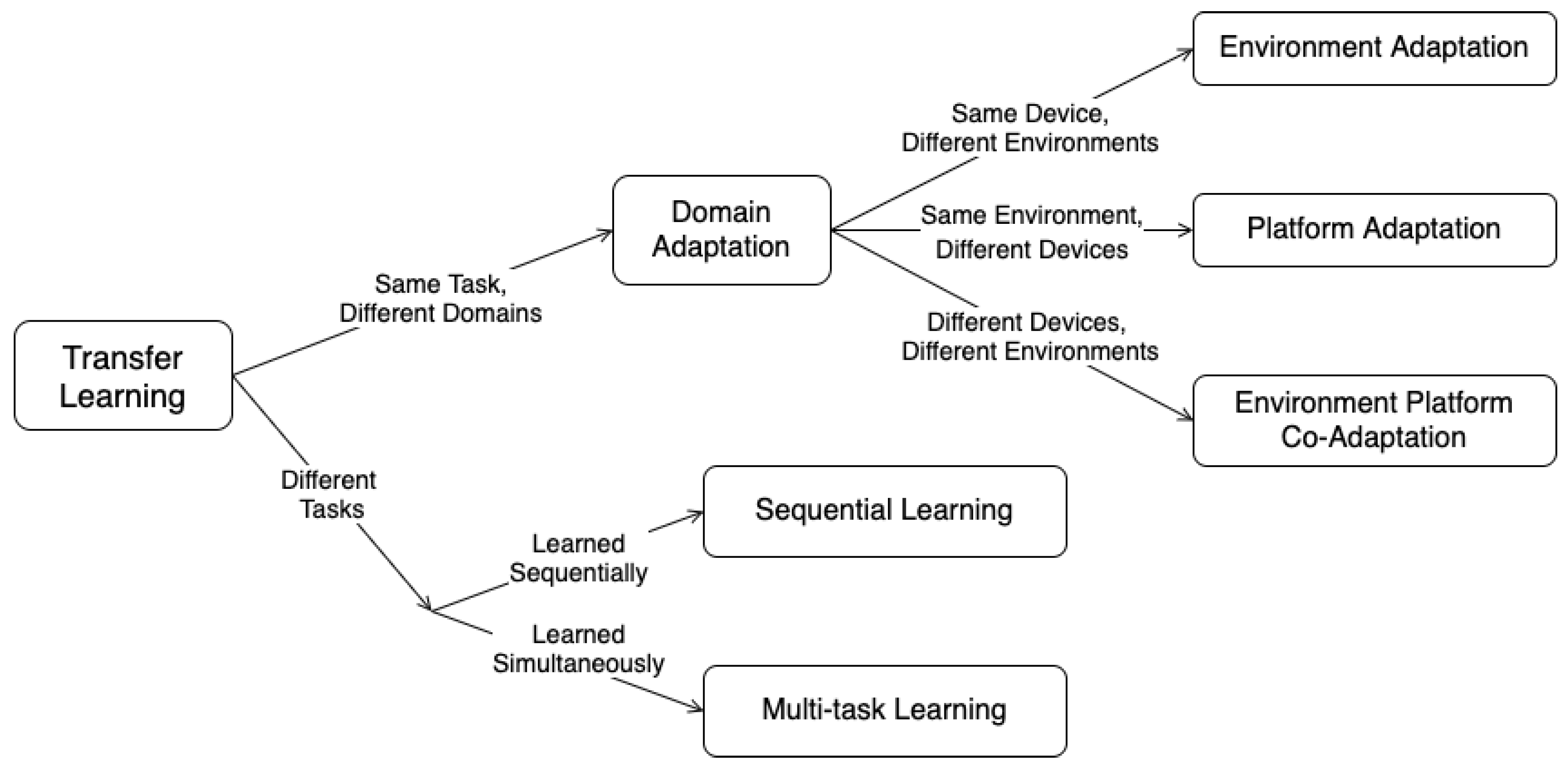This work begins to address current limitations in understanding how the training domain and task impact learned behavior and therefore facilitate or prevent successful transfer, where the training domain is characterized by the RF hardware and the channel environment [11] depicted in Figure 2 and the training task is the application being addressed including the range of possible outputs (i.e., the modulation schemes classified). More specifically, this work systematically evaluates RF TL performance, as measured by post-transfer top-1 accuracy, as a function of several parameters of interest for example AMC [4] and SEI use-cases [12] using synthetic and captured datasets.

From these experiments, we identify a number of practical takeaways for how best to utilize TL in an RFML setting including how changes in propagation environment, Tx/Rx hardware, and CF impact the difficulty of AMC and SEI. We also examine head re-training versus fine-tuning performance for RF TL, and discuss methods for predicting RF TL performance including using dataset similarity and existing transferability metrics. These takeaways, verified across different RFML use-cases and DL architectures using both synthetic and captured data, serve as initial guidelines for RF TL.

This paper is organized as follows: Section 2 provides requisite background knowledge of TL and RFML. In Section 3, each of the key methods and systems used and developed for this work are described in detail, including data generation and collection set-ups, dataset creation, and model architectures and training. Section 4 presents the experimental results and analysis, and finally, Section 5 offers conclusions about the effectiveness of TL for RFML and the next steps for incorporating and extending TL techniques in RFML-based research. A list of the acronyms used in this work is provided in the appendix for reference.

2. Background

The following subsections provide an overview of RFML, TL, and TL for RFML to provide context for the work performed herein.

2.1. Radio Frequency Machine Learning (RFML)

The term RFML is often used in the literature to describe any application of machine learning (ML) or DL to the RF domain. However, RFML was coined by Defense Advanced Research Projects Agency (DARPA) and is defined as systems that:

• Autonomously learn features from raw data to detect, characterize, and identify signals of interest;
• Can autonomously conFigure RF sensors or communications platforms for changing communications environments;
• Can synthesize “any possible waveform” [13].

Therefore, RFML algorithms typically utilize raw RF data as input to ML/DL techniques, most often deep neural networks (DNNs).

To date, most RFML research has focused on delivering state-of-the-art performance on spectrum awareness and cognitive radio tasks, whether through increased accuracy, increased adaptability, or using less expert knowledge. Such spectrum awareness cognitive radio tasks include signal detection, signal classification or AMC, SEI, channel modeling/emulation, positioning/localization, and spectrum anomaly detection [2]. One of the most common and arguably the most mature spectrum awareness or cognitive radio applications explored in the literature is AMC, which is the task of identifying the type or format of a detected signal, which is a key step in receiving RF signals. Meanwhile, SEI is the task of identifying the unique Tx responsible for sending a signal of interest. Both traditional AMC and SEI techniques have typically consisted of an expert-defined feature extraction stage followed by a pattern recognition stage, such as a decision tree, support vector machine, or multi-layer perceptron (MLP) [14,15]. RFML-based approaches aim to both automatically learn and identify key features within signals of interest, as well as utilize those features to perform various tasks, using only minimally pre-processed raw RF as an input to DNN architectures including convolutional neural networks (CNNs) and recurrent neural networks (RNNs) [16,17].

2.2. Transfer Learning (TL) for RFML

As previously mentioned, TL aims to utilize prior knowledge gained from a source domain/task to improve performance on a “similar” target domain/task, where training data may be limited. The domain, $D=\{X,P(X\left)\right\}$, consists of the input data X and the marginal probability distribution over the data $P\left(X\right)$. Meanwhile, the task, $T=\{Y,P(Y\left|X\right)\}$, consists of the label space Y, and the conditional probability distribution $P\left(Y\right|X)$ learned from the training data pairs $\{x_i,y_i\}$ such that $x_i\in X$ and $y_i\in Y$. In the context of RFML, the domain is characterized by the RF hardware and channel environments (i.e., in-phase/quadrature (IQ) imbalance, non-linear distortion, SNR, multi-path effects), and the task is the application being addressed, including the range of possible outputs (i.e., n-class AMC, SEI, SNR estimation).

Recent work presented the RF-specific TL taxonomy shown in Figure 3 [11], adapted from the general TL taxonomy of [18] and the NLP-specific taxonomy of [19]. Per this taxonomy, RF TL is categorized by training data availability and whether or not the source and target tasks differ:

• Domain adaptation is the setting in which source and target tasks are the same, but the source and target domains differ, and can be further categorized as follows:

  -

  Environment adaptation, where the channel environment is changing, but the Tx/Rx pair(s) are constant;

  -

  Platform adaptation, where the Tx/Rx hardware is changing, but the channel environment is consistent;

  -

  Environment platform co-adaptation, where changes in both the channel environment and Tx/Rx hardware must be overcome.

• Multi-task learning is the setting in which different source and target tasks are learned simultaneously.
• Sequential learning is the setting in which a source task is learned first, and the target task, different from the source task, is learned during a second training phase.

Typically, the same training techniques are used to perform both domain adaptation and sequential learning, most commonly head re-training and model fine-tuning, which are the focus of this work. Existing works have successfully utilized such techniques to overcome changes in the channel environment [20,21] and wireless protocol [12,22], to transfer from synthetic data to captured data [23,24,25], and to add or remove output classes [26], for a variety of RFML use-cases. Meanwhile, multi-task learning approaches tend to utilize more than one loss term during a single training phase and have been more commonly used in the context of ML-enabled wireless communications systems that use expert-defined features rather than raw RF data as input. However, multi-task learning techniques have been used to facilitate end-to-end communications systems [27], as well as to improve the explainability and accuracy of RFML models [28]. A systematic examination and evaluation of multi-task learning performance is left for future work.

Outside of observing the inability of pre-trained RFML models to generalize to new domains/tasks [3,4,29], little to no work has examined what characteristics within RF data facilitate or restrict transfer [11]. Without such knowledge, TL algorithms for RFML are generally restricted to those borrowed from other modalities, such as CV and NLP. While correlations can be drawn between the vision or language spaces and the RF space, these parallels do not always align, and therefore algorithms designed for CV and NLP may not always be appropriate for use in RFML. For example, while CV algorithm performance is not significantly impacted by a change in the camera(s) used to collect data, so long as the image resolution remains consistent [30], work in [4] showed that a change in Tx/Rx pairs negatively impacted performance by as much as 7%, despite the collection parameters and even the brand/models of Txs/Rxs remaining consistent. Therefore, platform adaptation techniques that transfer knowledge gleaned from one hardware platform (or set of platforms) to a second hardware platform (or set of platforms) are a necessity in RFML, but not in CV.

3. Methodology

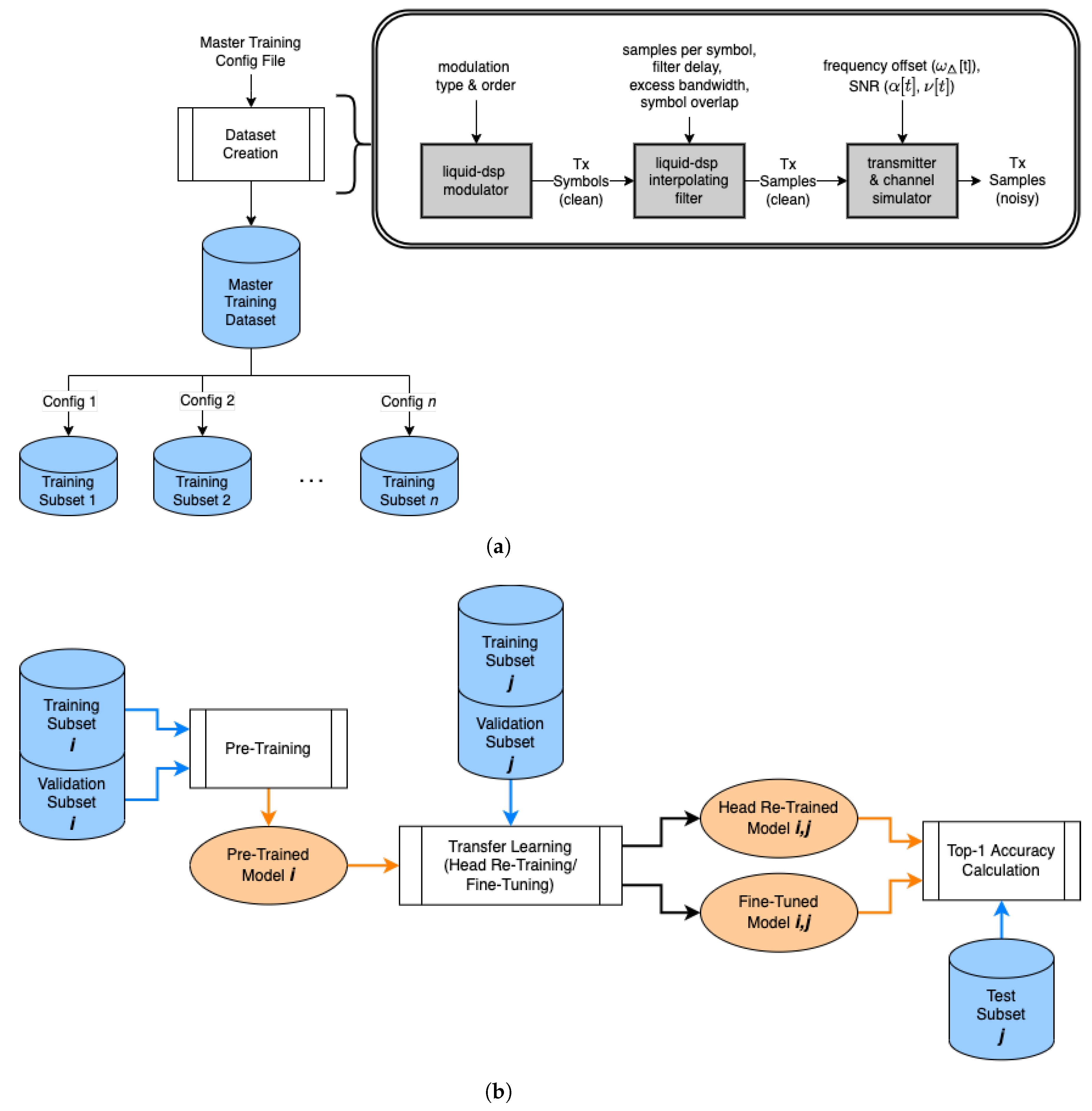
This section presents the experimental setup used in this work, shown in Figure 4, which includes the data generation and collection processes, the dataset creation process, model architectures, and training evaluation, each described in detail in the following subsections.

3.1. Synthetic Data Generation

All synthetically generated data used in this work was created using a python wrapper around the open-source signal processing library liquid-dsp [31], which allowed for full control over the chosen parameters of interest, SNR, FO, and modulation type, and ensured accurate labeling of the training, validation, and test data. Additionally, the synthetic data used in this work was generated using the same noise generation, signal parameters, and signal types as in [28], such that the signal space has been restricted to the 23 signal types shown in

Table 1. Signal types included in this work and generation parameters. All abbreviations are defined at the end of the document.

Modulation Name	Parameter Space
BPSK	Symbol Order {2} RRC Pulse Shape Excess Bandwidth {0.35, 0.5} Symbol Overlap ∈ [3, 5]
QPSK	Symbol Order {4} RRC Pulse Shape Excess Bandwidth {0.35, 0.5} Symbol Overlap ∈ [3, 5]
PSK8	Symbol Order {8} RRC Pulse Shape Excess Bandwidth {0.35, 0.5} Symbol Overlap ∈ [3, 5]
PSK16	Symbol Order {16} RRC Pulse Shape Excess Bandwidth {0.35, 0.5} Symbol Overlap ∈ [3, 5]
OQPSK	Symbol Order {4} RRC Pulse Shape Excess Bandwidth {0.35, 0.5} Symbol Overlap ∈ [3, 5]
QAM16	Symbol Order {16} RRC Pulse Shape Excess Bandwidth {0.35, 0.5} Symbol Overlap ∈ [3, 5]
QAM32	Symbol Order {32} RRC Pulse Shape Excess Bandwidth {0.35, 0.5} Symbol Overlap ∈ [3, 5]
QAM64	Symbol Order {64} RRC Pulse Shape Excess Bandwidth {0.35, 0.5} Symbol Overlap ∈ [3, 5]
APSK16	Symbol Order {16} RRC Pulse Shape Excess Bandwidth {0.35, 0.5} Symbol Overlap ∈ [3, 5]
APSK32	Symbol Order {32} RRC Pulse Shape Excess Bandwidth {0.35, 0.5} Symbol Overlap ∈ [3, 5]
FSK5k	Carrier Spacing {5 kHz} Rect Phase Shape Symbol Overlap {1}
FSK75k	Carrier Spacing {75 kHz} Rect Phase Shape Symbol Overlap {1}
GFSK5k	Carrier Spacing {5 kHz} Gaussian Phase Shape Symbol Overlap {2, 3, 4} Beta ∈ [0.3, 0.5]
GFSK75k	Carrier Spacing {75 kHz} Gaussian Phase Shape Symbol Overlap {2, 3, 4} Beta ∈ [0.3, 0.5]
MSK	Carrier Spacing {2.5 kHz} Rect Phase Shape Symbol Overlap {1}
GMSK	Carrier Spacing {2.5 kHz} Gaussian Phase Shape Symbol Overlap {2, 3, 4} Beta ∈ [0.3, 0.5]
FM-NB	Modulation Index ∈ [0.05, 0.4]
FM-WB	Modulation Index ∈ [0.825, 1.88]
AM-DSB	Modulation Index ∈ [0.5, 0.9]
AM-DSBSC	Modulation Index ∈ [0.5, 0.9]
AM-LSB	Modulation Index ∈ [0.5, 0.9]
AM-USB	Modulation Index ∈ [0.5, 0.9]
AWGN

, observed at complex baseband in the form of discrete time-series signals, s[t], where

$$s\left[t\right]={\alpha }_{\Delta }\left[t\right]·\alpha \left[t\right]e^{\left(j\omega \right[t]+j\theta [t\left]\right)}·e^{(j{\omega }_{\Delta }\left[t\right]+j{\theta }_{\Delta }\left[t\right])}+\nu \left[t\right]$$

(1)

$\alpha \left[t\right]$, $\omega \left[t\right]$, and $\theta \left[t\right]$ are the magnitude, frequency, and phase of the signal at time t, and $\nu \left[t\right]$ is the additive interference from the channel. Any values subscripted with a $\Delta$ represent imperfections/offsets caused by the Tx/Rx and/or synchronization. Without loss of generality, all offsets caused by hardware imperfections or lack of synchronization have been consolidated onto the Tx during simulation.

Signals are initially synthesized in an additive white Gaussian noise (AWGN) channel environment with unit channel gain, no phase offset, and frequency offset held constant for each observation. Like in [28], SNR is defined as

$$\mathrm{SNR}=10{log}_{10}\left(\frac{{\sum }_{t=0}^{N-1}{|s\left[t\right]-\nu \left[t\right]|}^2}{{\sum }_{t=0}^{N-1}{\left|\nu \left[t\right]\right|}^2}\right)$$

(2)

where N is the length of the capture measured in samples. This definition of SNR is based on an oracle-style knowledge of the generated signals, where the symbol energy ($E_s$) has been calibrated relative to its instantaneous noise floor ($N_0$), with the sampling bandwidth being marginally higher than the actual signal bandwidth. It should be noted that RFML approaches generally ingest more than one symbol at a time increasing the effective SNR. Therefore, feature estimation and/or classification is supported at lower SNRs.

In this work, we assume a blind Rx; meaning the Rx (simulated or real) is not the intended recipient of the transmitted data. Therefore, the receiver has no knowledge of the true center frequency on which the data were transmitted (resulting in CF offset), the bandwidth of the received signal, the modulation scheme used (so no demodulation can take place), or the baud rate used (resulting in sample rate mismatches), amongst other parameters. Assuming a blind receiver in this work means that we perform no additional post-processing of the received or simulated signal other than detecting the signal via an energy detection algorithm and subsequent isolation of the signal in time and frequency; no synchronization or demodulation takes place. As a result, we are not limiting our conclusions by any specific filtering approaches, bandwidths, or other baseband processing. We inherently assume all signals are sampled at a sufficiently high rate to meet Nyquist’s sampling theorem. That is, the AWGN captures have a Nyquist rate of 1, and all other captures have a Nyquist rate of either 0.5 or 0.33 (twice or three times the Nyquist bandwidth). However, the AMC and TL approaches used herein do not rely on this critical sampling assumption, as there is no attempt to reconstruct the original signal.

3.2. Captured Data Collection

The collection of a captured dataset suitable for this work required developing a custom collection platform. The Blind-User-Reconfigurable Platform (BURP) is a semi-portable hardware testbed that provides the means of creating robust datasets for up to 100 transmitting devices over a long period of time and in a variety of environments [32]. More specifically, BURP coordinates a large number of Txs and multiple Rxs to automatically transmit, collect, and label data. The design of BURP emphasizes automation for long-term captures with remote monitoring, automatic error checking, and recovery procedures, as well as correct and complete labeling.

The proof-of-concept design uses YARD Stick One (YS1) radios, based on a Texas Instruments CC1111 MCU: a low-cost unit that can transmit on a range of CFs (300–348 MHz, 391–464 MHz, 782–928 MHz) with different modulation schemes (ASK/OOK, GFSK, FSK2, FSK4, MSK), and at a range of power levels (−30 to +10 dBm) [33,34]. The Rx end of the BURP platform hosts the actual data collection facilities and utilizes multiple collection nodes. These collection nodes host USRPs, much higher resolution radios than the Tx host, and are portable enough to be easily moved, re-oriented, and re-configured to collect data with different channel conditions and multi-path effects. Each collection node handles its own data collection, tagging, and storage in coordination with the transmit end of the platform. As in the synthetic dataset, the Rx is blind to the Txs. Therefore, there is no additional post-processing of the received signal other than detecting the signal via an energy detection algorithm and subsequent isolation of the signal in time and frequency.

Additional details regarding the design of the experimental hardware setup, performance measurements, and support for potential future RFML experimentation can be found in [32].

3.3. Dataset Creation

For both the synthetic and captured datasets, large “master” datasets were created containing all modulation schemes and combinations of SNR and FO needed for the synthetic dataset experiments and all modulation schemes, Tx and Rx devices, propagation environments, and CFs needed for the captured dataset experiments. Then, for each experiment performed herein, subsets of the data were selected from either the synthetic or captured master dataset using configuration files containing the desired metadata parameters. The synthetic master dataset is publicly available on IEEE DataPort [35], and the captured master dataset is described in greater detail in [32].

The synthetic master dataset contains 600,000 examples of each the signal types given in Table 1, for a total of 13.8 million examples. For each example, the SNR is selected uniformly at random in the range [−10 dB, 20 dB], the FO is selected uniformly at random in the range [−10%, 10%] of the sample rate, and all further signal generation parameters relevant for the signal type, including symbol order, carrier spacing, modulation index, and filtering parameters (excess bandwidth, symbol overlap/filter delay, and/or beta), are selected uniformly at random from the ranges specified in Table 1. Each example and the associated metadata is saved in SigMF format [36].

The captured master dataset includes transmissions from 30 YS1 emitters at three different CFs (346.3 MHz, 416.4 MHz, and 783.7 MHz) and captured using three co-located collection nodes at each of three different Rx locations (in-room line-of-sight, in-room partial occlusion, and an adjoining room). Two of the three collection nodes hosted USRP B200 software-defined radios, while the third collection node hosted a USRP E310 software-defined radio. Each run, three at each CF/Rx location combination, included 64 frames of 64 bursts, each of which had a payload of 1024 bytes of randomized data. The three co-located collection nodes were configured with the same sample rate, bandwidth, and gain. Each radio, Tx and Rx, was connected to a single antenna which remained the same throughout the course of the collections. Between each run, each transmitting device was randomly re-located on the BURP platform to prevent the models from correlating Tx ID with the unique channel between any one location on the BURP platform and the Rxs, as was the case in [37]. In total, the captured dataset contains 71.6 million examples of 128 IQ samples from 314,435 bursts.

3.4. Model Architectures

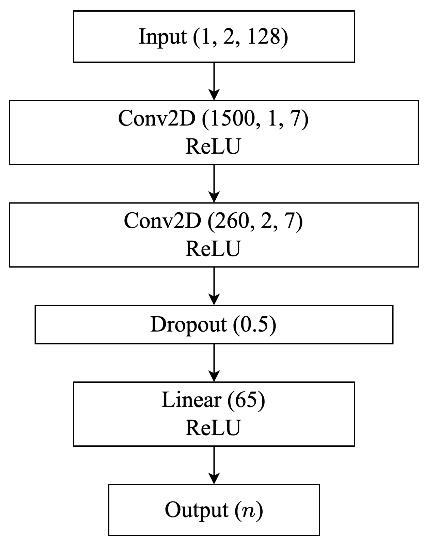
In this work, all synthetic data experiments utilize a single architecture trained across pairwise combinations of source/target datasets with varying (1) SNRs, (2) FOs, (3) SNRs and FO, or (4) modulation types in order to identify the impact of these parameters of interest on TL performance for an AMC use-case. Given the large number of models trained for these experiments, training time was a primary concern when selecting the model architecture. Therefore, the synthetic data experiments use a simple CNN architecture, shown in Figure 5, that is based on the architecture used in [28], with a reduction in the input size. Although many works have found success using larger input sequences [28,38,39], works such as [16,17] have found 128 input samples to be sufficient. Recognizing that longer input sequences result in increased computation and training time, in this work, 128 raw IQ samples are used as input corresponding to approximately 16–32 symbols depending on the symbol rate of the example. These samples are fed to the network in a $(1,2,128)$ tensor, such that 1 refers to the number of channels, 2 refers to the IQ components, and 128 refers to the number of samples. The network contains two 2D convolutional layers; the first uses 1500 kernels of size $(1,7)$ and the second uses 260 kernels of size $(2,7)$. The second convolutional layer is followed by a flattening layer, a dropout layer using a rate of 0.5, and two linear fully connected layers containing 65 and n nodes, where n is the number of output classes (i.e., modulation schemes) being trained. Both convolutional layers and the first linear layer use a ReLU activation function, and the final linear layer uses a Softmax activation function.

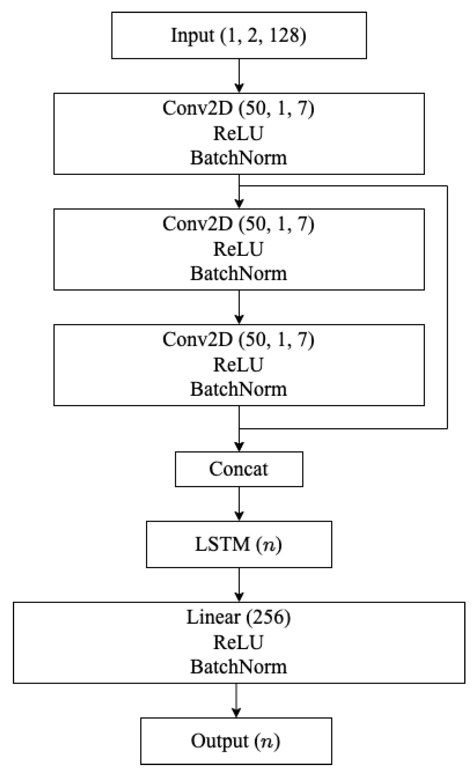
All experiments performed using captured data (both AMC and SEI use-cases) utilize a convolutional long-short term deep neural network (CLDNN) architecture, shown in Figure 6, which represents a more complex architecture than the small and simple CNN used in the synthetic dataset experiments. The CLDNN architecture uses both convolutional and long short-term memory (LSTM) layers, in addition to batch normalization, and could more reasonably be used in real-world systems. In [16], CLDNNs, outperformed baseline CNNs, LSTMs, inception modules, and residual networks for an AMC task, and have since been used to perform AMC throughout the literature [3,40]. In this work, the use of this architecture is extended to the SEI use-case as well.

Again, 128 raw IQ samples (approximately 16 symbols worth of samples) are used as input to the CLDNN architecture, fed to the network in a $(1,2,128)$ tensor. The CLDNN architecture begins with three convolutional layers, each with 50 kernels of size (1, 7) and zero padding to maintain the input size. Each convolutional layer is followed by a ReLU activation function and a batch normalization layer. The outputs of the first and third convolutional block, post batch normalization, are then concatenated along the channel dimension forming a $(100,2,128)$ tensor, reshaped, preserving the time dimension, to form a $(200,128)$ tensor, and passed through a single LSTM layer with n hidden cells, where n is the number of output classes. The output of the LSTM layer is then flattened and passed through a fully connected linear layer with 256 nodes, a ReLU activation function, and a batch normalization layer. Finally, the output layer is fully connected with n nodes with a Softmax activation function.

3.5. Training and Evaluation

For all model architectures, use-cases, and dataset types, the model pre-training and TL process remains the same and is shown in Figure 4b. For pre-training, the training dataset contained 5000 examples per class, and the validation dataset contained 500 examples per class. These dataset sizes, called the “full”-sized data subsets from here on out, are consistent with [28] and adequate to achieve consistent convergence. Each model was trained using the Adam optimizer [41] and Cross Entropy Loss [42], with the PyTorch default hyper-parameters [43] (a learning rate of 0.001, without weight decay), for a total of 100 epochs. A checkpoint was saved after the epoch with the lowest validation loss, and was reloaded at the conclusion of the 100 epochs.

This work examines two popular types of TL methods: head re-training and model fine-tuning. For head re-training and model fine-tuning, “limited”-sized data subsets are used that contain 500 examples per class in the training dataset, representing a smaller sample of available target data. The head re-training and fine-tuning processes both used the Adam optimizer and Cross Entropy Loss as well, with checkpoints saved at the lowest validation loss. During head re-training, only the final layer of the model was trained, again using the PyTorch default hyper-parameters, while the rest of the model’s parameters were frozen. During fine-tuning, the entire model was trained with a learning rate of 0.0001, an order of magnitude smaller than the PyTorch default of 0.001. While a more comprehensive comparison of head re-training and fine-tuning is out of the scope of this work, in general, head re-training is more time-efficient and less computationally expensive than fine-tuning, as there are far fewer trainable parameters. For example, for the CNN and CLDNN architectures used in this work, head re-training requires only 1518 and 5911 trainable parameters in comparison to the 7,434,243 and 796,093 trainable parameters needed for fine-tuning.

For all experiments performed herein, top-1 accuracy is used as the performance metric throughout this work, and is used to compare the performance of different source models transferred to a single target dataset, as well as to the baseline models described above. The performance of the TL models is also compared to baseline models trained on the “limited”-size data subsets. These baseline models have the same CNN and CLDNN architectures as the TL models and were from random initialization using the same training hyper-parameters described for pre-training (the Adam optimizer, Cross Entropy Loss, etc.). Furthermore, when comparing the difference between head re-training, fine-tuning, and the limited-data baseline performance for a single target domain and task, the target dataset is the exact same (same examples) across these three models.

For the experiments performed on the captured dataset, a multinomial-based decision aggregation method [44] is used to integrate decisions on successive examples decisions into a single, generally higher, confidence result using 10 successive examples per AMC decision and 100 successive examples per SEI decision. This aggregation helps mitigate decreases in performance caused by the added complexity of the captured data and makes the performance trends more clear across the parameters of interest. The SEI use-case required more successive examples per aggregated decision because the distinguishing features for SEI are smaller variations in the raw IQ, compared to AMC, that become more apparent over longer durations. The addition of the multinomial-based decision aggregation scheme does not presume unreasonable amounts of data per decision: approximately 160–320 symbols worth of data for the AMC use-case and approximately 1600 symbols worth of data for the SEI use-case. Given that the data were captured at a 250 kHz sample rate and 8 samples per symbol, this corresponds to only 0.005–0.01 s worth of capture per AMC decision or 0.05 s worth of capture per SEI decision.

3.6. Experiments

3.6.1. Synthetic Data Domain Adaptation Experiments

The examination of RF domain adaptation performance begins with experiments using synthetically generated datasets and an AMC use-case. The synthetic dataset used in this work and described previously was created to contain an even distribution of reasonable SNRs and FOs. Then, subsets of the data were selected according to various parameters of interest, artificially creating different domains. Source models were pre-trained on each domain and then transferred to the remaining domains in the experiment using both head re-training and model fine-tuning. Using this approach, performance is examined as a function of SNR alone, FO alone, and SNR and FO jointly, addressing each of the domain adaptation settings in Section 2.2—environment adaptation, platform adaptation, and environment platform co-adaptation. Sweeps over these three parameters of interest resulted in the training and evaluation of 4524 models over 81 data subsets, corresponding to approximately 2588 h and 50 min of training time.

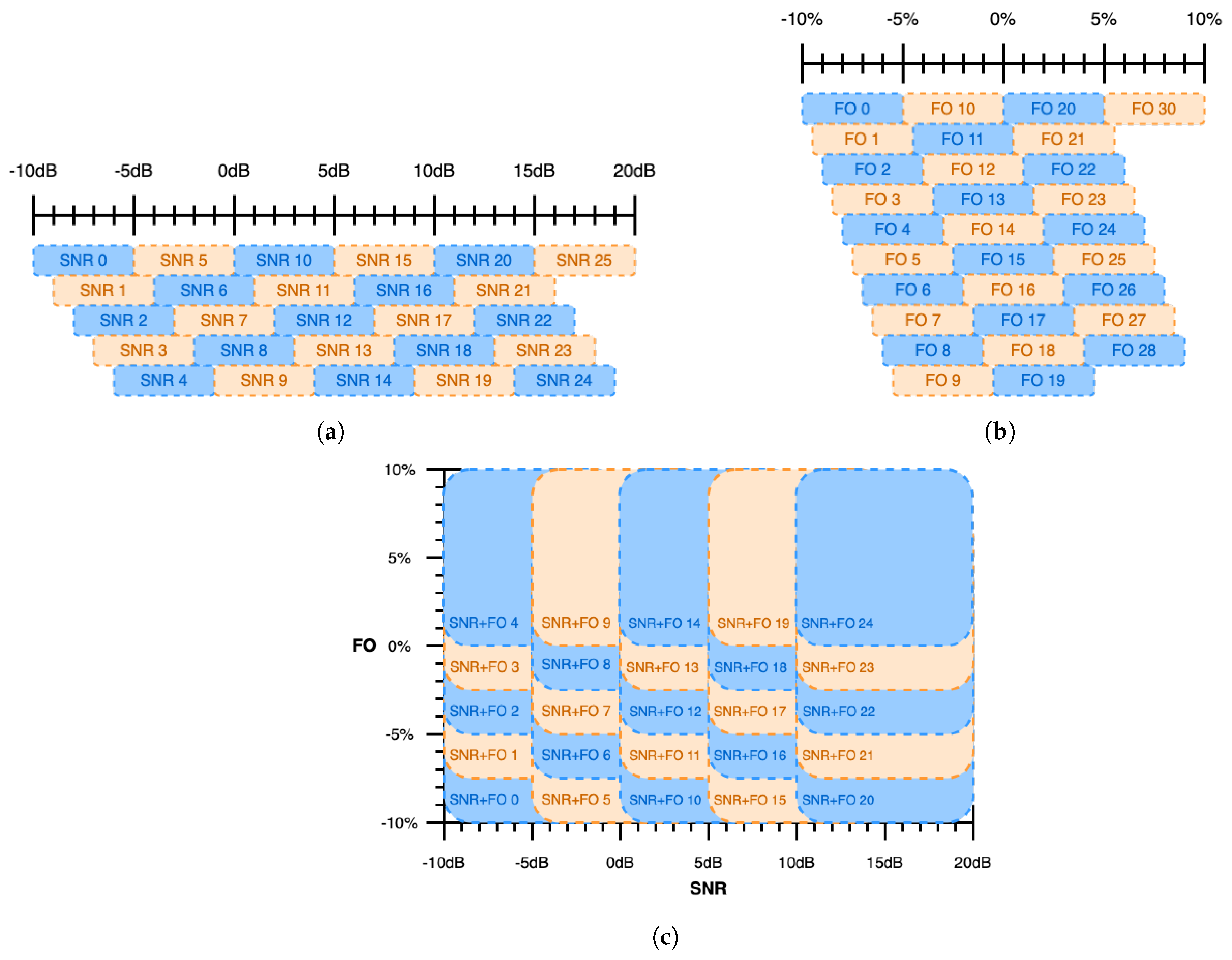
The sweep over SNR represents an environment adaptation problem, characterized by a change in the RF channel environment such as an increase/decrease in the additive interference, $\nu \left[t\right]$, of the channel and/or transmitting devices such as an increase/decrease in the magnitude, $\alpha \left[t\right]$, of the transmitted signal. For this experiment, 26 source data subsets were constructed from the synthetic master dataset containing examples with SNRs selected uniformly at random from a 5 dB range sweeping from −10 dB to 20 dB in 1 dB steps (i.e., [−10 dB, −5 dB], [−9 dB, −4 dB], ..., [15 dB, 20 dB]), as shown in Figure 7a. FO was selected uniformly at random in the range [−5%, 5%] of sample rate. This SNR sweep yielded 26 baseline models and 26 pre-trained source models, each of which was transferred to the remaining 25 target data subsets, for a total of 650 models transferred using head re-training and 650 models transferred using fine-tuning.

The sweep over FO represents a platform adaptation problem, characterized by a change in the Tx and/or Rx devices such as an increase/decrease in ${\omega }_{\Delta }\left[t\right]$ due to hardware imperfections or a lack of synchronization. For this experiment, 31 source data subsets were constructed from the synthetic master dataset containing examples with FOs selected uniformly at random from a 5% range sweeping from −10% of sample rate to 10% of sample rate in 0.5% steps (i.e., [−10%, −5%], [−9.5%, −4.5%], ..., [5%, 10%]), as shown in Figure 7b. SNR was selected uniformly at random in the range [0 dB, 20 dB]. This FO sweep yielded 31 baseline models and 31 pre-trained source models, each of which was transferred to the remaining 30 target data subsets, for a total of 930 models transferred using head re-training and 930 models transferred using fine-tuning.

The sweep over both SNR and FO represents an environment platform co-adaptation problem, characterized by a change in both the RF channel environment and Tx/Rx devices. For this experiment, 25 source data subsets were constructed from the synthetic master dataset containing examples with SNRs selected uniformly at random from a 10 dB range sweeping from −10 dB to 20 dB in 5 dB steps (i.e., [−10 dB, 0 dB], [−5 dB, 5 dB], ..., [10 dB, 20 dB]) and with FOs selected uniformly at random from a 10% range sweeping from −10% of sample rate to 10% of sample rate in 2.5% steps (i.e., [−10%, 0%], [−7.5%, 2.5%], ..., [0%, 10%]), as shown in Figure 7c. This SNR and FO sweep yielded 25 baseline models and 25 pre-trained source models, each of which was transferred to the remaining 24 target data subsets, for a total of 600 models transferred using head re-training and 600 models transferred using fine-tuning.

3.6.2. Captured Data Domain Adaptation Experiments

The results of these initial experiments on synthetic data are then verified and extended using captured data, an additional neural network (NN) architecture, and both AMC and SEI use-cases. More specifically, to examine how the Rx, propagation environment, and CF independently and jointly impact RF TL behavior, 27 data subsets are constructed, each captured using different Rxs, Rx locations, and/or CFs, holding only the Tx hardware constant. The impacts of the propagation environment alone on RF TL performance are identified by examining performance across changes in Rx location (creating different channels) while holding Tx and Rx hardware and CF constant. As previously discussed, three different Rx locations are present in the master captured dataset: an in-room line-of-sight location, an in-room partial occlusion location, and an adjacent room location. The impacts of CF alone on RF TL performance are identified by examining performance across changes in CFs while holding the Tx and Rx hardware and Rx location constant. Three different CFs are present in the master captured dataset: 346.3 MHz, 416.4 MHz, and 783.4 MHz. The impacts of the Rx hardware alone on RF TL performance are identified by examining performance across changes in Rx hardware, while holding the Tx hardware, CF, and Rx location constant. Three different collection nodes are used in the construction of the master captured dataset; two host USRP B200s, and the third hosts a USRP E310. The impacts of propagation environment, CF, and Rx hardware, together, on RF TL performance are identified by examining performance across changes in all three of these parameters. These experiments are performed for both the AMC and SEI use-cases, resulting in the training of 54 baseline models, 54 pre-trained source models, 1404 head-retrained models, and 1404 fine-tuned models for each use-case.

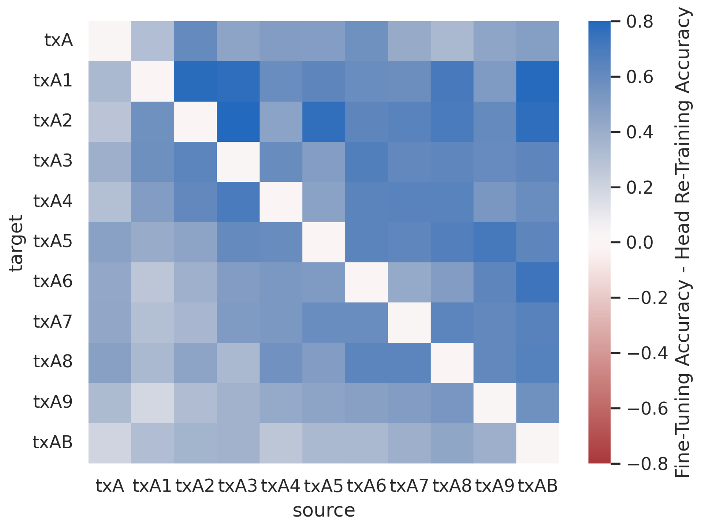
Additionally, the impact of the Tx hardware on RF TL performance is isolated by creating 4 data subsets from the captured master dataset, each transmitted by either Tx Group A, Tx Group B, Tx Group C, or All Tx, where Tx Groups A/B/C each contain 10 Txs randomly selected without replacement. For this experiment, all Txs are co-located, and the Rx hardware, Rx location, and CF are constant between data subsets, using only collection node 1 (hosting a USRP B200) at the in-room partial occlusion location capturing at 346.3 MHz. This experiment is performed for the AMC use-case only, as changing the Tx hardware in an SEI setting would change the task. Therefore, experiments examining the impact of Tx hardware on RF TL performance in an SEI setting are discussed in the next chapter on Sequential Learning. Having already trained baseline and source models for the All Tx setting during the previous experiment, this experiment resulted in the training of three additional baseline models, 3 additional pre-trained source models, 12 head re-trained models, and 12 fine-tuned models.

In total, the captured domain adaptation experiments required an additional 857 h of training time.

3.6.3. Synthetic Data Sequential Learning Experiments

As in the domain adaptation experiments, sequential learning performance is first examined using synthetic data for an AMC use-case, then using captured data for both AMC and SEI use-cases. Two experiments are performed using the synthetic dataset: The first experiment aims to investigate TL performance across broad categories of modulation types, namely linear, frequency-shifted, and analog modulation schemes. More specifically, 5 source data subsets were constructed from the larger master dataset containing the modulation schemes shown in Figure 8. For each data subset in this experiment, called “Synthetic Sequential AMC”, SNR was selected uniformly at random in the range [0 dB, 20 dB] and FO was selected uniformly at random in the range [−5%, 5%] of the sample rate. This experiment yielded 5 pre-trained source models, each of which was transferred to the remaining 4 target data subsets, yielding 20 models transferred using head re-training and 20 models transferred using fine-tuning. Additionally, 5 baseline models were trained.

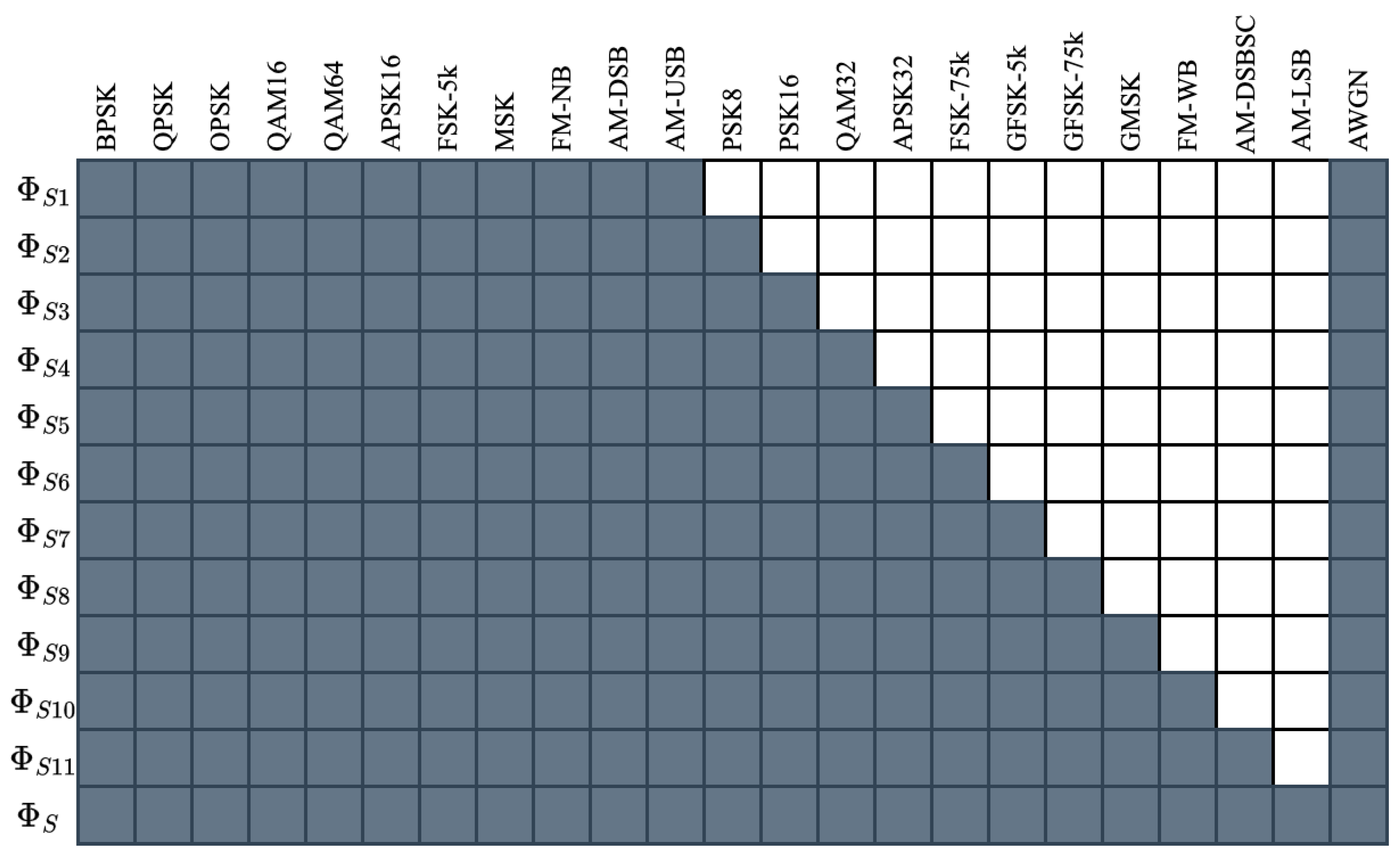
The second experiment performed using synthetic data examines TL performance when a single modulation scheme was added or removed from the source task, or a model refinement scenario. More specifically, the 12 source data subsets were constructed from the larger master dataset containing the modulation schemes shown in Figure 9. Again, SNR was selected uniformly at random in the range [0 dB, 20 dB] and FO was selected uniformly at random in the range [−5%, 5%] of the sample rate. This experiment is called “Synthetic Model Refinement AMC” herein. This experiment yielded 12 pre-trained source models, each of which was transferred to the remaining 11 target data subsets, yielding 132 models transferred using head re-training and 132 models transferred using fine-tuning. Additionally, 12 baseline models were trained.

3.6.4. Captured Data Sequential Learning Experiments

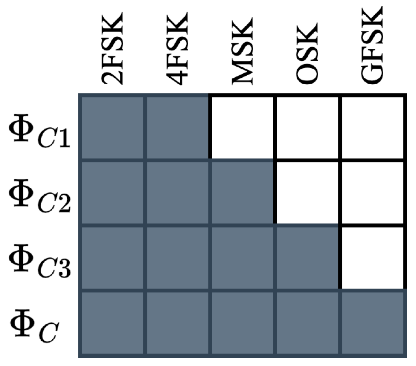
Three additional sequential learning experiments are performed using the captured dataset. For the AMC use-case, only the model refinement experiment is conducted because of the limited number of modulation schemes available. The 4 source data subsets constructed contain the modulation schemes shown in Figure 10. For this experiment, called “Captured Model Refinement AMC”, the Tx and Rx hardware, Rx locations, and CF, were held constant. Four baseline models, 4 pre-trained source models, 12 head-retrained models, and 12 fine-tuned models were trained.

For the SEI use-case, an additional two experiments are conducted mirroring those conducted with the synthetic dataset. The first experiment aims to investigate TL performance across 3 non-overlapping sets of emitters (Tx Group A, Tx Group B, Tx Group C), as well as to the full set of available Tx. For this experiment, called “Captured Sequential SEI”, 4 baseline models, 4 pre-trained source models, 12 head-retrained models, and 12 fine-tuned models were trained. The second experiment examines TL performance when 1–10 Txs are added or removed from the source task, or a model refinement scenario. For this experiment, called “Captured Model Refinement SEI”, 11 baseline models, 11 pre-trained source models, 110 head-retrained models, and 110 fine-tuned models.) For each of these experiments, the Rx hardware, Rx locations, and CF, were held constant.

4. Experimental Results and Analysis

The product of the experiments performed herein is that 5118 models were trained over 81 different domains and 43 different tasks. Given the careful curation of the signal parameters contained within each data subset, the breadth of signal types and parameters observed, and experimentation over both synthetic and real data, AMC and SEI use-cases, and two different NN architectures, generalized conclusions can be drawn regarding TL performance as a function of changes in the propagation environment, Tx/Rx hardware, and task. The following subsections present the results obtained from the experiments performed and discuss insights and practical takeaways that can be gleaned from the results given. Given the large number of experiments performed, representative examples are shown throughout the following subsections.

4.1. Head Re-Training vs. Fine-Tuning

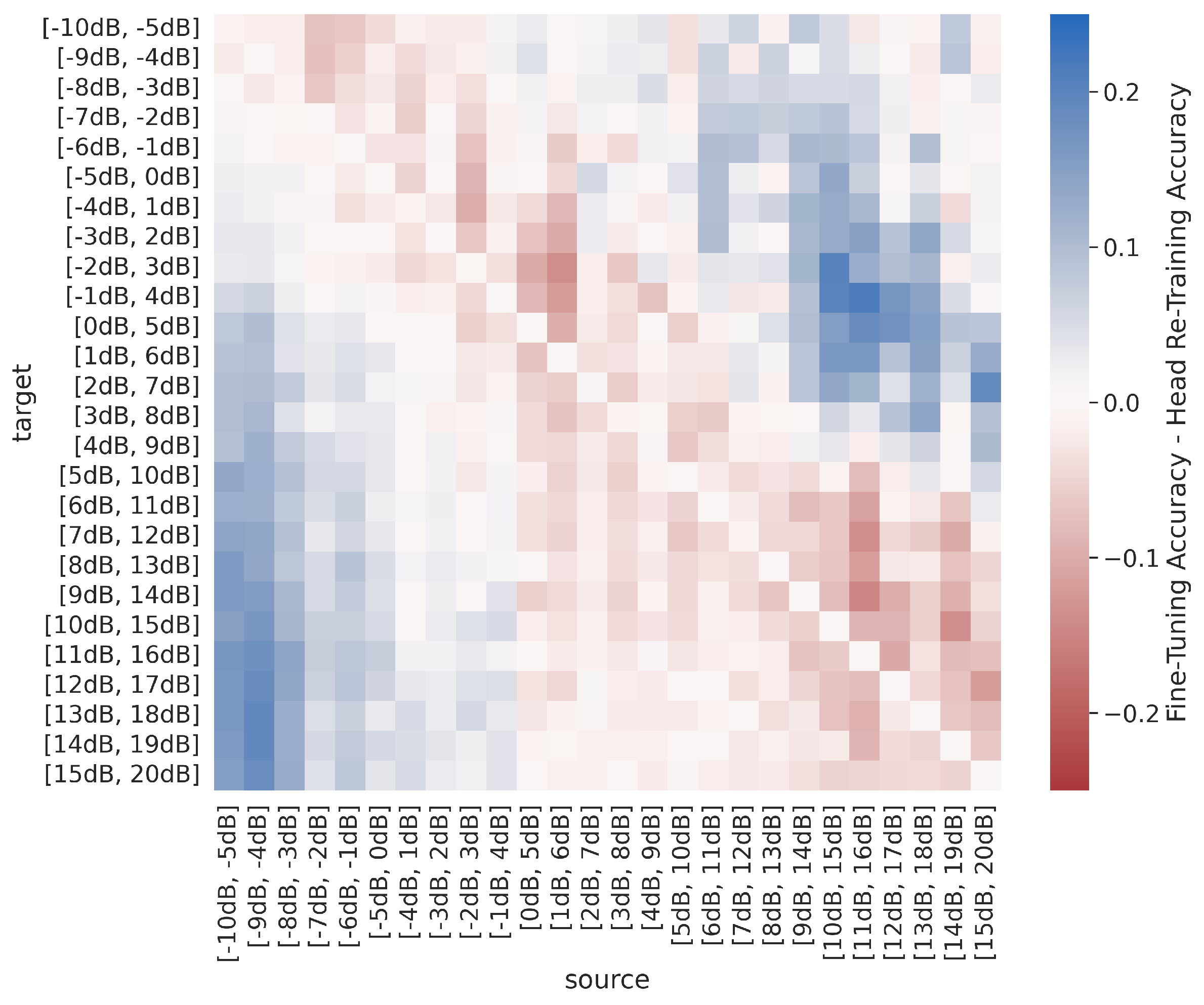
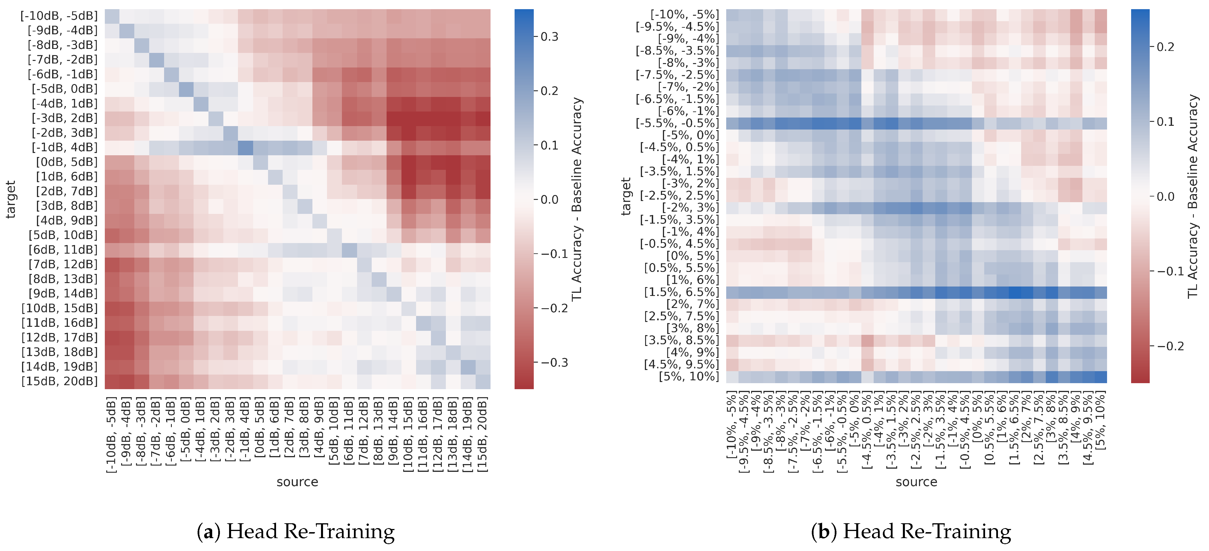
Before examining TL performance in comparison to the baselines in the following subsections, Figure 11 and Figure 12 plot the difference between post-transfer top-1 accuracy achieved using head re-training and fine-tuning such that positive values (in blue) correspond to better fine-tuning performance and negative values (in red) correspond to better head re-training performance for the synthetic sweep across SNR and the captured sequential SEI experiments. Across both the synthetic and captured dataset experiments, results show that when performing domain adaptation, head re-training is as effective, if not more effective, than fine-tuning when TL outperforms the limited-data baseline. In other words, the trend in Figure 11 is very similar to those seen in Figure 13a, discussed further below. Given that head re-training is more time efficient and less computationally expensive than fine-tuning, there is a strong case for using head re-training over fine-tuning when performing RF domain adaptation.

However, when performing sequential learning, fine-tuning generally outperforms head re-training, as shown in Figure 12. Intuitively, these results show that during sequential learning, modifications are needed to the earlier feature learning layers of the model, in order to yield the best performance. Meanwhile, during domain adaptation, we can get away with only modifying the decision-making layer at the end of the model and using the same features learned in the source domain during pre-training.

Also of note, the margins between head re-training and fine-tuning performance are greater in the captured data experiments than in the synthetic data experiments. The synthetic data are observed in a pristine environment compared to the effects of a real-world channel, and as a result, there is far more variance between examples with the “same” metadata parameters in the captured dataset compared to the synthetic dataset. This, in turn, affects not only the complexity of the task, making AMC and SEI more challenging in the real world, but also likely affects the similarity of the source/target datasets. In other words, results thus far have shown that in settings where the source and target domain and/or task are less similar, fine-tuning outperforms head re-training, while head re-training is typically sufficient in settings where the source and target domain and/or task are similar.

Given these results, in the remaining results subsections, only head re-training results will be shown for the domain adaptation experiments and only fine-tuning results will be shown for the sequential learning experiments.

4.2. Synthetic Domain Adaptation Experiments

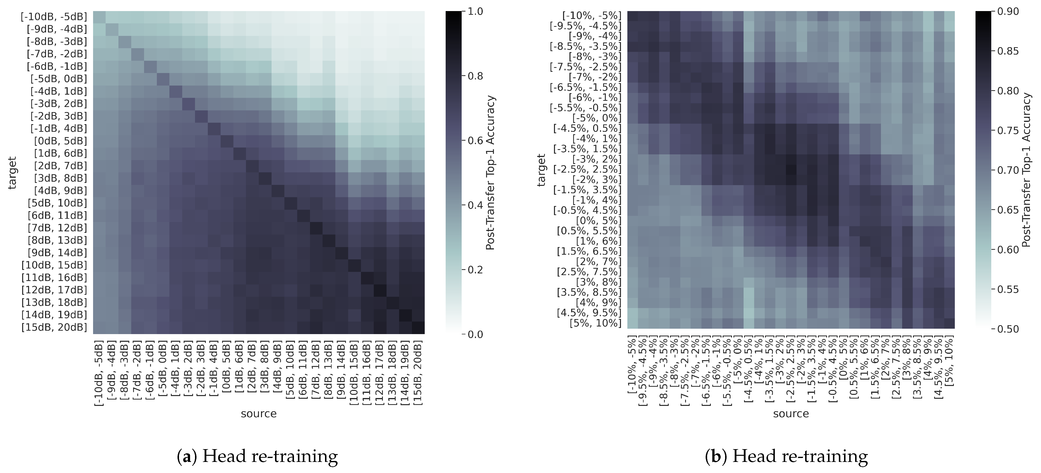
The heatmaps in Figure 14 show the post-transfer top-1 accuracy achieved with each of the synthetic source/target dataset pairs for the sweeps across SNR alone and FO alone. Results indicate that highest post-transfer performance is achieved when the source and target domains are most similar, along the diagonal of the heatmap, as all other metadata parameters are held constant. These trends are expected, as models trained on similar domains likely learn similar features, and is consistent with the general theory of TL [18], as well as existing works in modalities outside of RF [45].

Figure 14 also shows that transfer across changes in FO is approximately symmetric, while transfer across changes in SNR is not. This behavior can be attributed to changes in the relative “difficulty” between the source and target domains. More specifically, changing the source/target SNR inherently changes the difficulty of the problem, as performing AMC in lower SNR channel environments is more challenging than performing AMC in high SNR channel environments. Therefore, the post-transfer accuracies achieved in the lower SNR target domains are lower overall than the post-transfer accuracies achieved in the higher SNR target domains. In contrast, changing the source/target FO does not make performing AMC any more or less difficult but may require modifications to the learned features to accommodate. This can be likened to performing FO calibration, as is standard practice in Rx operations. Consequently, small changes in FO, ${\omega }_{\Delta }\left[t\right]$, in either the positive or negative direction, are expected to perform similarly. Figure 14b indeed shows that TL performance is approximately symmetric, with the best performance closest to the diagonal where the source and target FO ranges are most closely aligned.

However, it is important to note that a comparatively lower post-transfer accuracy does not necessarily correspond to a failed transfer, as post-transfer accuracy is also impacted by the difficulty of the target domain. In other words, transferring from an “easier” domain to a “harder” domain may result in a net loss of performance in terms of post-transfer top-1 accuracy, but TL may still outperform the limited-data baseline. Figure 13 presents the difference between post-transfer top-1 accuracy and target limited-data baseline accuracy for the SNR and FO sweeps, such that when the difference value is positive the TL model outperforms the baseline model and vice versa. These results show that for the sweep over SNR, the TL model only outperforms the baseline near the diagonal where the source and target are very similar, including when transferring between the lowest SNR ranges. However, for the sweep over FO, the TL model outperforms the baseline for a greater number of source/target pairs. Also notable, while the TL performance across SNR is not symmetric, as shown in Figure 14a, Figure 13a shows that the relative performance of the TL models to the baseline models is not significantly impacted by SNR. Additionally, there appear to be some target domains where all source models transfer well, as indicated by the horizontal blue bands. The cause of this trend is not readily apparent and may be explored in follow on research.

Practically, these trends suggest that the effectiveness of RF domain adaptation increases as the source and target domains become more and more similar, and, when applicable, RF domain adaptation is more often successful when transferring from harder to easier domains when compared to transferring from easier to harder domains. For example, transferring from [−5 dB, 0 dB] to [0 dB, 5 dB] SNR is likely more effective than transferring from [5 dB, 10 dB] to [0 dB, 5 dB] SNR. Although the distance between source/target datasets (as measured by the relative change in SNR) in these two transfer scenarios is the same, the SNR increases from source to target in the first case and decreases from source to target in the second case. However, transferring from a FO range of [−9%, −4%] of the sample rate to [−8%, −3%] of the sample rate is likely more effective than transferring from a FO range of [−10%, −5%] of the sample rate to [−8%, −3%] of the sample rate, as the distance between source/target datasets (as measured by the relative change in FO) is greater in the second case.

In the settings where the domains are sufficiently dissimilar, Figure 13 shows that better performance is achieved via training from random initialization on the limited-sized target training dataset rather than from using TL. This result can be explained by the much lower learning rate used during TL in these experiments compared to the baseline models. More specifically, while the lower learning rate used during TL helps to combat overfitting, models will not converge/overfit as much as the baseline models in the same number of training iterations. Increasing the learning rate during TL would likely mitigate this discrepancy between TL and baseline model performance, and is left for future work.

Recalling that the sweep over SNR can be regarded as an environment adaptation experiment and the sweep over FO can be regarded as a platform adaptation experiment, the results of these synthetic dataset experiments suggest that changes in channel environment are more challenging to overcome using TL techniques than changes in Tx/Rx hardware, such that environment adaptation is more difficult to achieve than platform adaptation. More specifically, if the source/target SNR ranges do not overlap to some degree, better performance is achieved through simply training from random initialization on the target data, even if there is a limited amount of labeled target data available. However, for overcoming changes in FO, TL is generally more successful than the limited-data baseline, especially when using model fine-tuning.

4.3. Captured Domain Adaptation Experiments

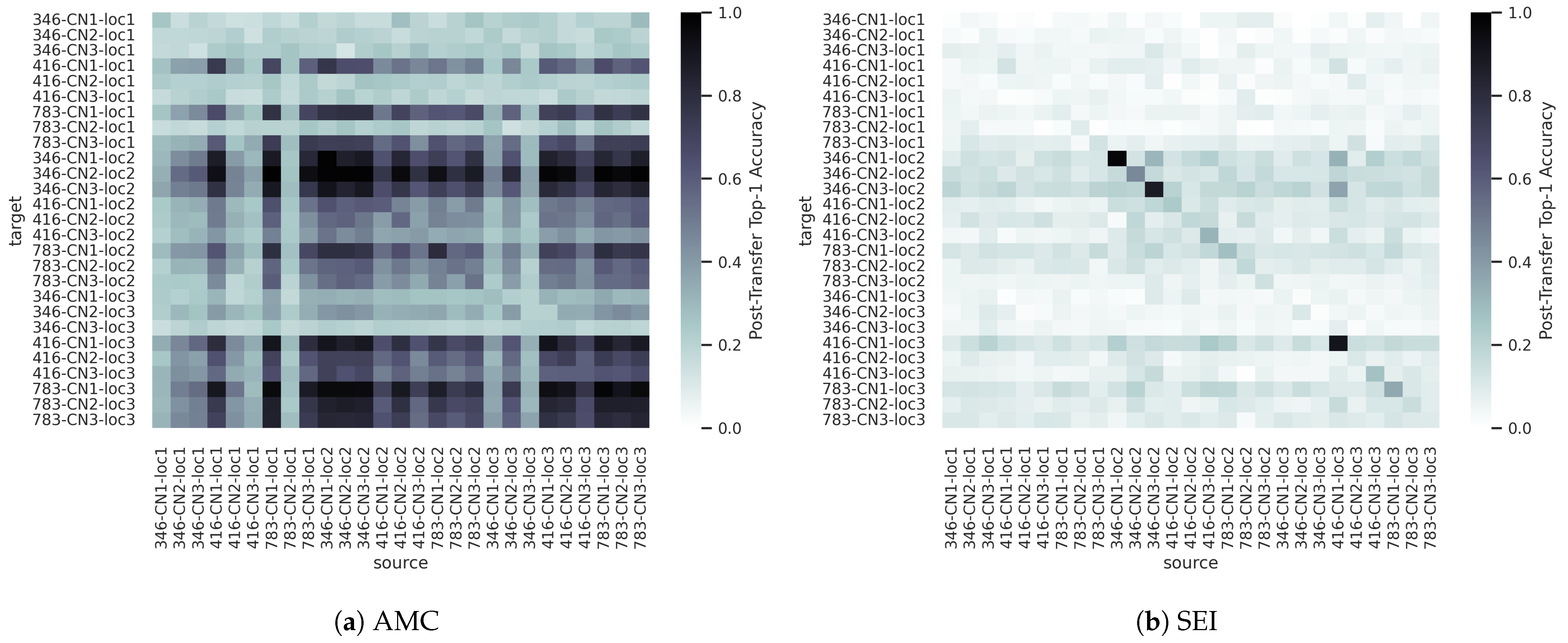
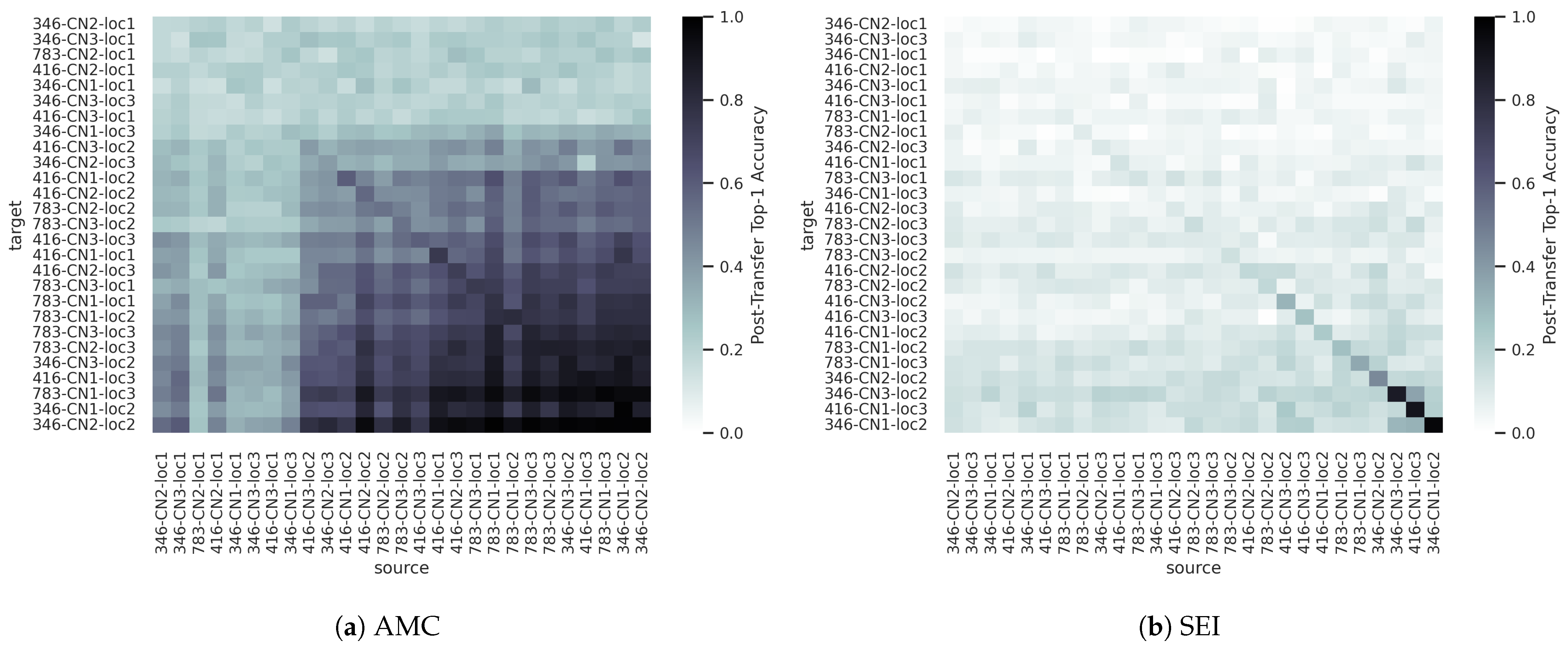
The heatmaps in Figure 15 shows the post-transfer top-1 accuracy achieved with each of the captured source/target dataset pairs for the AMC and SEI use-cases. While the synthetic dataset experiments provided results with clear and straightforward trends, the added complexity and real-world effects present in the captured dataset make deciphering the trends in Figure 15 more challenging. Notably, TL performance does not seem to be dictated by CF, Rx ID, or Rx location individually, and baseline performance varies significantly from domain to domain. That is, some domains are more “difficult” than others, similar to the synthetic sweep over SNR discussed previously.

Taking this into consideration, Figure 16 shows the same post-transfer top-1 accuracy values of Figure 15, but with the rows and columns sorted in order of the limited-data baseline accuracy, with the lowest baseline accuracy on the upper/left and the highest baseline accuracy on the bottom/right. The simple act of sorting by baseline accuracy yields clearer trends in the data very similar to that seen in the synthetic sweep over SNR (Figure 14a), seemingly according to some notion of domain “difficulty”. More specifically, accuracy generally increases as one moves down and/or to the right in the plot, but not according to specific CFs, Rx IDs, or Rx locations, in particular. Again, all source models appear to transfer a select few of the target domains, as indicated by the horizontal blue bands. 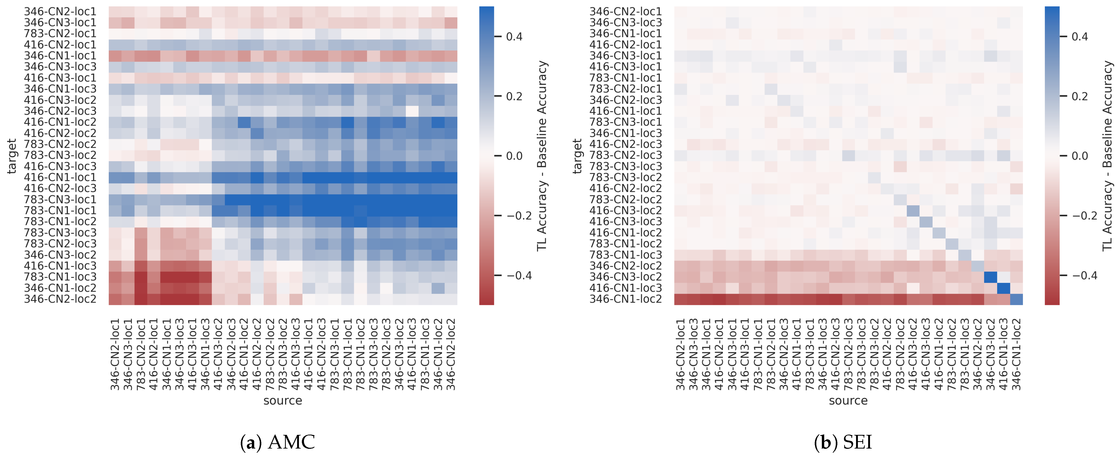Unlike for the synthetic dataset experiments, however, Figure 17 shows that for the captured dataset AMC experiments, TL outperforms the limited-data baseline in most settings.

Given these results, the primary question is the cause of the relative differences in domain “difficulty”. While the synthetic dataset experiments isolated one parameter of interest and completely controlled for all other variables, the domains created in the captured dataset experiment are composed of three different parameters (CF, Rx ID, and Rx location), each of which directly or indirectly impact values such as carrier/center frequency offset (CFO), signal/noise power, and SNR. The results in Figure 16 and Figure 17 suggest that neither CF, Rx ID, or Rx location independently encourages or prevents transfer to other CFs, Rx IDs, or Rx locations, as there are no apparent trends associated with any one CF, Rx ID, or Rx location in particular. 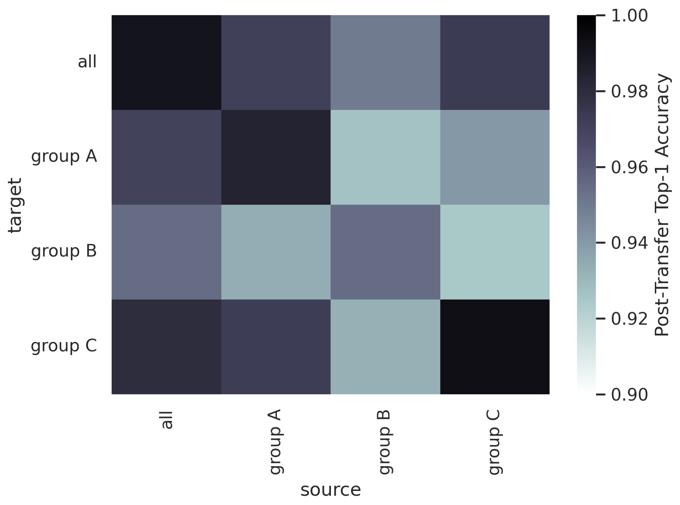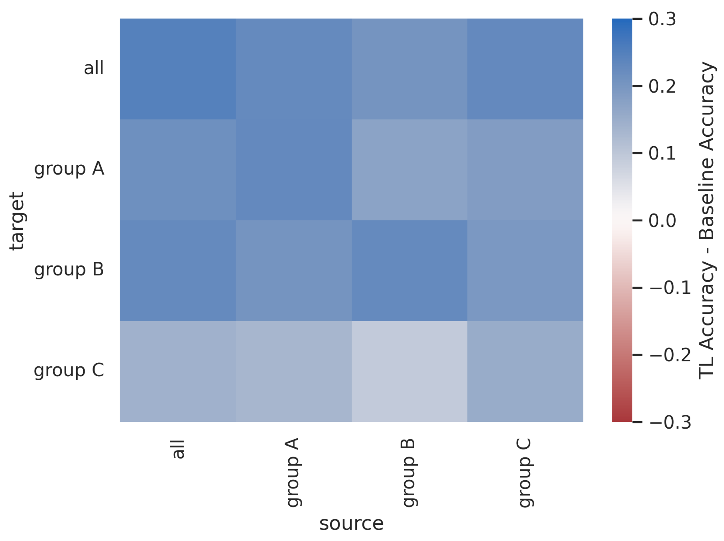Similarly, Figure 18 and Figure 19 show that changes in groups of Tx alone also do not have a significant impact on TL performance of the AMC use-case. While there is some slight variation in performance across the Tx groups, post-transfer accuracy is consistently high and transfer is good between all source/target pairs, always outperforming the limited-data baseline.

TL performance is seemingly better predicted by the relative performance of the source and target baseline models, with transfer more likely to occur when the source baseline model outperforms the target baseline model. Given that CFO is corrected before training and does not appear to be statistically different between domains, the most apparent hypothesis for the cause of the relative performance differences between domains is a change in SNR, though is almost certainly not the sole contributor. 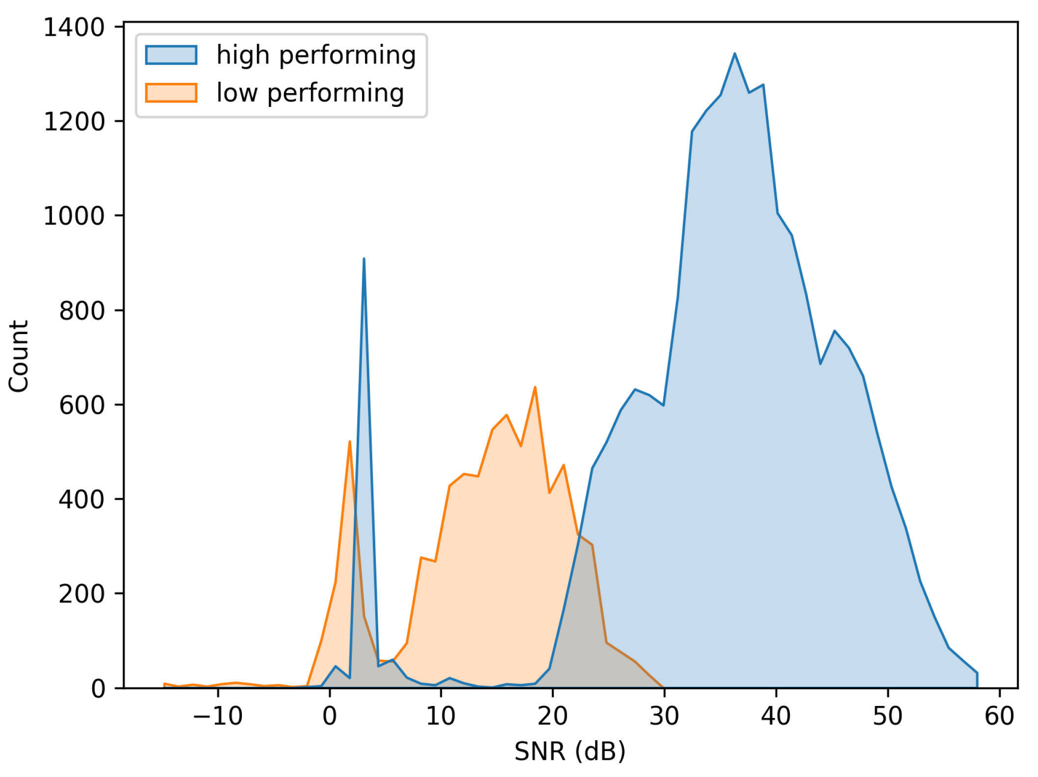Figure 20 shows the distribution of SNRs for all data points in the bottom three performing domains and the top three performing domains. On average, the data points from the higher performing domains have an approximately 20 dB higher SNR than those from the lower performing domains. However, the SNR of all data points in the captured dataset is sufficiently high that a decrease of 10 dB SNR should not result in such severe performance degradations.

A secondary hypothesis is that performing TL using a larger target dataset size (i.e., 20–50% of the source dataset size) might minimize the relative performance differences between domains, effectively smoothing out the post-transfer top-1 accuracy plots in Figure 15 and Figure 16. If this were the case, it may indicate that despite using three different Rx locations, the SNRs in each channel created are not sufficiently different and/or low enough to yield the performance trends seen in the synthetic dataset experiments across SNR. Although this work has focused on varying only the parameters within the RF data while fixing the TL methods, follow-up work could address this question by (1) experimenting with RF data captured in a wider variety of conditions and (2) experimenting with larger amounts of data.

Experimentation with larger datasets would also likely improve the results of the SEI experiments. In comparison to the AMC use-case, post-transfer accuracy is lower in the SEI use-case, as a result of the more challenging task and increased number of output classes, TL outperforms the limited-data baseline less frequently and to a far lesser degree. Despite this, the performance trends remain the same between the AMC and SEI use-cases. Increasing the source and/or target dataset sizes, and potentially introducing further regularization or learning rate scheduling could improve the performance of the SEI approach and should be investigated in future work.

4.4. Sequential Learning across Signal Types

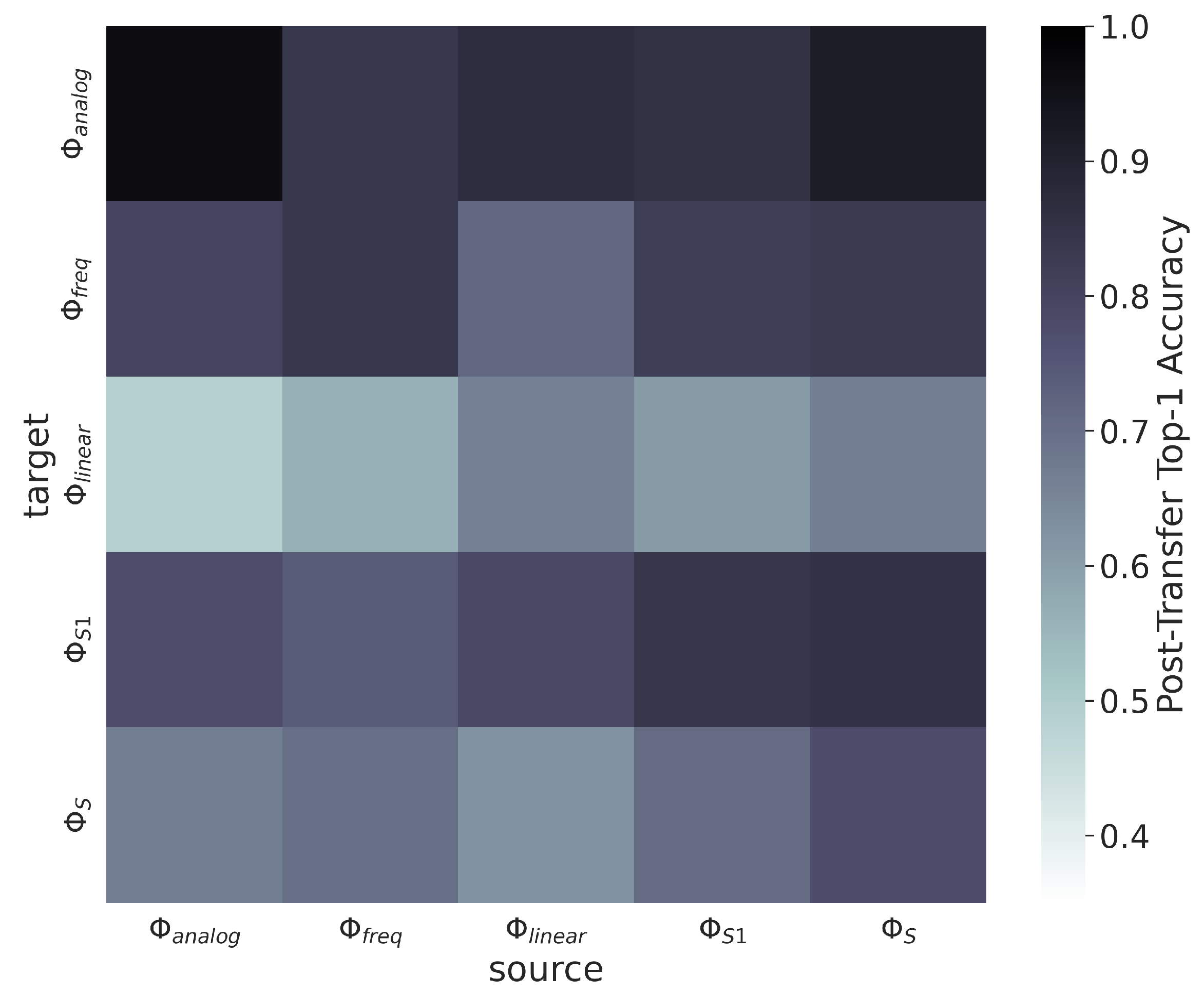
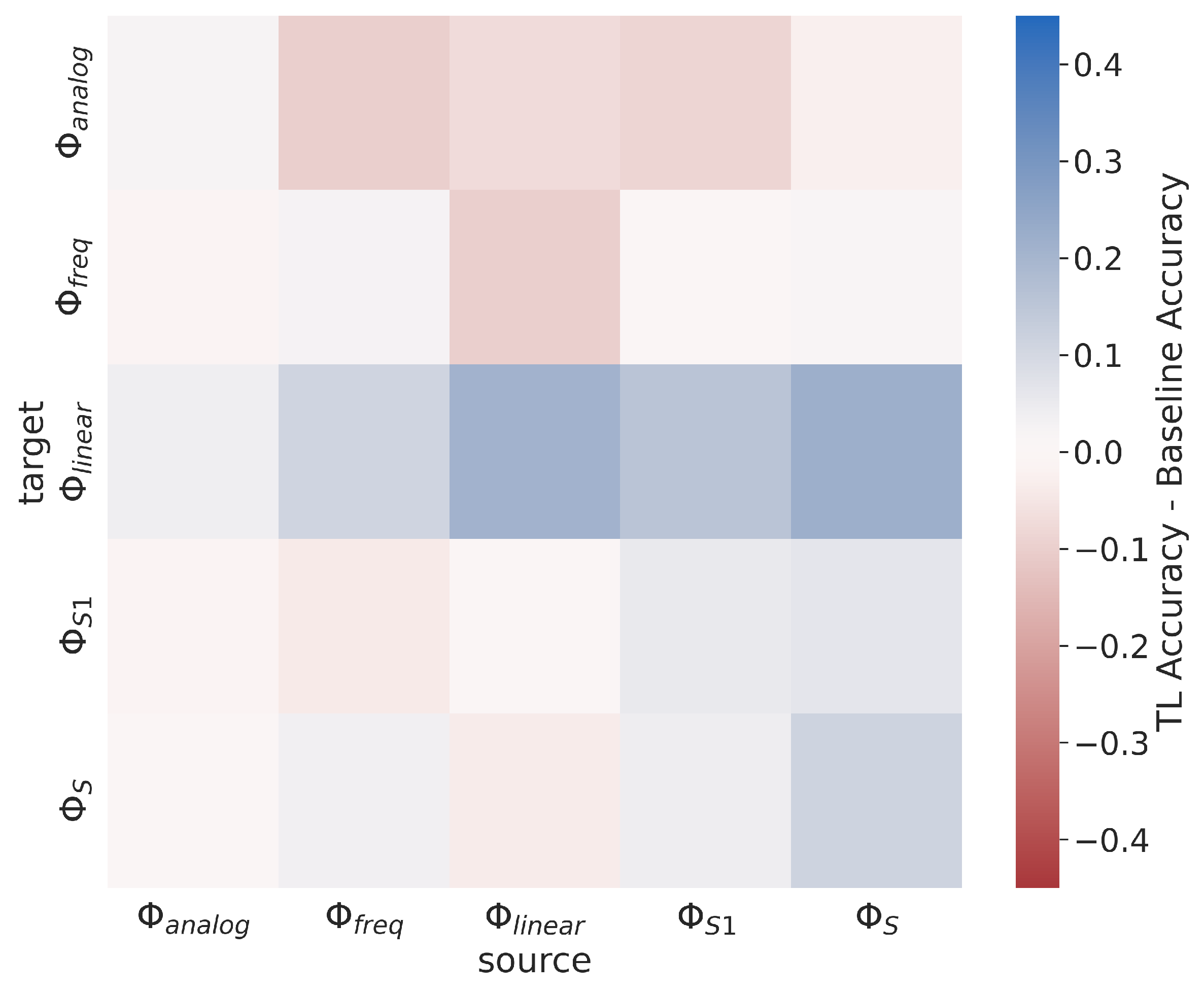
Figure 21 shows the post-transfer top-1 accuracy for each source/target dataset in the Synthetic Sequential AMC experiment. Results indicate that the subsets containing only a single type of modulation scheme (the analog, frequency-shifted, and linear subsets) do not transfer well between one another, and also do not transfer well to the subsets which contain multiple types of modulation schemes (the small and all subsets). Meanwhile, the small and all subsets transfer fairly well to the analog, frequency-shifted, and linear subsets. These results are verified by the results shown in Figure 22 which presents the difference between post-transfer top-1 accuracy and the limited-data baseline target models, and shows that TL only increases performance over the baseline models when there is significant overlap between the modulation schemes in each subset.

These results are expected considering the general setting in which TL is beneficial: when the source and target are “similar”. When there are no similar signal types between source/target, there is little to no benefit to using TL, such as when attempting transfer between the analog, frequency-shifted, and linear subsets. However, because the small and all subsets contain at least one modulation scheme from each of the analog, frequency-shifted, and linear subsets, the pre-trained source model has some prior knowledge of each category of modulation schemes from which to build. Practically, these results indicate that for this AMC use-case, TL is only beneficial when similar signal types are present in the source and target datasets.

4.5. Sequential Learning across Groups of Txs

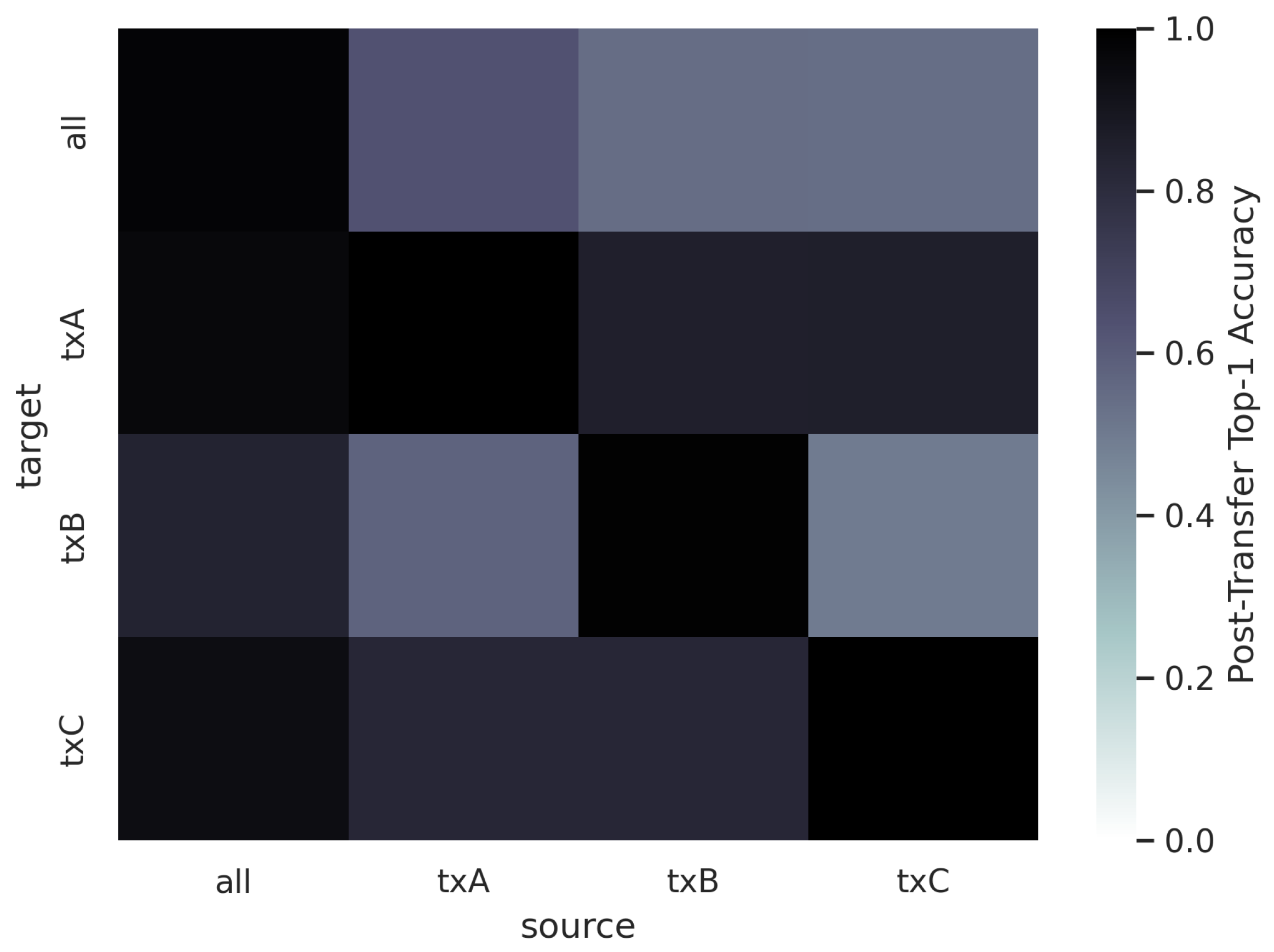
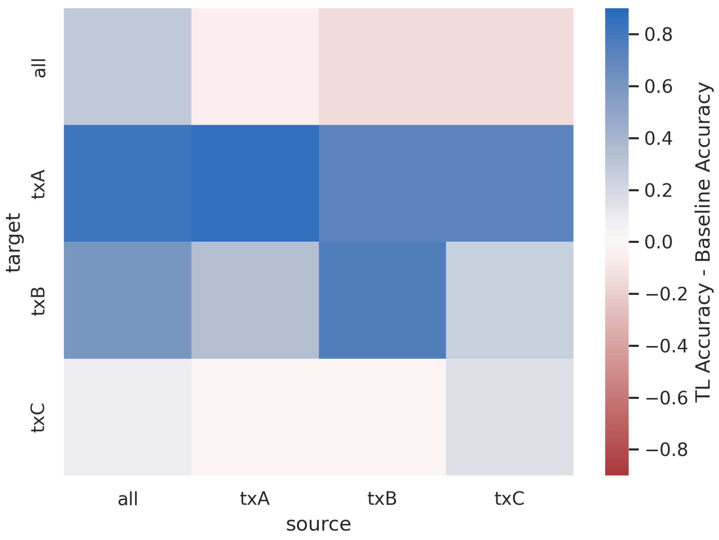
Figure 23 and Figure 24 show the post-transfer top-1 accuracy and the difference between post-transfer top-1 accuracy and target limited-data baseline accuracy for each source/target dataset in the Captured Sequential SEI experiment. Note that the increases in performance when the source and target are the same (i.e., along the diagonal) are due to the 10x increase in training data between the baseline and pre-trained models. Figure 23 and Figure 24 indicate that the model trained on all Txs transfers well to the non-overlapping Tx groups A, B, and C. This trend is similar to that shown for the Synthetic Sequential AMC experiment (Figure 21). The model trained on all Txs has prior knowledge about each of the groups A, B, and C because Tx groups A, B, and C are each subsets of all Txs. Interestingly, all of the sub-groups transfer well to Tx groups A and B, but none of them transfer particularly well to Tx group C. This further reinforces the concept that TL behavior is not symmetrical (i.e., txC transfers to txA, but txA does not transfer to txC). This would also suggest that the Txs in groups A and B are more similar to one another than the Txs in group C, despite the fact that every Txs in this dataset is of the same make and model.

4.6. Sequential Learning for Successive Model Refinement

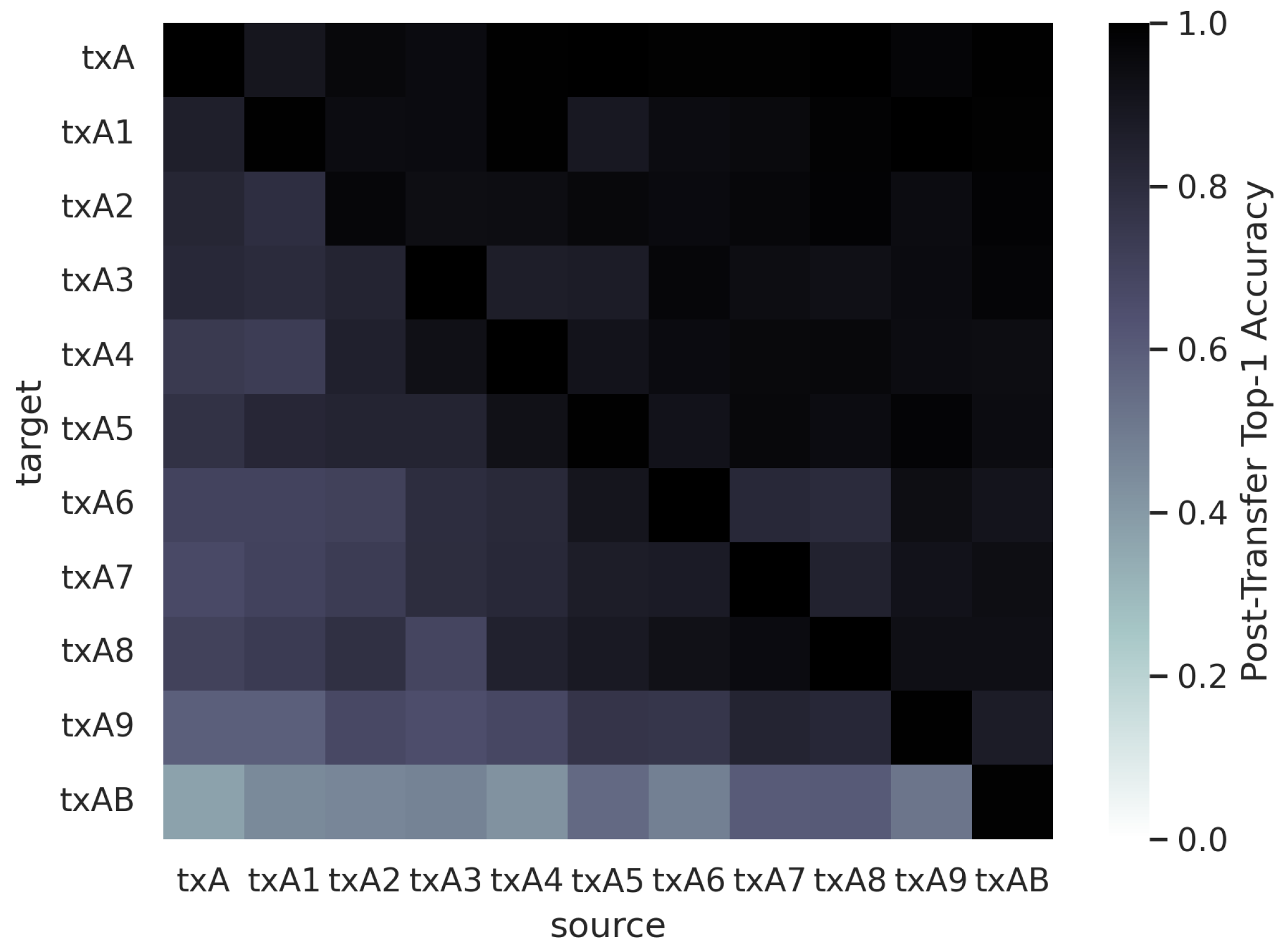
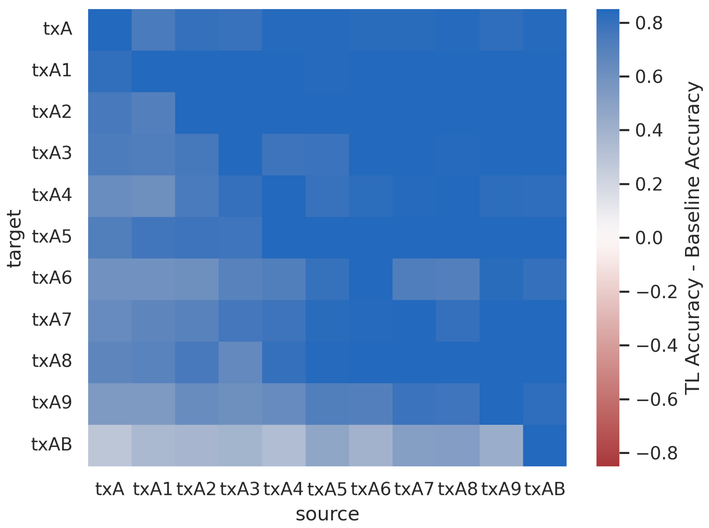
Across all model refinement experiments, results indicate that it is easier to remove output classes during TL than it is to add output classes. This trend is particularly evident in Figure 25 and Figure 26, which present the post-transfer top-1 accuracy and the difference between the post-transfer top-1 accuracy and target limited-data baseline accuracy for the Captured Model Refinement SEI experiment. More specifically, performance is highest in the upper triangle of the heatmaps in Figure 25 and Figure 26, indicating not only the best overall TL performance, but the most significant performance benefits over the target baseline models. Again, the increase in performance along the diagonal of the heatmaps in Figure 25 and Figure 26 is due to the 10x increase in training data between the baseline and pre-trained models.

This behavior is consistent with results given in [22] and intuitive, as it is easier to forget or disregard prior knowledge than to acquire new knowledge during transfer. More specifically, by pre-training on a larger subset of signal types or Tx IDs, the source model has already learned features to identify all of the modulation classes or Txs in the target task. In fact, the source model has likely learned more features than necessary to perform the target task and could undergo feature pruning in order to reduce computational complexity. It should also be noted that the task becomes easier as output classes are removed, further contributing to the trend. Practically, these results dictate that one should utilize a source task that encompasses the target task, when possible.

5. Conclusions and Future Work

TL is a pervasive technology in CV and NLP, yielding significant performance improvements in settings with limited training data, as well as reduced training time, by leveraging prior knowledge gained from data with different distributions. However, while recent works seek to mature ML and DL techniques in applications related to wireless communications, few have demonstrated the use of TL techniques for yielding performance gains, improved generalization, or to address concerns of training data costs. Designing TL algorithms for the RFML space first requires a fundamental understanding of how the RF domain and RF tasks impact learned behavior and inhibit or facilitate transfer. Even for RFML works that have successfully used TL, such limits in understanding may hinder further performance improvements that might be yielded from TL techniques. Additionally, these limitations in understanding also obscure insights into long-term model behavior during deployment, which has long been a criticism of RFML and prevented commercial support and deployment [2].

To begin to address this deficit, this work systematically evaluated RF TL performance across changes in channel type, SNR, CF, FO, transmitter/receiver hardware, and modulation type for AMC and SEI use-cases using three different NN architectures. Through this exhaustive study, a number of guidelines have been identified for when and how to use RF TL successfully. More specifically, results indicate that when only limited amounts of target training data are available, TL almost always achieves better performance over training from random initialization, in terms of accuracy, time, and computational complexity, but more research is needed to confirm this trend. In the experiments over synthetic datasets, TL only provided top-1 accuracy improvements over the limited-data baselines when the source and target domains and tasks are “similar”. However, in the captured dataset experiments, TL outperforms the limited-data baseline, in terms of accuracy, in most settings. Given that the captured dataset is more representative of what would be encountered by a real-world system, as well as the time and computational complexity benefits of using TL versus training from random initialization, these early results support the use of TL in most settings where representative training data are limited.

Additionally, when performing domain adaptation it is important to consider domain difficulty, as well as domain similarity. Additional research is needed to understand the origins of domain difficulty and discussed further in the next subsection, but when one domain is more difficult than the other, TL performance is better when transferring from the harder domain to the easier domain. What is well understood from the results presented in this work is that the channel, and subsequent impact on SNR, is a contributing factor to domain difficulty, and must be considered when attempting to perform RF TL, as it has a significant impact on performance. Meanwhile, FO and Tx/Rx hardware impact RF TL performance to a much lesser degree. In other words, environment adaptation and environment platform co-adaptation are far more challenging than platform adaption.

When performing sequential learning over changes in a task, it is beneficial for there to be some overlap between the source and target task, such that the intersection between the source task outputs and target task outputs is non-empty, the source task is a subset of the target task, or vice versa. The best sequential learning performance is achieved when the target task is a subset of the source task. For example, when performing model refinement, results showed better performance when removing output classes than when adding output classes. This guideline can be attributed to the fact that (1) the target task becomes easier as output classes are removed and (2) the model does not need to do any significant feature learning from the target data. Instead, the task is simplified, and any unnecessary features learned previously can eliminated.

Finally, while further research is needed to better understand how to best perform RF TL, the results presented herein have shown the relative benefits of using head re-training versus fine-tuning. More specifically, when performing domain adaptation, head-retraining generally performed as well, if not better than, fine-tuning, and when performing sequential learning across changes in the task model fine-tuning vastly outperformed head re-training. Depending on the size of the model and the computational resources available, model fine-tuning may be quite a bit more expensive than head re-training, both computationally and in terms of training time. For the CNN and CLDNN model architectures used in this work, using head re-training versus fine-tuning resulted in an overall reduction of 99.98% and 99.27% in trainable parameters, respectively.

These initial guidelines are subject to further experimentation using additional signal types, channel models, use-cases, model architectures, and datasets. Continuing and extending the analysis conducted herein will provide a more thorough understanding of RF TL behavior and performance across a wider range of use-cases and deployment settings. Additional suggested directions for experimentation include the following:

• Analysis of multi-task learning behavior using synthetic and captured data. While work in [46] showed a proof-of-concept approach for performing multi-task AMC and SEI using a combination DenseNet and Transformer network architecture, and showed improved performance over single-task models, the approach has yet to be evaluated on captured data or across changes in domain and task.
• Analyses of TL performance for other RFML use-cases, such as signal detection and spectrum anomaly detection, and additional model architectures, such as Transformer-based or generative network architectures.
• Analysis of RF TL performance across changes in both domain and task or simultaneous domain adaptation and sequential learning.
• An analysis of RF TL techniques for transferring between use-cases. For example, examining transfer between AMC and SEI use-cases.
• Analysis of RF TL performance across synthetic, augmented, and captured datasets. Work in [3] has shown that training RFML models on synthetic data alone does not yield sufficient performance on captured, real-world data for deployment. However, intelligently augmenting the data to match the SNR, FO, and sample rate mismatch to the deployed environment can greatly improve performance on the captured data. If small amounts of labeled captured data are available for training, TL provides an approach to further improve the performance of models pre-trained on synthetic or augmented data in real-world settings.

Additionally, the results of the domain adaptation experiments performed herein showed that TL performance was not solely predicted by metadata parameters such as CF, Rx ID, or channel, but was correlated with baseline performance or domain difficulty. This has raised the following question: what dictates domain difficulty? While SNR is a clearly contributing factor to domain difficulty, it does not seem to be the only factor. To address this question more fully, experiments including more CF, Rx ID, and channel variations and varying additional parameters of interest, such as fading/multi-path channel environments, sample rate, and temperature would provide greater context and more data points from which to derive performance trends, and cleaner, more controlled captured datasets, perhaps collected in an anechoic chamber, together with data augmentation, would provide more granular variation in domain and yield smoother trends.

Finally, this work has focused on how changes in the RF domain and task impact TL performance, keeping the TL methods fixed. Future research should address the counter side of this work by examining RF TL performance as a function of various TL hyperparameters and training schemes, while generalizing over the source and target domains and tasks, including the following:

• Using unsupervised, self-supervised, semi-supervised, or weakly supervised pre-training methods;
• Varying learning rate and/or using learning rate schedulers;
• Varying source and target dataset size;
• Varying the number of layers frozen and/or fine-tuned;
• Using fine-tuning methods such as chain thaw [47] or gradual/scheduled unfreezing [48,49].

Provided future verification and refinement of these results and guidelines, these guidelines can be used in future RFML systems to construct the highest performing models for a given target domain when data are limited. More specifically, these guidelines begin a discussion regarding how best to continually update RFML models once deployed, in an online or incremental fashion, to overcome the highly fluid nature of modern communication systems [2]. However, additional work is needed to develop the framework for using TL techniques in real-world systems, including methods and metrics for source model selection or estimating model transferability and for initiating RF TL. Several modality-agnostic source model selection and transferability metrics already exist in the literature and could be applied to the RFML systems, such as Log Expected Empirical Prediction (LEEP) [50], Logarithm of Maximum Evidence (LogME) [51], Optimal Transport-based Conditional Entropy (OTCE) [52], TransRate [53], and Gaussian Bhattacharyya Coefficient (GBC) [54]. Promising methods for initiating RF TL include those used to identify dataset drift or covariance shift [55], methods for detecting out-of-distribution examples [56,57], as well as uncertainty quantification methods such as temperature scaling [58] or Bayesian approximation [59]. Such methods are not only required for initiating TL, but also help provide user-assured performance, and are important for ruggedizing the decision chain against spoofing and other adversarial techniques.