
Locally-Scaled Kernels and Confidence Voting


Abstract
1. Introduction
2. Background

3. The Similarity Kernel
3.1. Theoretical Framework—Preserving the Topology
- It is assumed the data points are distributed uniformly on a Riemannian manifold embedded in the vector space . This manifold represents the underlying natural structure of the data.
- 2.
- If g is locally constant in an open neighborhood U, then within a ball with radius r of volume centered at point the geodesic distance from to any point is where d is the Euclidean distance in . This is because the geodesic distance in the neighborhood is bound by the Euclidean distance on the tangent plane at .
- 3.
- A simplex is a generalized triangle. From algebraic topology, it is known that a simplicial approximation of a manifold can be used to capture the topological aspects of that manifold [32].
- 4.
- Similarity is a symmetric property.
3.2. The Locally Scaled Symmetric Laplacian Diffusion Kernel
3.3. Kernel Computational Complexity
4. Applications of Kernels in Classification
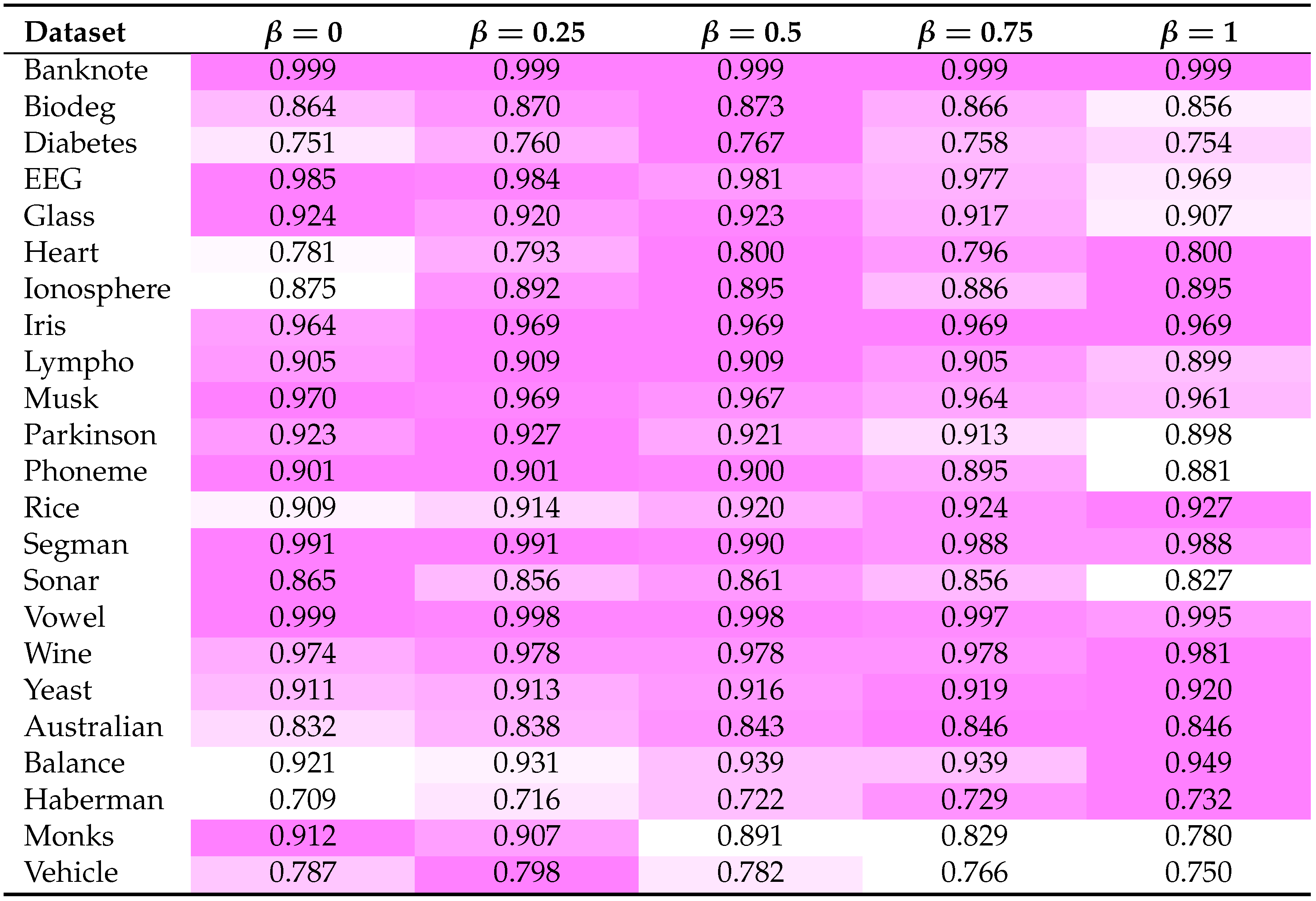
4.1. Confidence Voting and the Blended-Model
4.2. Regularization
4.3. Classification Computational Complexity
5. Evaluation Methods
5.1. Datasets
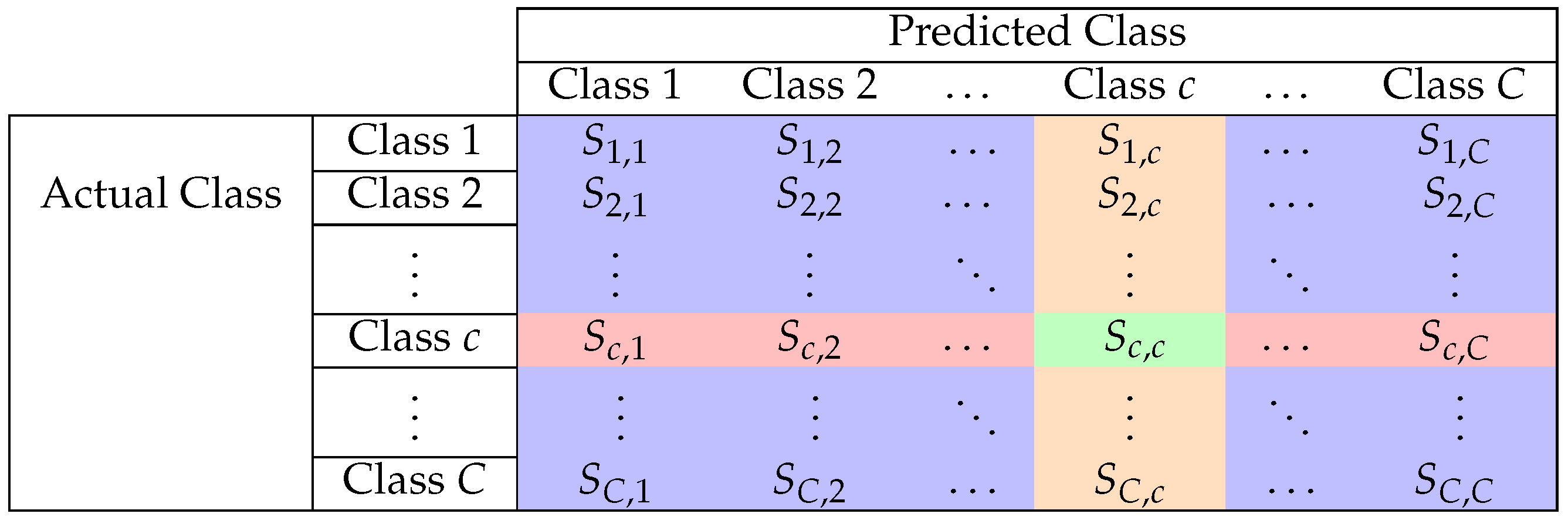
5.2. Accuracy
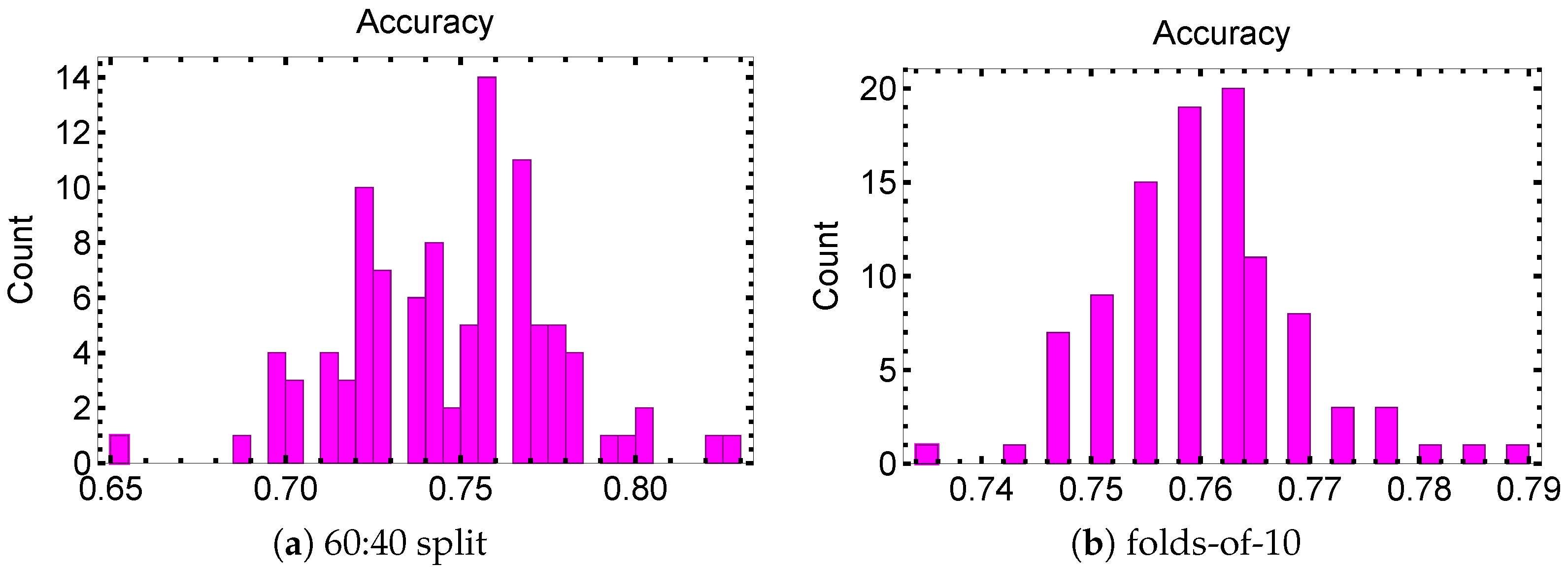
5.3. Train–Test Split
5.4. Pre-Processing
6. Experimental Results
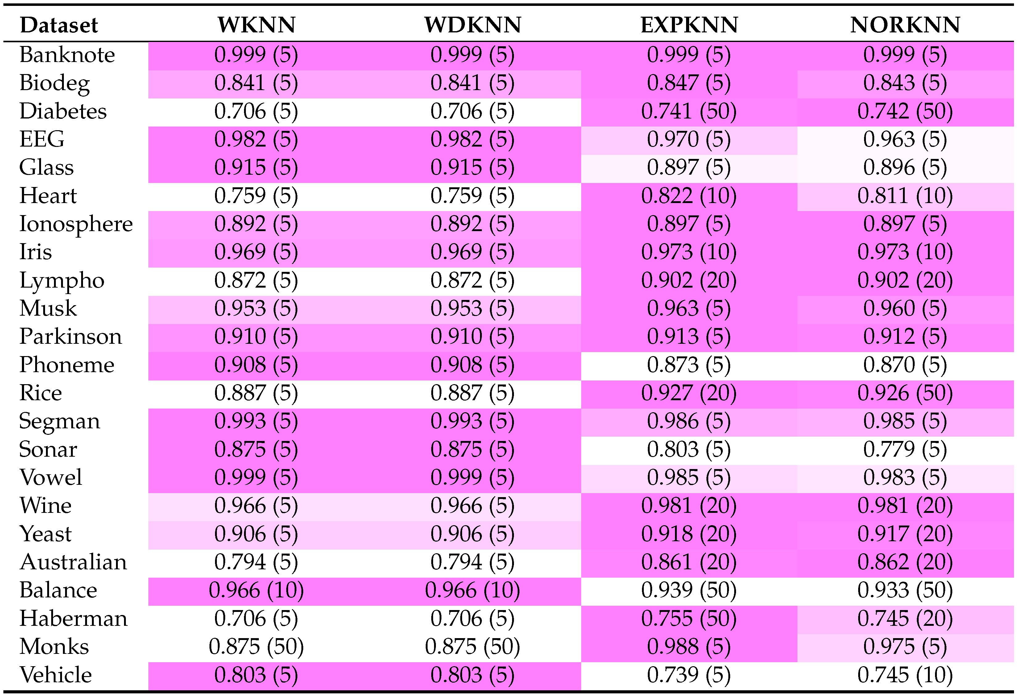
6.1. Baselines
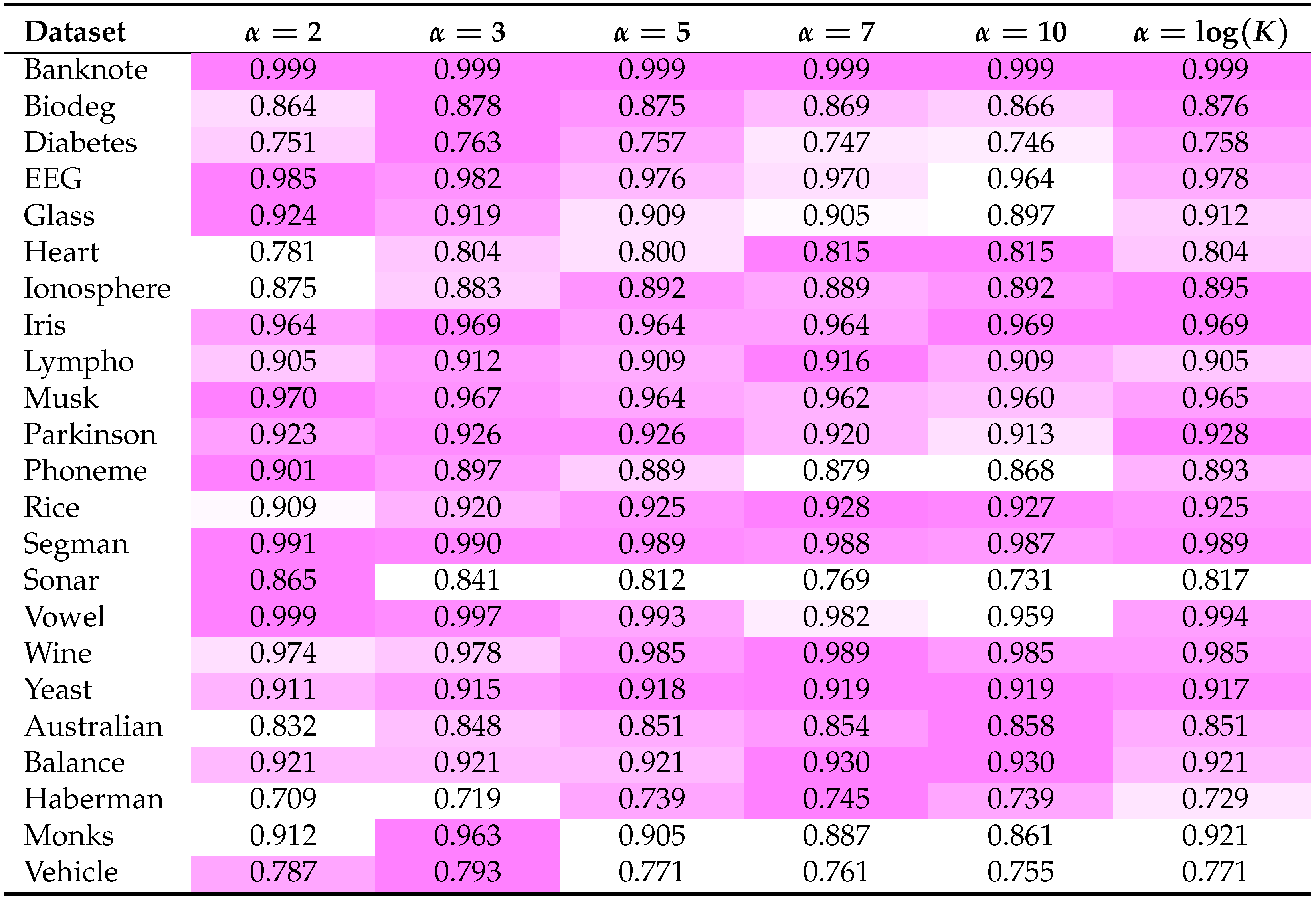
6.2. One Tuning for All
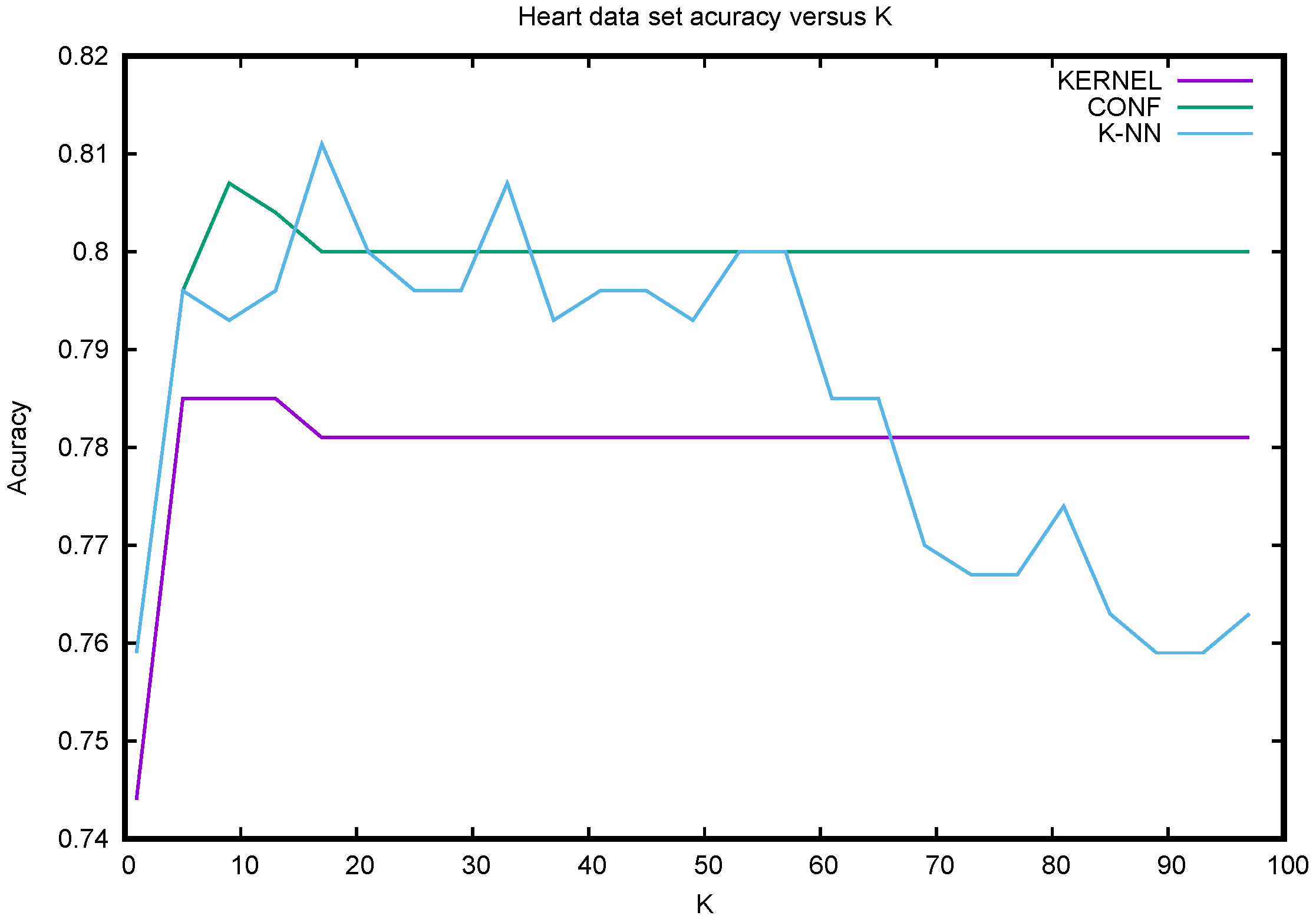
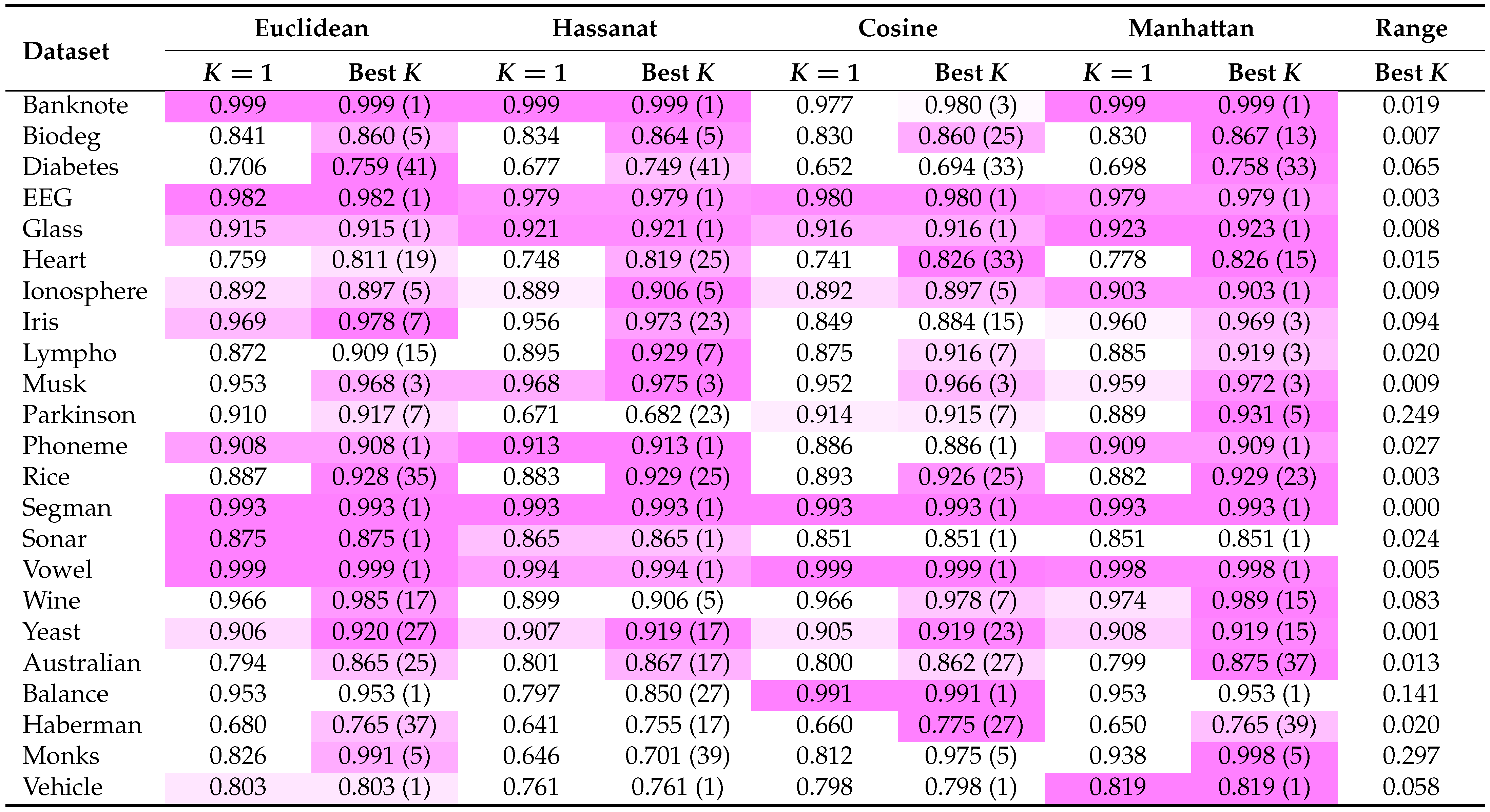
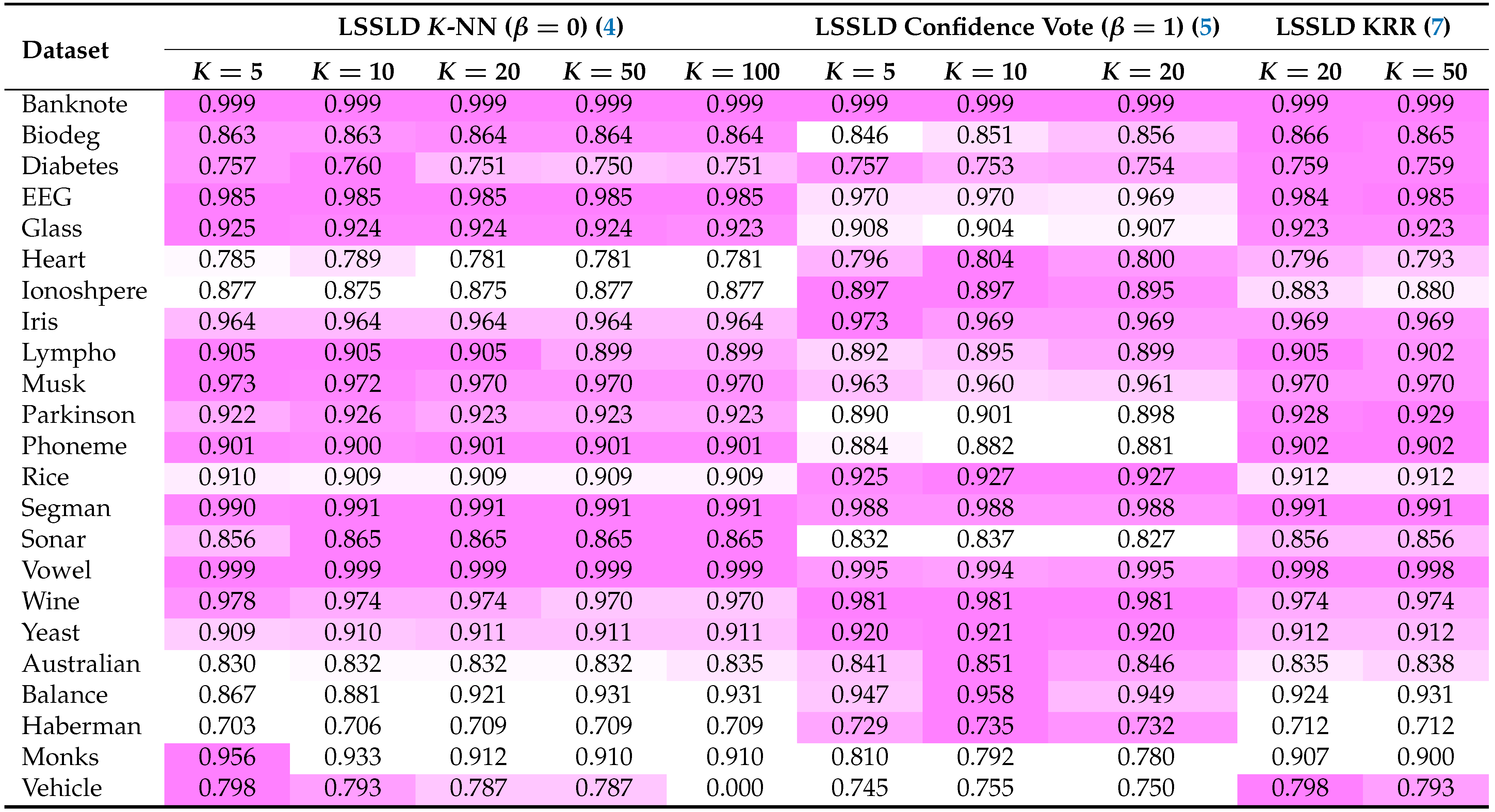
6.3. LSSLD Kernel Comparison
7. Conclusions
8. Future Work
Author Contributions
Funding
Data Availability Statement
Conflicts of Interest
Abbreviations
| DRT | Dimensionality Reduction Techniques |
| DWKNN | Distance Weighted K-Nearest Neighbors |
| EXPKNN | Exponentially weighted K-Nearest Neighbors |
| KRR | Kernel Ridge Regression |
| LSSLD | Locally Scaled Symmetric Laplacian Diffusion |
| K-NN | K-Nearest Neighbors |
| NORKNN | Normally weighted K-Nearest Neighbors |
| SVM | Support Vector Machine |
| t-SNE | t-distributed Stochastic Neighbor Embedding |
| UCI | University of California Irvine |
| UMAP | Uniform Manifold Approximation and Projection |
References
- Abu Alfeilat, H.A.; Hassanat, A.B.; Lasassmeh, O.; Tarawneh, A.S.; Alhasanat, M.B.; Eyal Salman, H.S.; Prasath, V.S. Effects of distance measure choice on k-nearest neighbor classifier performance: A review. Big Data 2019, 7, 221–248. [Google Scholar] [CrossRef]
- Alkasassbeh, M.; Altarawneh, G.A.; Hassanat, A. On enhancing the performance of nearest neighbour classifiers using hassanat distance metric. arXiv 2015, arXiv:1501.00687. [Google Scholar]
- Nayak, S.; Bhat, M.; Reddy, N.S.; Rao, B.A. Study of distance metrics on k-nearest neighbor algorithm for star categorization. J. Phys. Conf. Ser. 2022, 2161, 012004. [Google Scholar] [CrossRef]
- Zhang, C.; Zhong, P.; Liu, M.; Song, Q.; Liang, Z.; Wang, X. Hybrid metric k-nearest neighbor algorithm and applications. Math. Probl. Eng. 2022, 2022, 8212546. [Google Scholar] [CrossRef]
- Yean, C.W.; Khairunizam, W.; Omar, M.I.; Murugappan, M.; Zheng, B.S.; Bakar, S.A.; Razlan, Z.M.; Ibrahim, Z. Analysis of the distance metrics of KNN classifier for EEG signal in stroke patients. In Proceedings of the 2018 International Conference on Computational Approach in Smart Systems Design and Applications (ICASSDA), Kuching, Malaysia, 15–17 August 2018; IEEE: Piscataway, NJ, USA, 2018; pp. 1–4. [Google Scholar]
- Ratnasari, D. Comparison of Performance of Four Distance Metric Algorithms in K-Nearest Neighbor Method on Diabetes Patient Data. Indones. J. Data Sci. 2023, 4, 97–108. [Google Scholar] [CrossRef]
- Hofer, E.; v. Mohrenschildt, M. Model-Free Data Mining of Families of Rotating Machinery. Appl. Sci. 2022, 12, 3178. [Google Scholar] [CrossRef]
- Ghojogh, B.; Ghodsi, A.; Karray, F.; Crowley, M. Reproducing Kernel Hilbert Space, Mercer’s Theorem, Eigenfunctions, Nyström Method, and Use of Kernels in Machine Learning: Tutorial and Survey. arXiv 2021, arXiv:2106.08443. [Google Scholar]
- Kang, Z.; Peng, C.; Cheng, Q. Kernel-driven similarity learning. Neurocomputing 2017, 267, 210–219. [Google Scholar] [CrossRef]
- Rousseeuw, P.J.; Hubert, M. Robust statistics for outlier detection. In Wiley Interdisciplinary Reviews: Data Mining and Knowledge Discovery; Wiley & Sons: Hoboken, NJ, USA, 2011; Volume 1, pp. 73–79. [Google Scholar]
- Dua, D.; Graff, C. UCI Machine Learning Repository; University of California, Irvine, School of Information and Computer Sciences: Irvine, CA, USA, 2017. [Google Scholar]
- Cover, T.; Hart, P. Nearest neighbor pattern classification. IEEE Trans. Inf. Theory 1967, 13, 21–27. [Google Scholar] [CrossRef]
- Samworth, R.J. Optimal weighted nearest neighbour classifiers. Ann. Statist. 2012, 40, 2733–2763. [Google Scholar] [CrossRef]
- Al Daoud, E.; Turabieh, H. New empirical nonparametric kernels for support vector machine classification. Appl. Soft Comput. 2013, 13, 1759–1765. [Google Scholar] [CrossRef]
- McInnes, L.; Healy, J.; Melville, J. Umap: Uniform manifold approximation and projection for dimension reduction. arXiv 2018, arXiv:1802.03426. [Google Scholar]
- Belkin, M.; Niyogi, P. Laplacian eigenmaps for dimensionality reduction and data representation. Neural Comput. 2003, 15, 1373–1396. [Google Scholar] [CrossRef]
- Van der Maaten, L.; Hinton, G. Visualizing data using t-SNE. J. Mach. Learn. Res. 2008, 9, 2579–2605. [Google Scholar]
- Dudani, S. The distance-weighted k-nearest neighbor rule. IEEE Trans. Syst. Man Cybern. 1978, 8, 311–313. [Google Scholar] [CrossRef]
- Gou, J.; Du, L.; Zhang, Y.; Xiong, T. A new distance-weighted k-nearest neighbor classifier. J. Inf. Comput. Sci 2012, 9, 1429–1436. [Google Scholar]
- Hong, P.; Luo, L.; Lin, C. The Parameter Optimization of Gaussian Function via the Similarity Comparison within Class and between Classes. In Proceedings of the 2011 Third Pacific-Asia Conference on Circuits, Communications and System (PACCS), Wuhan, China, 17–18 July 2011; pp. 1–4. [Google Scholar] [CrossRef]
- Fefferman, C.; Mitter, S.; Narayanan, H. Testing the manifold hypothesis. J. Am. Math. Soc. 2016, 29, 983–1049. [Google Scholar] [CrossRef]
- Tenenbaum, J.B.; Silva, V.d.; Langford, J.C. A global geometric framework for nonlinear dimensionality reduction. Science 2000, 290, 2319–2323. [Google Scholar] [CrossRef]
- Ali, N.; Neagu, D.; Trundle, P. Evaluation of k-nearest neighbour classifier performance for heterogeneous data sets. SN Appl. Sci. 2019, 1, 1559. [Google Scholar] [CrossRef]
- Nasiri, J.A.; Charkari, N.M.; Jalili, S. Least squares twin multi-class classification support vector machine. Pattern Recognit. 2015, 48, 984–992. [Google Scholar] [CrossRef]
- Farid, D.M.; Zhang, L.; Rahman, C.M.; Hossain, M.A.; Strachan, R. Hybrid decision tree and naïve Bayes classifiers for multi-class classification tasks. Expert Syst. Appl. 2014, 41, 1937–1946. [Google Scholar] [CrossRef]
- Singh, D.; Singh, B. Investigating the impact of data normalization on classification performance. Appl. Soft Comput. 2020, 97, 105524. [Google Scholar] [CrossRef]
- Kapoor, S.; Narayanan, A. Leakage and the reproducibility crisis in machine-learning-based science. Patterns 2023, 4, 100804. [Google Scholar] [CrossRef]
- Grandini, M.; Bagli, E.; Visani, G. Metrics for multi-class classification: An overview. arXiv 2020, arXiv:2008.05756. [Google Scholar]
- Sokolova, M.; Lapalme, G. A systematic analysis of performance measures for classification tasks. Inf. Process. Manag. 2009, 45, 427–437. [Google Scholar] [CrossRef]
- Tharwat, A. Classification assessment methods. Appl. Comput. Inform. 2020, 17, 168–192. [Google Scholar] [CrossRef]
- Kundu, D. Discriminating between normal and Laplace distributions. In Advances in Ranking and Selection, Multiple Comparisons, and Reliability: Methodology and Applications; Springer: Berlin/Heidelberg, Germany, 2005; pp. 65–79. [Google Scholar]
- Hajij, M.; Zamzmi, G.; Papamarkou, T.; Maroulas, V.; Cai, X. Simplicial complex representation learning. arXiv 2021, arXiv:2103.04046. [Google Scholar]
- Ramirez-Padron, R.; Foregger, D.; Manuel, J.; Georgiopoulos, M.; Mederos, B. Similarity kernels for nearest neighbor-based outlier detection. In Proceedings of the Advances in Intelligent Data Analysis IX: 9th International Symposium, IDA 2010, Tucson, AZ, USA, 19–21 May 2010; Proceedings 9. Springer: Berlin/Heidelberg, Germany, 2010; pp. 159–170. [Google Scholar]
- Dik, A.; Jebari, K.; Bouroumi, A.; Ettouhami, A. Similarity- based approach for outlier detection. arXiv 2014, arXiv:abs/1411.6850. [Google Scholar]
- Zhou, D.; Bousquet, O.; Lal, T.; Weston, J.; Schölkopf, B. Learning with local and global consistency. In Advances in Neural Information Processing Systems; The MIT Press: Cambridge, MA, USA, 2003; Volume 16. [Google Scholar]
- Liu, W.; Qian, B.; Cui, J.; Liu, J. Spectral kernel learning for semi-supervised classification. In Proceedings of the Twenty-First International Joint Conference on Artificial Intelligence, Pasadenia, CA, USA, 11–17 July 2009. [Google Scholar]
- Song, Q.; Jiang, H.; Liu, J. Feature selection based on FDA and F-score for multi-class classification. Expert Syst. Appl. 2017, 81, 22–27. [Google Scholar] [CrossRef]
- Khan, M.M.R.; Arif, R.B.; Siddique, M.A.B.; Oishe, M.R. Study and observation of the variation of accuracies of KNN, SVM, LMNN, ENN algorithms on eleven different datasets from UCI machine learning repository. In Proceedings of the 2018 4th International Conference on Electrical Engineering and Information & Communication Technology (iCEEiCT), Dhaka, Bangladesh, 13–15 September 2018; pp. 124–129. [Google Scholar]
- Vehtari, A.; Gelman, A.; Gabry, J. Practical Bayesian model evaluation using leave-one-out cross-validation and WAIC. Stat. Comput. 2016, 27, 1413–1432. [Google Scholar] [CrossRef]
- Guennebaud, G.; Jacob, B.; Avery, P.; Bachrach, A.; Barthelemy, S.; Becker, C.; Benjamin, D.; Berger, C.; Berres, A.; Luis Blanco, J.; et al. Eigen, Version v3. 2010. Available online: http://eigen.tuxfamily.org (accessed on 25 September 2019).
| Equation | Name |
|---|---|
| Euclidean | |
| Hassanat | |
| Cosine | |
| Manhattan |
| Dataset Name | Size | Dimensions | Num. Classes |
|---|---|---|---|
| Banknote | 1372 | 4 | 2 |
| Bioddeg | 1055 | 41 | 2 |
| Diabetes | 768 | 8 | 2 |
| EEG | 14,980 | 14 | 2 |
| Glass | 214 | 9 | 7 |
| Heart | 270 | 13 | 2 |
| Ionosphere | 351 | 33 | 2 |
| Iris | 150 | 4 | 3 |
| Lympho | 148 | 18 | 4 |
| Musk | 6598 | 166 | 2 |
| Parkinson | 1040 | 27 | 2 |
| Phoneme | 5404 | 5 | 2 |
| Rice | 3810 | 7 | 2 |
| Segmen | 2310 | 19 | 7 |
| Sonar | 208 | 60 | 2 |
| Vowel | 528 | 10 | 11 |
| Wine | 178 | 13 | 3 |
| Yeast | 1484 | 8 | 10 |
| Australian | 690 | 14 | 2 |
| Balance | 625 | 4 | 3 |
| Haberman | 306 | 3 | 2 |
| Monks | 432 | 6 | 2 |
| Vehicle | 94 | 18 | 4 |
| LSSLD K-NN () | Blended () | Confidence Vote () | Best K-NN | Difference to Best | |
|---|---|---|---|---|---|
| Banknote | 0.999 | 0.999 | 0.999 | 0.999 | 0.000 |
| Biodeg | 0.863 | 0.871 | 0.851 | 0.867 | −0.004 |
| Diabetes | 0.760 | 0.764 | 0.753 | 0.759 | −0.005 |
| EEG | 0.985 | 0.981 | 0.970 | 0.982 | −0.003 |
| Glass | 0.924 | 0.925 | 0.904 | 0.923 | −0.002 |
| Heart | 0.789 | 0.807 | 0.804 | 0.826 | 0.019 |
| Ionosphere | 0.875 | 0.889 | 0.897 | 0.906 | 0.009 |
| Iris | 0.964 | 0.969 | 0.969 | 0.978 | 0.009 |
| Lympho | 0.905 | 0.912 | 0.895 | 0.929 | 0.017 |
| Musk | 0.972 | 0.968 | 0.960 | 0.975 | 0.003 |
| Parkinson | 0.926 | 0.921 | 0.901 | 0.931 | 0.005 |
| Phoneme | 0.900 | 0.899 | 0.882 | 0.913 | 0.013 |
| Rice | 0.909 | 0.918 | 0.927 | 0.929 | 0.002 |
| Segman | 0.991 | 0.990 | 0.988 | 0.993 | 0.002 |
| Sonar | 0.865 | 0.856 | 0.837 | 0.875 | 0.010 |
| Vowel | 0.999 | 0.998 | 0.994 | 0.999 | 0.000 |
| Wine | 0.974 | 0.978 | 0.981 | 0.989 | 0.008 |
| Yeast | 0.910 | 0.915 | 0.921 | 0.920 | −0.001 |
| Australian | 0.832 | 0.838 | 0.851 | 0.875 | 0.024 |
| Balance | 0.881 | 0.906 | 0.958 | 0.991 | 0.033 |
| Haberman | 0.706 | 0.706 | 0.735 | 0.775 | 0.040 |
| Monks | 0.933 | 0.884 | 0.792 | 0.998 | 0.065 |
| Vehicle | 0.793 | 0.771 | 0.755 | 0.819 | 0.026 |
| LSSLD K-NN () | Blended () | Confidence Vote () | Best Weighted K-NN | Difference to Best | |
|---|---|---|---|---|---|
| Banknote | 0.999 | 0.999 | 0.999 | 0.999 | 0.000 |
| Biodeg | 0.863 | 0.871 | 0.851 | 0.847 | −0.016 |
| Diabetes | 0.760 | 0.764 | 0.753 | 0.742 | −0.002 |
| EEG | 0.985 | 0.981 | 0.970 | 0.982 | −0.003 |
| Glass | 0.924 | 0.925 | 0.904 | 0.915 | −0.010 |
| Heart | 0.789 | 0.807 | 0.804 | 0.822 | 0.015 |
| Ionosphere | 0.875 | 0.889 | 0.897 | 0.897 | 0.000 |
| Iris | 0.964 | 0.969 | 0.969 | 0.973 | 0.004 |
| Lympho | 0.905 | 0.912 | 0.895 | 0.902 | −0.010 |
| Musk | 0.972 | 0.968 | 0.960 | 0.963 | −0.009 |
| Parkinson | 0.926 | 0.921 | 0.901 | 0.913 | −0.013 |
| Phoneme | 0.900 | 0.899 | 0.882 | 0.908 | 0.008 |
| Rice | 0.909 | 0.918 | 0.927 | 0.927 | 0.000 |
| Segman | 0.991 | 0.990 | 0.988 | 0.993 | 0.002 |
| Sonar | 0.865 | 0.856 | 0.837 | 0.875 | 0.010 |
| Vowel | 0.999 | 0.998 | 0.994 | 0.999 | 0.000 |
| Wine | 0.974 | 0.978 | 0.981 | 0.981 | 0.000 |
| Yeast | 0.910 | 0.915 | 0.921 | 0.918 | −0.003 |
| Australian | 0.832 | 0.838 | 0.851 | 0.862 | 0.011 |
| Balance | 0.881 | 0.906 | 0.958 | 0.966 | 0.008 |
| Haberman | 0.706 | 0.706 | 0.735 | 0.755 | 0.020 |
| Monks | 0.933 | 0.884 | 0.792 | 0.988 | 0.055 |
| Vehicle | 0.793 | 0.771 | 0.755 | 0.803 | 0.010 |
Disclaimer/Publisher’s Note: The statements, opinions and data contained in all publications are solely those of the individual author(s) and contributor(s) and not of MDPI and/or the editor(s). MDPI and/or the editor(s) disclaim responsibility for any injury to people or property resulting from any ideas, methods, instructions or products referred to in the content. |
© 2024 by the authors. Licensee MDPI, Basel, Switzerland. This article is an open access article distributed under the terms and conditions of the Creative Commons Attribution (CC BY) license (https://creativecommons.org/licenses/by/4.0/).
Share and Cite
Hofer, E.; v. Mohrenschildt, M. Locally-Scaled Kernels and Confidence Voting. Mach. Learn. Knowl. Extr. 2024, 6, 1126-1144. https://doi.org/10.3390/make6020052
Hofer E, v. Mohrenschildt M. Locally-Scaled Kernels and Confidence Voting. Machine Learning and Knowledge Extraction. 2024; 6(2):1126-1144. https://doi.org/10.3390/make6020052
Chicago/Turabian StyleHofer, Elizabeth, and Martin v. Mohrenschildt. 2024. "Locally-Scaled Kernels and Confidence Voting" Machine Learning and Knowledge Extraction 6, no. 2: 1126-1144. https://doi.org/10.3390/make6020052
APA StyleHofer, E., & v. Mohrenschildt, M. (2024). Locally-Scaled Kernels and Confidence Voting. Machine Learning and Knowledge Extraction, 6(2), 1126-1144. https://doi.org/10.3390/make6020052