Abstract
Visual Reinforcement Learning (RL) has been largely investigated in recent decades. Existing approaches are often composed of multiple networks requiring massive computational power to solve partially observable tasks from high-dimensional data such as images. Using State Representation Learning (SRL) has been shown to improve the performance of visual RL by reducing the high-dimensional data into compact representation, but still often relies on deep networks and on the environment. In contrast, we propose a lighter, more generic method to extract sparse and localized features from raw images without training. We achieve this using a Visual Radial Basis Function Network (VRBFN), which offers significant practical advantages, including efficient and accurate training with minimal complexity due to its two linear layers. For real-world applications, its scalability and resilience to noise are essential, as real sensors are subject to change and noise. Unlike CNNs, which may require extensive retraining, this network might only need minor fine-tuning. We test the efficiency of the VRBFN representation to solve different RL tasks using Proximal Policy Optimization (PPO). We present a large study and comparison of our extraction methods with five classical visual RL and SRL approaches on five different first-person partially observable scenarios. We show that this approach presents appealing features such as sparsity and robustness to noise and that the obtained results when training RL agents are better than other tested methods on four of the five proposed scenarios.
1. Introduction
Reinforcement Learning (RL) can be viewed as instrumental conditioning, in which the actions of an agent in an environment are reinforced (rewarded), leading to the achievement of a goal. The agent receives observations about its environment from various sensors (visual, audio, haptic, etc.), and through trial and error, it learns to optimize its actions in order to achieve a desired goal. This process involves finding the optimal policy, which is the mapping between states and actions that maximizes the expected long-term reward. This paper focuses on solving a visual reinforcement learning problem where the input data are raw RGB images. In this setting, learning policy directly from an optical sensor is challenging. Indeed, images give rich information about the environment, but most of them are unnecessary to solve a defined task and costly to process. Since the success of Deep Convolutional Neural Networks (DCNNs) to solve visual Atari games [1], the DCNN became the standard for visual RL problems. However, using only a CNN to train an agent becomes more complex and time-consuming when the environment is partially observable (PO), such as with egocentric vision (e.g., Figure 1). The partial observability, caused by the non-omniscient visual receptor, implies partial information about the state or observation and also causes nondeterministic action behavior.
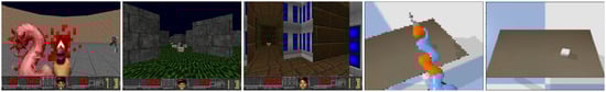
Figure 1.
States of the different environments used in this paper, from left to right: three ViZDoom environments (Defend the Center (DTC), Health Gathering Supreme (HGS), and My Way Home (MWH)) and two PyBullet environments (localization and reaching).
In these environments, the agent usually needs information about past observations to fully understand its state. This has been achieved by stacking frames or by adding Long Short-Term Memory (LSTM) layers [2]. However, stacking frames cannot capture dependencies that are too long, and adding recurrences complicates training and does not necessarily result in better performances in visual RL [3,4,5,6,7]. Nonetheless, LSTM can still be essential when its input is shaped to give tasks-related information [8,9,10,11]. Furthermore, with raw images as inputs, the network must extract reward-related features and predict value functions, which causes interference difficulties when learned simultaneously with only RL loss.
State Representation Learning (SRL) methods learn features of the environment and use the extracted features to solve RL tasks [12]. It has the advantage of speeding up the RL training due to lower dimension inputs and allowing a free molding of retrieved features as desired. Nevertheless, using SRL for image representation applied to RL necessitates training many networks with numerous losses, and prior environmental knowledge is frequently needed to improve the utility of the extracted features. In fact, using CNN to extract features from images, without prior knowledge, does not guarantee the extraction of reward-related characteristics, which can be disastrous for training an agent.
In this paper, we introduce the VRBFN, a light network composed of a generic untrained visual extractor and a Multi-Layer Perceptron (MLP), as an alternative to SRL approaches that learn feature extraction to address visual RL problems. Our visual extractor gave local and sparse features using Radial Basis Functions (RBFs). This extraction is then fed to an MLP trained with Proximal Policy Optimization (PPO) [13], an on-policy algorithm, to learn values of interest. This work extends our previous results [14] on more challenging partially observable environments and provides an extensive comparison with backbone methods of this field. The tasks addressed here come from ViZDoom [15], which offers a fast framework to train agents in challenging 3-D first-person environments to solve different types of tasks like mazes, shooting, and gathering objects. Moreover, to expand the diversity of tasks and situations, we developed two first-person challenges in PyBullet, which is a Python module for physics simulation for robotics, games, visual effects, and machine learning (more details can be found in [16]). Two tasks have been explored: one is a localization task with a camera, and the other is a reaching task with a Kuka arm.
The paper is organized as follows: after introducing the key concepts and related works, we describe the visual radial basis function Network design. Then, we present the different learned tasks, followed by a brief overview of the classical approaches we have used to challenge the VRBFN. Afterward, we discuss these comparison results and show the supremacy of the VRBFN in terms of performances and agent behavior in the different proposed environments. We also highlight the sparsity of our extraction and the robustness of the VRBFN to image scale and noise. We conclude with a discussion of the possible applications and perspectives of this method.
2. Related Work on Visual Reinforcement Learning
In RL, an agent in a state takes action according to its policy . Once the action is performed in the environment, the agent receives a new state with an associated reward . In the case of episodic RL, a Boolean variable D, which indicates whether the episode is finished or not, is given to the agent. The goal of the agent is to find a policy that maximizes the discounted cumulative long-term reward , where is the discounted rate determining the actual value of the future reward. In this paper, as we did not focus on the RL algorithms, we choose to learn RL tasks with proximal policy optimization (more details on this algorithm can be found in [13]). The latter has shown better performance than DQN [1] and A2C, the non-parallelized A3C [17]. A2C and A3C stand for Advantage Actor–Critic and Asynchronous Advantage Actor–Critic, respectively. They are famous algorithms in the RL technique consisting of two elements: the actor, which selects actions, and the critic, which evaluates them by calculating the value function. The actor improves by choosing actions that yield higher rewards, while the critic assesses how the good action is relative to the average, using the value function to guide the actor towards better decisions [1,17]. These two algorithms are typically used in ViZDoom scenarios [18].
The introduction of the ViZDoom framework and the promising results of RL with vanilla DQN [15] have been followed by multiple competitions on a deathmatch scenario [19]. The complexity of the scenario has pushed participants to combine different networks and training rules such as human imitation, curriculum learning, goals, or hierarchical learning to win the proposed task. Indeed, ViZDoom proposes a challenging environment that vanilla algorithms can hardly solve [3,18,20,21]. However, such additional methods need more precise engineering and often use multiple networks, requiring massive computer power to be trained on raw image data. To reduce the cost of RL on visual data, SRL was introduced, and since then, several methods and algorithms have been developed. It is commonly known that an auto-encoder and deviated networks (VAE, β-VAE) are by far the most used networks to extract visual representations to solve RL [22,23,24,25]. Other competing methods exist in the literature, as presented in the overview paper [12]. However, when using an auto-encoder to extract features, we cannot guarantee the usefulness of the extraction to solve the task, hence adding prior knowledge such as hidden variables of the state (ammo, life, position, etc.) is essential [26,27,28]. This is also one of the key points in [9], which was the winner of the last ViZDoom competition. Nonetheless, prior knowledge is not always accessible, and CNN is often used as the extractor, which implies additional learning time. An alternative solution is to use pre-trained networks, for example, RESNet, to preprocess the raw image before feeding an MLP [29,30,31,32]. Random CNN can also be used to extract features from visual inputs, and it has been successfully used to generate curiosity in reinforcement learning [33].
In non-visual RL, learning compact representation has been achieved with lighter methods like tile coding [34], Fourier features [35], or the radial basis function [35,36,37,38]. They have a sparse representation, which is an advantage in RL [39]. Deep RL (DRL) can also benefit from sparse representation by using dense to sparse or sparse training methods with CNN [40]. In contrast, we show that our technique, like the lighter methods mentioned above, has a sparse representation by conception and does not require any training as compared to methods that use CNN for images. In addition, no convolution is used, which reduces training time and optimization complexity.
3. Presentation of the Visual Radial Basis Function Network
The idea is to model the agent visual receptors as multiple neurons localized on the image with 2-D Gaussian functions. As illustrated in Figure 2, like CNN, the core component of the VRBFN consists of an image-to-vector extractor and a two-layer MLP for action mapping. The main difference from other networks in RL is the fact that it employs a single layer to detect specific features in localized areas of the image, focusing on local colors/features rather than the overall structure. This model leads to sparse activation depending on the difference between the pixel under the attention area and the intensity center of the neuron. Using the Gaussian function as an image receptive field has been successfully used to reconstruct cortical images [41,42]. In [43], the authors used those filters combined with a fully connected layer to classify images. The obtained results are promising and the method facilitates object localization and novelty or déjà-vu detection. This might be useful for reinforcement learning. In our work, we adopted a similar strategy to extract local areas from the image. Like human eye receptors that are stimulated in a certain range of wavelengths, we apply on that attention area three RBFs, one for each canal of the RGB images, which will respond to a certain intensity.
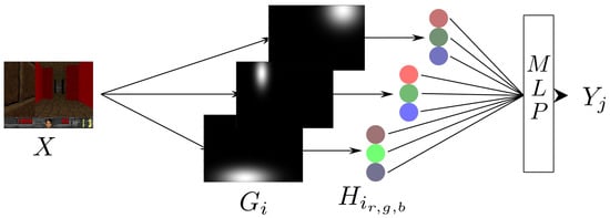
Figure 2.
Illustration of the visual radial basis function network for RGB input image X. For , in the example, is a receptive field, and are the activation functions for each color Gaussian unit. is the weight connecting the output to the activation .
The visual radial basis function network presented in Figure 2 is composed of two parts: an extractor that constructs local sparse stimulus H from the images and a Multilayer Perceptron (MLP) that learns a function from stimulus .
3.1. Visual Extraction into Sparse and Local Stimuli
The first part of the extraction used Image Receptive Field (IRF). This has been achieved by randomly generating 2D-Gaussian filters of amplitude one and multiplying them by the inputs. The random generation of the filters allows locality for each neuron. This issue can be enhanced by searching for the optimal generating distribution. This is beyond the scope of this paper. The receptive field of a neuron i for a pixel p in a state S (of shape ) with coordinates is defined as follows:
where define the center of the Gaussian function along a spatial dimension, and are the standard deviations. is the full matrix that defines the spatial attention area of a neuron. Given the attention area, the activation of the hidden neuron i is computed using a Gaussian RBF activation function weighted by :
where is the center, and the standard deviation of the RBF intensity Gaussian activation function. The symbol ⊙ is for the Hadamard product, i.e., the element-wise product. In that way, the closer a neuron’s center is to the intensity of the image under the attention area, the more its output will be close to one.
3.2. Learning Tasks with PPO from Stimuli
Proximal policy optimization is an actor–critic algorithm based on policy gradient methods. It has had considerable success, and a lot of enhancements have been proposed since its publication [13]. In this paper, we employed the original technique, but we concede that it can be improved when combined with the VRBFN, which is a processing module that can replace the convolutional part of the image-based network. Indeed, we used separate networks. On the one hand, the critic takes stimuli as inputs and outputs value functions indicating whether the state is acceptable or not in terms of the possible discounted future reward . On the other hand, the actor (policy) also takes stimuli as inputs but outputs continuous or discrete action.
- The continuous component: the mean of a Gaussian distribution from which the action is chosen with a standard deviation that is decreasing during the training, allowing more exploration at the beginning of the training.
- The discrete part: the softmax function, where the action is chosen depending on the max probability.
The goal of PPO is to maximize the policy improvement step in terms of success by keeping the updated policy close to the old one using a clipped objective function.
4. Experiments and Environmental Setup
Our VRBFN methods and other networks were developed using PyTorch on a Linux machine. The machine used for each training had a GPU Tesla V100 with 32 GB of memory, and we had access to four of them on the University Clermont Auvergne computing center Mesocenter. We did not parallelize the training processes. Each of them was performed on a single GPU. In the following, we describe the environmental setup and comparison methods.
4.1. ViZDoom Tasks
In our paper [14], basic and health gathering scenarios were solved with the VRBFN in a linear configuration without epsilon greedy and the target network. The promising results obtained motivated us to improve the scope of this method. We propose a study of its performances on more challenging, partially observable tasks with more comparison with baseline methods. We chose three ViZDoom tasks, and we designed two more realistic robotic tasks on the PyBullet simulator. All the ViZDoom and robotic tasks are learned with a discrete action space, including the empty action, and states; in addition, all experiments were in RGB with shape.
Defend the Center (DTC): The agent is in the middle of a circular room, and the goal is to shoot a maximum number of monsters. The latter spawn near the walls, far from the agent, and runs to kill the agent (see Figure 3). The action space is turn left, turn right, and shoot, and the agent is rewarded for killing a monster. The agent has 26 ammo, and the episode is finished when the agent dies. The challenges of this scenario depend on the enemies that can come from behind the agent and also on the limited number of ammunition. Moreover, monsters spawn far from the agent, as shown in Figure 3. To obtain the maximum reward, the agent should not miss a shot. He has to be precise or wait for the monsters to be close enough without dying. We give the agent a reward of for killing a monster and for dying. The maximum episode reward is 0.30 because the agent will always die due to the lack of ammo.
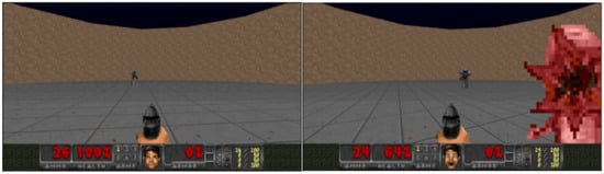
Figure 3.
Defend the center.
Health Gathering Supreme (HGS): The agent is in a labyrinth where the floor is hurting him, as illustrated in Figure 4. The goal is to survive by gathering health packs to recover life points. There is also a poison vial that makes him lose life points. The state space is {turn left, turn right, move forward}. The episode ends when the agent dies or when he reaches 2100 iterations. This scenario is complex because the health packs spawn randomly, so the agent can face empty areas. Moreover, the map is a maze, so the agent can be at dead ends.
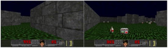
Figure 4.
Health gathering supreme.
In addition, the agent has to differentiate between poison vials and health packs to not lose life points and die fast. The agent has to survive, so each iteration is rewarded by , and his death is penalized by . As there is at maximum (=525 with ) iterations (see [15] for more details), the agent can reach a maximum episode reward of .
My Way Home (MWH): The agent spawns in one of the rooms of the labyrinth. Each room has different colors and textures, and the goal is to find the vest (see Figure 5). The episode ends when the agent reaches the vest or at most 2100 iterations. The action space is {turn left, turn right, move forward, move left, move right}. To solve this environment, the agent has to properly explore different rooms and learn the good path independently of the starting point. The agent receives a penalty of for each time step spent in the labyrinth and a reward of 1 for finding the vest.
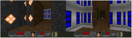
Figure 5.
My way home.
Moreover, we use the Done (D) flag only for death, so in health gathering supreme, if the agent reaches 525 steps without dying, the last steps will have . Similarly, on my way home, only when the agent finds the vest, anywhere else. Giving a penalty for dying by reaching the limit step can badly affect convergence in cases where there is no difference between a normal state and an end state, apart from the time step, which is not known by the agent.
4.2. Robotic Tasks
Two other common robotic tasks were tested: localizing and reaching an object. The environment and tasks were designed with the PyBullet simulator:
Localization: The goal is to move the camera to center around a white cube that has randomly appeared on a table. The cube is always present in the initial state of this environment, but the agent can progress to a state where it is no longer visible, as seen in the left state of Figure 6.
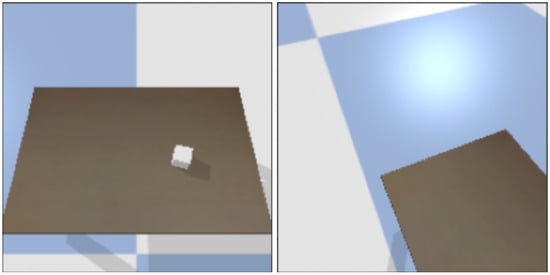
Figure 6.
Localization states.
The agent receives a reward of when it finds the cube and by otherwise. The agent controls the target of the camera by applying in the x- and/or y-dimensions on the table plan, resulting in a discrete space of 9 dimensions. The episode is reset after 100 iterations.
Reaching: The camera is locked on the cube, and the goal is to move a Kuka arm to reach the cube with the end effector. In this scenario (see Figure 7), the agent cannot see its arm at first, forcing it to perform a series of actions that will allow it to move its arm in front of the camera to gather useful visual information. In addition, the cube is randomly positioned on the table at the beginning of each episode. The agent receives a reward of 1 if it reaches the cube and otherwise. The agent can control the position of the 12 Kuka arm joints. For discrete space, we constrain the agent to move one joint by one with on position, resulting in 25 possible actions. The episode is reset after 200 iterations.
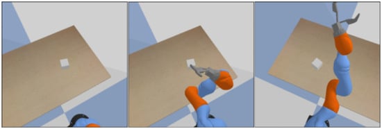
Figure 7.
Reaching states.
5. Methods for Comparison
Our VRBFN was tested on five scenarios to show its performance on diverse skills: exploring, gathering, precision, reaching, and localization. We compare our solution with five methods using the architectures presented in Figure 8.
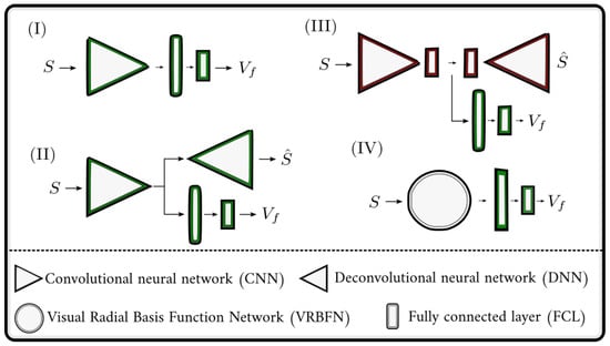
Figure 8.
Presentation of the four network architectures that are used in the experiments. Green represents networks trained during RL iteration, red pre-trained networks, and untrained networks without color. (I) is a CNN combined with two fully connected layers, (II) is the improvement of (I) when adding an auto-encoder, and (III) is a pre-trained auto-encoder that extracts features from inputs to feed an MLP for RL. The last network, (IV) is our VRBFN composed of the visual radial basis function extractor and an MLP of two fully connected layers.
We describe here the five methods that will be compared to the VRBFN. For each method, we specify the couple (number of trainable parameters, mean training time ):
- (I)
- Convolutional Neural Network (CNN): This is the baseline tool. We used a CNN followed by two fully connected layers to predict the value function . The networks count trainable parameters and the mean training time for one million iterations, on the defend the center (DTC) environment, for five seeds is = . (, ).
- (II)
- Convolutional Neural Network with Auto-encoder (CNNauto): Here, we add a reconstruction loss after the CNN bottleneck. The network will be trained to reconstruct the outputs and to predict . (, )
- (III)
- Autoencoder (Auto): Here, we pre-trained an auto-encoder, illustrated in red in Figure 8, to reconstruct the game inputs, and then we used the extracted features to predict . To train the auto-encoder, we gather 200k iterations from the game with random skip frames between 1 and 10, allowing more diversity in the dataset. We then train the auto-encoder for 100k steps (1 step corresponds to training on the 200k iterations data) with a batch size of 256 and a learning rate of . (, )
- (IV)
- Visual Radial Basis Function Network (VRBFN): For our method, we used the VRBFN to extract visual stimulus followed by two fully connected layers. (, )
- (V)
- Random CNN (CNNrdm): We used the same architecture as in (I) but all the weights of the convolutional layers are initialized with a normal distribution, , and never trained. (, )
- (VI)
- RESNet (RESNet): We used the pre-trained RESNet18 from PyTorch as the extractor. We remove the network’s last layer to get the features vector of 512 generated by trained convolutional layers. The network architecture looks like (IV) but with the RESNet18 in place of the VRBFN (, )
The CNN network used in Methods I, II, and V is composed of three convolutional layers of sizes with kernel size and strides . Linear rectified activations follow each layer, except for the output and the building of the latent vector in the auto-encoder. For the VRBFN in all experiments, we choose 1002 Gaussian neurons with and . In addition, we use distinct networks for the actor and the critic.
6. Results
All the curves in Figure 9 and Figure 10 are drawn with episodic rewards. This means that for one million steps, networks can achieve a different number of episodes depending on their behavior during training. In HGS, the longest curve is the worst because dying fast is penalized, like in DTC. In contrast, in all the other scenarios, long curves mean that the agent finishes more episodes and so solves the task more often. The drawn curves are an average over the five seeds with the mean in bold and the standard deviation in shadow. The training results are better for the VRBFN, ResNet, and CNNrdm methods, three methods that use pre-trained or untrained networks.
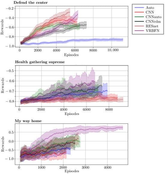
Figure 9.
Reward training curves for PPO methods in the three ViZDoom environments.
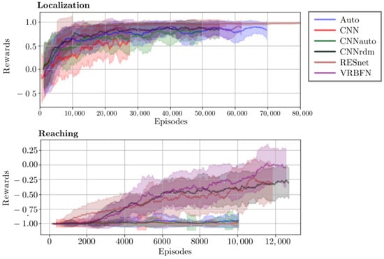
Figure 10.
Reward training curves for PPO methods in the two PyBullet handcrafted environments.
6.1. Vizdoom Tasks
For the three proposed ViZDoom environments, the testing results in Table 1 show that all the methods except the auto-encoder perform better or at least are equal to the CNN, with the best result for the VRBFN. Adding a reconstruction loss can help the CNN’s end-to-end training in scenarios that involve displacement and exploration. Moreover, it gives better results than the auto-encoder, where the extractor and policy are trained separately. Indeed, the features extracted by the auto-encoder cannot capture essential features such as the position of the monster or health pack far from the agent, which can be explained by the fact that the extractions are too general, as shown in Figure 11.

Table 1.
Rewards on 1000 episodes for ViZDoom tasks with PPO (image size: ) (mean ± std on 5 different initializations). The rewards reported here are those given by the original ViZDoom framework. In DFT, the agent receives +1 for killing a monster and −1 for dying. In HGS, the reward is the number of iterations reached by the agent before dying, and in MWH, the agent is penalized by −0.01 for each iteration and rewarded by +1 if it finds the vest.
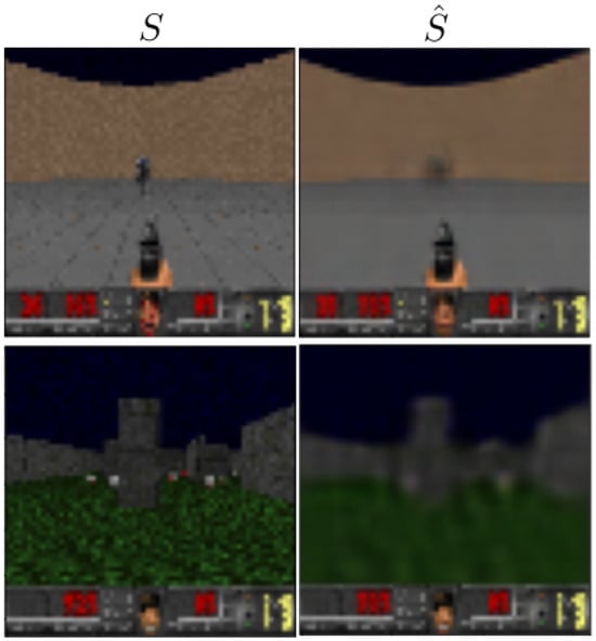
Figure 11.
Reconstruction of defend the center (up) and health gathering supreme (down) states from the auto-encoder.
The results of the CNNrdm are higher or similar to CNN and CNNauto, which show that the convolutional encoder used in CNN and Auto is unstable during the training and that guiding it to reconstruct the state is not enough to stabilize the extraction. From this observation, we can say that the CNN and CNNauto methods do not have enough time to learn good representation and state-action mapping in one million iterations. This is highlighted by the results of RESNet. It has been learned on general data for a long time, which allows the extraction to be more efficient and generic than the one obtained with CNN, CNNauto, and Auto. It should be noted that Gaussian distribution positioning is a key feature in the VRBFN’s performances, with varying results across different scenarios. For instance, the VRBFN excels in the ViZDoom scenario due to its ability to localize elements in images. It is effective at mid-range targeting but less so at long distances, unlike CNNs, which detect well from afar but lack precision. In health gathering, the VRBFN’s sparsity and locality characteristics help differentiate scenarios for better decision-making, outperforming CNNs for example. Furthermore, the VRBFN’s ability to recognize color patterns comes in handy in “My Way Home”. However, in the PyBullet scenario, the VRBFN’s strategy is less effective due to the cube’s movement. In addition, with the Kuka arm, the VRBFN’s strength lies in the ability to distinguish states, aiding in task execution.
Behavior in Vizdoom Environment
In defend the center, the CNN and CNNauto agents miss a lot of shots while trying to kill far monsters, but there are some seeds that favor the mid-/close-range shot that is easier to touch. In CNNrdm, the agents wait for the monster to come closer to shoot, which is supposed to be good behavior as ammunition is limited and missing a shot can dramatically decrease the episode reward. Nevertheless, the CNNrdm agent often dies with ammunition because too many monsters hurt it and the agent waits too long to shoot. For VRBFN and RESNet, the agents do not miss too many shots as they do not shoot far enemies but rather mid/close ones. The method using the pre-trained auto-encoder lacks success. It has some seeds that learn nothing and others that just shoot and turn, expecting a monster to be killed, and even just shoot without moving. For almost all the methods, except Auto, the agent always turns in the same direction, waiting for a monster to be in the shooting range.
In the health gathering supreme scenario, the reward is positive for each iteration. This kind of reward is harder to maximize with RL than the reward in the two other scenarios. In fact, even if the agent takes a poison vial or does nothing, it will be positively rewarded. The only negative reward comes when the agent dies. To fully complete the task, the agent has to deal with delayed rewards. Furthermore, because information about its life is difficult to obtain on the screen, the dying states will be almost identical to the rewarding states that appear during episodes. Nonetheless, methods like CNNrdm or the VRBFN achieve good scores compared to others; agents are able to run away from a dead end, turn when facing walls, and from time to time avoid isolated poison vials. In some seeds, VRBFN achieves the maximum reward in most of the episodes. The CNN and RESNet have the poorest results; the agents can collect health packs but always end up on the wall. CNNauto and Auto perform slightly better in some episodes by accumulating more health packs, but when the agent encounters several health packs or different corridors, the action decision is ambiguous, and the agent oscillates between multiple actions, causing him to lose time and die.
In my way home, CNN and Auto can hardly walk into the maze. Agents always get stuck in a room or on a wall, and few rewards can be gathered when the agent begins close to the vest. For CNNrdm, RESNet, and CNNauto, the agent gets less stuck but still can hardly find the vest when it appears far from it. The VRBFN method is the one performing the most on this task. The agent does not get stuck in the wall, can easily find the vest, and recovers from going in a bad direction.
6.2. Robotics Tasks
Both tasks have been designed to be partially observable, with sparse reward: positive if the agent succeeds, and negative anywhere else. In the localization task, we can observe in Figure 10 that only RESNet converges to one. Other methods struggle between 0.5 and 1. However, methods using extraction loss or untrained extractors show better learning performances than the CNN. Nonetheless, as those methods did not converge, the test results in Table 2 do not follow the training curves. Indeed, apart from RESNet and CNNrdm, which have representative results, the other methods have a huge standard deviation, which can be explained by the lack of convergence and can be corrected by adding some learning epochs. The second task, reachability, has been designed to be really complex and to expose the limitations of using only images as input.
Table 2.
Rewards on 1000 episodes for PyBullet tasks with PPO (image size: ) (mean ± std on 5 different initialization).
The reaching task can be seen as an extreme case of partial observability. In fact, in this scenario, the agent controls an arm through vision, and there are many observations where the Kuka arm is not present. As we can see in Figure 10, only the VRBFN, the RESNet, and the CNNrdm methods succeed in learning sub-optimal policy for some seeds, the CNNs are the worst method, closely followed by Auto and CNNauto, as shown in the test result in Table 2. CNN and CNNauto spend too much time trying to learn with images without the Kuka arm because it is hard to make it randomly move in front of the camera. Moreover, once it learns something about the initial state and succeeds in moving the arm in front of the camera, catastrophic forgetting occurs. On the contrary, the VRBFN and CNNrdm have a fixed extraction, which makes it easier for the agent to learn an action that will move the arm on the screen and then obtain a new activation pattern to learn new actions. Methods that use a pre-trained auto-encoder cannot yield good results. In fact, the pre-training is performed on random actions; thus, the network will not learn to correctly reproduce the arm because there will be fewer images with the arm than in the initial state. The RESNet extractor is able to give sufficient information to learn how to touch the cube in some episodes.
7. Properties and Characteristics of the Networks
The outcomes showcased in this paper highlight the network’s noteworthy benefits for practical uses. Using only two linear layers, the lightweight network effectively demonstrates rapid, accurate training at relatively low complexity. For the network to handle real-world applications, scalability and noise resilience are critical. Indeed, compared to simulations, real-world sensors can change over time and are more prone to noise. In these situations, a Convolutional Neural Network (CNN) would probably need to be retrained completely, whereas our network could simply need some minor fine-tuning if the output is still useful.
7.1. Robustness to Input Size
When working with images, it is interesting to test the agent’s adaptability to noise. We could add specific types of noise to the observations, such as Gaussian or salt-and-pepper noise, but these types of noise may be too specific. Instead, we chose to test the robustness of the agent against a commonly underestimated noise: the noise created when changing the size of images using the bilinear transformation. This type of noise frequently occurs when transferring learning to different sensors or simulators. For instance, in ViZDoom, visual observations can have different dimensions compared to other simulators.
In our study on ViZDoom, we initially chose the smallest observation size of 160 × 120, which we resized to 64 × 64 to accelerate learning. To assess robustness, we tested all methods on images that were twice as large, measuring 320 × 240, and subsequently scaled them down to 64 × 64. Under these conditions, when comparing the observations obtained during an episode of DTC, for example, we found a Mean Squared Error (MSE) of between the two types of images. We also examined the MSE between the feature extractions produced by each method. For the Auto method, the MSE was ; for RESNet, it was l for CNNrdm, it was ; and for VRBFN, it was . As highlighted in Table 3, these results indicate that VRBFN is the most robust to the noise caused by changes in image size, whereas representation learning methods are more affected by this type of noise. In order to quantify the influence of noise, we tested the methods on 100 episodes with noisy observations for each of the three scenarios. The VRBFN is much more noise-resistant than other methods. In MWH, for example, where there are not too many small details, the MSE of the images is around , and therefore, the results of the VRBFN are the same. However, for the other methods, even insignificant noise leads to a decrease in performances.
Table 3.
Rewards on ViZDoom scenario with image shape rescaled to .
Another test would involve assessing methods with larger images. However, this would pose a problem for agents with a CNN, as the size of the latent space would also increase, making it incompatible with the MLP. In the RESNet, a method is employed to address this issue by reducing the size of the latent space to a fixed dimension using pooling layers. To compare the RESNet, which utilizes this latent space reduction method, with our VRBFN, which is inherently adaptable to different image sizes without altering the meaning of its activations that we present in Table 4. It clearly demonstrates that the reduction method used in the RESNet for the latent space is not particularly effective, whereas our VRBFN network excels at adapting to different image sizes while maintaining the integrity of its activations.
Table 4.
Rewards on ViZDoom scenario with larger images for RESNet and VRBFN.
7.2. Sparsity
The VRBFN network exhibits sparse activation, where some neurons consistently have activations below a certain threshold, denoted as , for all states in a given scenario. Sparse activation resulting from neurons that are not in use has multiple advantages. First, lighter computations are made during training since inactive neurons do not contribute to forward or backward passes. Second, they may be removed after training in order to create a new, lighter network with fewer parameters without significantly sacrificing performance, which will result in quicker inference times. Lastly, during training, inactive neurons can renew, providing additional information and, as a result, increasing accuracy. The intricacy of the surroundings has a significant impact on the quantity of inactive neurons. For instance, more neurons are likely to activate in an environment with a greater variety of colors and textures. Table 5 presents the percentage of inactive neurons for different values of in each scenario. The data were obtained by randomly generating 1000 images (D) of the environment and examining the maximum activation (H) of each neuron based on the collected data. In DTC and HGS scenarios, the percentage of inactive neurons is similar, while in the MWH scenario, it differs. This discrepancy can be attributed to the diverse range of states in the MWH scenario, whereas the other scenarios feature a repeated design throughout the map. In the reaching environment, random actions result in unbalanced data, so we collected data using the best policy from the VRBFN to ensure an adequate number of images with the Kuka arm. To assess the usefulness of these Inactive Neurons (IN), we removed their connections and evaluated the lighter network’s performance in the scenario. The results shown in Table 5 indicate that testing without these IN neurons led to equal or better results except for localization, despite using fewer neurons. During training, these IN neurons would have near-zero connection weights, and gradient descent would not focus on them, potentially introducing noise to the output. However, it is important to note that should not exceed , as setting it too high would result in the loss of valuable information and degrade performances.
Table 5.
Percent of inactive neurons in the VRBFN and test without IN for each environment and for different activation thresholds . The results are mean and standard deviation over 5 different seeds.
8. Conclusions and Future Work
The presented results in the paper show that in general using untrained extractors has lots of benefits. It does not require state representational training, and it keeps stable extraction during the RL training in opposition to end-to-end training. Moreover, as the image is transformed to a smaller vector, the training time is reduced and only MLP are needed for RL training. Pre-trained extractors have the same advantages, but there are some conditions: the extractor has to be trained on generic data rather than on the scenario to obtain better genericity and performances, as shown by the result of Auto and RESNet methods. In contrast, using an end-to-end CNN is time-consuming as it will converge slowly, and solving partially observable visual tasks in end-to-end training does not seem to be accessible with vanilla algorithms. However, adding a reconstruction loss can help the CNN to converge in some cases, but the reconstruction loss is too general and not reward-related. An alternative would be, for instance, to use prior knowledge, like the health point or ammunition number in ViZDoom, as a target for the extraction.
Our proposition, the VRBFN, while having good performances on partially observable tasks, has advantageous capacities such as scalability or sparsity without any additional learning strategies or layers. These skills can be used for fine-tuning purposes, such as transferring knowledge on larger image input or by re-generating inactive neurons to obtain more information. There is still work to do on the distribution of the receptive field. Indeed, all our parameters are chosen randomly, which could be changed by an optimal distribution of the neuron’s attention areas. Future work should be conducted on the capacity to transfer knowledge learned in simulation to the real world by applying basic domain randomization. Our intuition for successful transfer learning resides in the robustness of our extraction to input variations. In addition, even when changing the image domains, the stimulus space stays unchanged. The perspectives of this work involve reducing the computational time required for the VRBFN model through parallel processing, especially for the reduction of the extraction time, which is the most critical factor in the training time of the VRBFN. This can be achieved by parallelizing the network, as each Gaussian operates independently of the others. In this case, the VRBFN stimuli can be calculated on different GPUs or CPUs. Additionally, currently, we use the entire image for the receptive field, but we can consider using localized patch receptive fields within the image. Significant effort and development are required before the models learned in simulations can be effectively transferred to real-world images. For instance, adapting the localization tasks to work with an actual camera necessitates further refinement.
Author Contributions
Conceptualization, C.T. and N.A.; Methodology, J.H., C.T. and N.A.; Software, J.H.; Investigation, J.H., C.T. and N.A.; Resources, C.T. and N.A.; Writing—original draft, J.H. and N.A.; Writing—review & editing, C.T. and N.A.; Supervision, C.T. and N.A.; Project administration, N.A.; Funding acquisition, C.T. and N.A. All authors have read and agreed to the published version of the manuscript.
Funding
This work has been supported by the AURA Region through the AUDACE2018 project of CPER 2015-2020. The authors are grateful to the Mésocentre Clermont Auvergne University for providing computing resources.
Data Availability Statement
Data is contained within the article.
Conflicts of Interest
The authors declare no conflict of interest.
References
- Mnih, V.; Kavukcuoglu, K.; Silver, D.; Rusu, A.A.; Veness, J.; Bellemare, M.G.; Graves, A.; Riedmiller, M.; Fidjeland, A.K.; Ostrovski, G.; et al. Human-level control through deep reinforcement learning. Nature 2015, 518, 529–533. [Google Scholar] [CrossRef] [PubMed]
- Hochreiter, S.; Schmidhuber, J. Long Short-Term Memory. Neural Comput. 1997, 9, 1735–1780. [Google Scholar] [CrossRef] [PubMed]
- Brejl, R.K.; Purwins, H.; Schoenau-Fog, H. Exploring Deep Recurrent Q-Learning for Navigation in a 3D Environment. Eai Endorsed Trans. Creat. Technol. 2018, 5, 153641. [Google Scholar] [CrossRef]
- Romac, C.; Béraud, V. Deep Recurrent Q-Learning vs Deep Q-Learning on a simple Partially Observable Markov Decision Process with Minecraft. arXiv 2019, arXiv:1903.04311. [Google Scholar]
- Moshayedi, A.J.; Roy, A.S.; Kolahdooz, A.; Shuxin, Y. Deep learning application pros and cons over algorithm deep learning application pros and cons over algorithm. EAI Endorsed Trans. AI Robot. 2022, 1, e7. [Google Scholar]
- Moshayedi, A.J.; Kolahdooz, A.; Liao, L. Unity in Embedded System Design and Robotics: A Step-by-Step Guide; CRC Press: Boca Raton, FL, USA, 2022. [Google Scholar]
- Durojaye, A.; Kolahdooz, A.; Nawaz, A.; Moshayedi, A.J. Immersive Horizons: Exploring the Transformative Power of Virtual Reality Across Economic Sectors. Eai Endorsed Trans. Robot. 2023, 2, e6. [Google Scholar] [CrossRef]
- OpenAI; Andrychowicz, M.; Baker, B.; Chociej, M.; Jozefowicz, R.; McGrew, B.; Pachocki, J.; Petron, A.; Plappert, M.; Powell, G.; et al. Learning Dexterous In-Hand Manipulation. arXiv 2018, arXiv:1808.00177. [Google Scholar]
- Lample, G.; Chaplot, D.S. Playing FPS games with deep reinforcement learning. In Proceedings of the 31st AAAI Conference on Artificial Intelligence, AAAI 2017, San Francisco, CA, USA, 4–9 February 2017; pp. 2140–2146. [Google Scholar] [CrossRef]
- Pathak, D.; Agrawal, P.; Efros, A.A.; Darrell, T. Curiosity-driven exploration by self-supervised prediction. In Proceedings of the 2017 IEEE Conference on Computer Vision and Pattern Recognition Workshops (CVPRW), Honolulu, HI, USA, 21–26 July 2017; Volume 6, pp. 4261–4270. [Google Scholar] [CrossRef]
- Moshayedi, A.J.; Uddin, N.M.I.; Khan, A.S.; Zhu, J.; Emadi Andani, M. Designing and Developing a Vision-Based System to Investigate the Emotional Effects of News on Short Sleep at Noon: An Experimental Case Study. Sensors 2023, 23, 8422. [Google Scholar] [CrossRef]
- Lesort, T.; Díaz-Rodríguez, N.; Goudou, J.F.; Filliat, D. State representation learning for control: An overview. Neural Netw. 2018, 108, 379–392. [Google Scholar] [CrossRef]
- Schulman, J.; Wolski, F.; Dhariwal, P.; Radford, A.; Klimov, O. Proximal Policy Optimization Algorithms. arXiv 2017, arXiv:1707.06347. [Google Scholar]
- Hautot, J.; Teuliere, C.; Azzaoui, N. Visual Radial Basis Q-Network. In Proceedings of the Third International Conference Pattern Recognition and Artificial Intelligence, ICPRAI 2022, Paris, France, 1–3 June 2022; Lecture Notes in Computer Science (Including Subseries Lecture Notes in Artificial Intelligence and Lecture Notes in Bioinformatics). Springer: Cham, Switzerland, 2022; Volume 13364, pp. 318–329. [Google Scholar] [CrossRef]
- Kempka, M.; Wydmuch, M.; Runc, G.; Toczek, J.; Jaskowski, W. ViZDoom: A Doom-based AI research platform for visual reinforcement learning. In Proceedings of the IEEE Conference on Computatonal Intelligence and Games, CIG, Santorini, Greece, 20–23 September 2016. [Google Scholar] [CrossRef]
- Coumans, E.; Bai, Y. Pybullet, a Python Module for Physics Simulation for Games, Robotics and Machine Learning, 2016–2021. Available online: http://pybullet.org (accessed on 4 October 2023).
- Mnih, V.; Badia, A.P.; Mirza, L.; Graves, A.; Harley, T.; Lillicrap, T.P.; Silver, D.; Kavukcuoglu, K. Asynchronous methods for deep reinforcement learning. In Proceedings of the 33rd International Conference on Machine Learning, ICML 2016, New York, NY, USA, 19–24 June 2016; Volume 48, pp. 1928–1937. [Google Scholar] [CrossRef]
- Olsson, M.; Malm, S.; Witt, K. Evaluating the Effects of Hyperparameter Optimization in VizDoom, Dissertation. Available online: https://www.diva-portal.org/smash/get/diva2:1679888/FULLTEXT01.pdf (accessed on 4 October 2023).
- Wydmuch, M.; Kempka, M.; Jaskowski, W. ViZDoom Competitions: Playing Doom From Pixels. IEEE Trans. Games 2018, 11, 248–259. [Google Scholar] [CrossRef]
- Akimov, D.; Makarov, I. Deep reinforcement learning with vizdoom first-person shooter? Ceur Workshop Proc. 2019, 2479, 3–17. [Google Scholar]
- Wu, M.; Ulrich, C.M.; Salameh, H. Training a Game AI with Machine Learning, Bachelor Project IT-University of Copenhagen. 2020. pp. 0–88. Dissertation. Available online: https://www.researchgate.net/publication/341655155_Training_a_Game_AI_with_Machine_Learning (accessed on 4 October 2023).
- Yarats, D.; Zhang, A.; Kostrikov, I.; Amos, B.; Pineau, J.; Fergus, R. Improving Sample Efficiency in Model-Free Reinforcement Learning from Images. In Proceedings of the 35th AAAI Conference on Artificial Intelligence, AAAI 2021, Virtually, 2–9 February 2021; Volume 35, pp. 10674–10681. [Google Scholar] [CrossRef]
- Li, Y.; Sycara, K.; Iyer, R. Object-sensitive Deep Reinforcement Learning. In Proceedings of the GCAI 2017. 3rd Global Conference on Artificial Intelligence, Miami, FL, USA, 18–22 October 2017; Benzmüller, C., Lisetti, C., Theobald, M., Eds.; EPiC Series in Computing. EasyChair: Manchester, GB, USA, 2017; Volume 50, pp. 20–35. [Google Scholar] [CrossRef]
- Lange, S.; Riedmiller, M.; Voigtländer, A. Autonomous reinforcement learning on raw visual input data in a real world application. In Proceedings of the International Joint Conference on Neural Networks, Brisbane, QLD, Australia, 10–15 June 2012. [Google Scholar] [CrossRef]
- Dittadi, A.; Träuble, F.; Wüthrich, M.; Widmaier, F.; Gehler, P.; Winther, O.; Locatello, F.; Bachem, O.; Schölkopf, B.; Bauer, S. Representation Learning for Out-of-Distribution Generalization in Reinforcement Learning. arXiv 2021, arXiv:2107.05686. [Google Scholar]
- Finn, C.; Tan, X.Y.; Duan, Y.; Darrell, T.; Levine, S.; Abbeel, P. Deep spatial autoencoders for visuomotor learning. In Proceedings of the 2016 IEEE International Conference on Robotics and Automation (ICRA), Stockholm, Sweden, 16–21 May 2016; pp. 512–519. [Google Scholar] [CrossRef]
- Leibfried, F.; Vrancx, P. Model-Based Regularization for Deep Reinforcement Learning with Transcoder Networks. arXiv 2018, arXiv:1809.01906. [Google Scholar]
- Zhong, Y.; Schwing, A.; Peng, J. Disentangling Controllable Object through Video Prediction Improves Visual Reinforcement Learning. arXiv 2020, arXiv:2002.09136. [Google Scholar]
- Parisi, S.; Rajeswaran, A.; Purushwalkam, S.; Gupta, A. The Unsurprising Effectiveness of Pre-Trained Vision Models for Control. arXiv 2022, arXiv:2203.03580. [Google Scholar]
- Xie, Z.; Lin, Z.; Li, J.; Li, S.; Ye, D. Pretraining in Deep Reinforcement Learning: A Survey. arXiv 2022, arXiv:2211.03959. [Google Scholar]
- Shah, R.; Kumar, V. RRL: Resnet as representation for Reinforcement Learning. arXiv 2021, arXiv:2107.03380. [Google Scholar]
- Elharrouss, O.; Akbari, Y.; Almaadeed, N.; Al-maadeed, S. Backbones-Review: Feature Extraction Networks for Deep Learning and Deep Reinforcement Learning Approaches. arXiv 2022, arXiv:2206.08016. [Google Scholar]
- Burda, Y.; Storkey, A.; Darrell, T.; Efros, A.A. Large-scale study of curiosity-driven learning. In Proceedings of the 7th International Conference on Learning Representations, ICLR 2019, New Orleans, LA, USA, 6–9 May 2019. [Google Scholar]
- Ghiassian, S.; Rafiee, B.; Lo, Y.L.; White, A. Improving performance in reinforcement learning by breaking generalization in neural networks. In Proceedings of the International Joint Conference on Autonomous Agents and Multiagent Systems, AAMAS, Auckland, New Zealand, 9–13 May 2020; pp. 438–446. [Google Scholar] [CrossRef]
- Li, Z. Fourier Features in Reinforcement Learning with Neural Networks. arXiv 2021, arXiv:2109.10623. [Google Scholar]
- Asadi, K.; Parr, R.E.; Konidaris, G.D.; Littman, M.L. Deep RBF value functions for continuous control. arXiv 2020, arXiv:2002.01883. [Google Scholar]
- Capel, N.; Zhang, N. Extended Radial Basis Function Controller for Reinforcement Learning. arXiv 2020, arXiv:2009.05866. [Google Scholar]
- Cetina, V.U. Multilayer perceptrons with radial basis functions as value functions in reinforcement learning. In Proceedings of the ESANN 2008 Proceedings, 16th European Symposium on Artificial Neural Networks—Advances in Computational Intelligence and Learning, Bruges, Belgium, 23–25 April 2008; pp. 161–166. [Google Scholar]
- Liu, V.; Kumaraswamy, R.; Le, L.; White, M. The utility of sparse representations for control in reinforcement learning. In Proceedings of the 33rd AAAI Conference on Artificial Intelligence, AAAI 2019, 31st Innovative Applications of Artificial Intelligence Conference, IAAI 2019 and the 9th AAAI Symposium on Educational Advances in Artificial Intelligence, EAAI 2019, Honolulu, HI, USA, 27 January–1 February 2019; pp. 4384–4391. [Google Scholar] [CrossRef]
- Graesser, L.; Evci, U.; Elsen, E.; Castro, P.S. The state of sparse training in deep reinforcement learning. In Proceedings of the International Conference on Machine Learning, PMLR, Baltimore, MD, USA, 17–23 July 2022; pp. 7766–7792. [Google Scholar]
- Balasuriya, S. A Computational Model of Space-Variant Vision Based on a Self-Organised Artificial Retina Tessellation. Ph.D. Thesis, University of Glasgow, Glasgow, UK, 2006. [Google Scholar]
- Boyd, L.C.; Popovic, V.; Siebert, J.P. Deep Reinforcement Learning Control of Hand-Eye Coordination with a Software Retina. In Proceedings of the 2020 International Joint Conference on Neural Networks, Glasgow, UK, 19–24 July 2020. [Google Scholar] [CrossRef]
- Buessler, J.L.; Smagghe, P.; Urban, J.P. Image receptive fields for artificial neural networks. Neurocomputing 2014, 144, 258–270. [Google Scholar] [CrossRef]
Disclaimer/Publisher’s Note: The statements, opinions and data contained in all publications are solely those of the individual author(s) and contributor(s) and not of MDPI and/or the editor(s). MDPI and/or the editor(s) disclaim responsibility for any injury to people or property resulting from any ideas, methods, instructions or products referred to in the content. |
© 2023 by the authors. Licensee MDPI, Basel, Switzerland. This article is an open access article distributed under the terms and conditions of the Creative Commons Attribution (CC BY) license (https://creativecommons.org/licenses/by/4.0/).