Generalized Permutants and Graph GENEOs

Abstract

This paper is part of a line of research devoted to developing a compositional and geometric theory of Group Equivariant Non-Expansive Operators (GENEOs) for Geometric Deep Learning. It has two objectives. The first objective is to generalize the notions of permutants and permutant measures, originally defined for the identity of a single “perception pair”, to a map between two such pairs. The second and main objective is to extend the application domain of the whole theory, which arose in the set-theoretical and topological environments, to graphs. This is performed using classical methods of mathematical definitions and arguments. The theoretical outcome is that, both in the case of vertex-weighted and edge-weighted graphs, a coherent theory is developed. Several simple examples show what may be hoped from GENEOs and permutants in graph theory and how they can be built. Rather than being a competitor to other methods in Geometric Deep Learning, this theory is proposed as an approach that can be integrated with such methods.

1. Introduction

In recent years, the need for an extension of Deep Learning to non-Euclidean domains has led to the development of Geometric Deep Learning (Section 1.1). This line of research focuses on applying neural networks to manifolds and graphs, making available new geometric models for artificial intelligence. In doing this, Geometric Deep Learning uses techniques from differential geometry, combinatorics, and algebra. In particular, it largely uses the concepts of group action and the equivariant operator (Section 1.2), which allow for a strong reduction in the number of parameters involved in machine learning.

1.1. Geometric Deep Learning

The basic idea of Geometric Deep Learning (GDL) [1,2,3] is to take into account the “geometric” nature of data to better focus the learning process and for parameter reduction. In fact, data may occur as sampled manifolds or as graphs, and the inherent structure may be essential for knowledge extraction. Moreover, functions defined from data may reveal essential features; this is, for example, the case with weighted graphs, the main object of the present study.

GDL should help to overcome the “black box syndrome” of deep learning, going towards “explainable AI” [4]. On this line of thought, one study [5] suggested shifting the focus from rough data to operators on data because operators are seen as elementary components that could substitute neurons in a neural network. Above all, operators represent the protagonist of explainable AI: the observer.

A prominent geometric feature is a symmetry with respect to a group of transformations, and this makes equivariance a necessary requirement when dealing with such data. The relevance of equivariance in GDL has been stressed in two recent studies [6,7].

1.2. Equivariant Operators

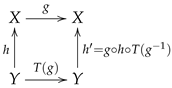
Consider an operator F on data $\Gamma$ (e.g., a convolution by a blurring kernel on an image) and a group G of transformations on $\Gamma$ (e.g., translations). Roughly said, F is equivariant with respect to G if F commutes with the transformations in G (in the example, first translating and then blurring gives the same result as first blurring and then translating).

The presence of symmetry with respect to a certain group of transformations is the most common reason for embedding equivariance in Deep Learning. For example, this is the case with the Euclidean, Lorenz, and Poincaré groups in the physical environments considered in [8]. Equivariance with respect to translations, rotations, and scaling is incorporated in deep learning for image processing and computational imaging in [9]. An SE(3)-equivariant deep learning model is introduced in [10] for protein binding prediction.

Group Equivariant Non-Expansive Operators (GENEOs, Definition 2) were introduced for building smart averages in the presence of such symmetries [5]; non-expansivity was required to express the information reduction and to grant convenient topological conditions. A way of producing GENEOs (preceding permutants) was first introduced in [11]. Permutants (Definition 3) and permutant measures (Definition 6) are general and flexible tools for building families of GENEOs. Bongard problems (typical intelligence tests) are faced through GENEOs in [12]. An application of GENEOs to protein pocket detection is mentioned in [13].

GENEOs inspired the introduction of Set Equivariant Operators (SEOs) for comparing structures within the framework of Persistent Homology in [14] and were a first step towards the comprehensive, formal description of artificial neural networks and their architectures [15,16].

1.3. Objectives

The present research had two objectives: giving a wider definition of permutant and extending the applicability of the whole theory to the domain of graphs.

The original definition of permutant concerned a single “perception pair” (Definition 1); here, it is defined for two perception pairs (Definition 4) and provides a construction method for GENEOs in this wider context (Theorem 1).

Since the beginning of GDL [1], the application of deep learning to data in the form of graphs appeared as a very interesting and promising development, both from theoretical and applied viewpoints. Much research is being done in this direction [17,18,19]. The main objective of the present paper is then to extend the application domain of the whole theory of GENEOs (generalized permutants included) to weighted graphs, where the weight function can be on vertices (Section 4.1) or edges (Section 4.2).

1.4. Outline

The rest of the paper is structured as follows. Section 2 recalls the mathematical setting, based on the concepts of perception pairs, GENEOs, and permutants. Section 3 introduces and describes the new concepts of generalized permutants and generalized permutant measures, proving that each of these can be used to build a GENEO (Theorems 1 and 3). In Section 4, the concepts of vertex-weighted-/edge-weighted-graph GENEOs are introduced, and the new mathematical model is illustrated with several examples. A section devoted to experiments (Section 5) shows how graph GENEOs may extract useful information from graphs, and how permutants can be built. Section 6 presents the final discussion.

2. The Set-Theoretical Setting

This section recalls the notions of perception pairs, GENEOs, and permutants as they were initially defined in the set-theoretical and topological environments [5,20], so that the generalizations defined in the following sections do not require consulting the references.

Let X be a non-empty set, $\Phi$ be a subspace of

$${\mathbb{R}}_b^X:=\{\phi :X\to \mathbb{R}\mid \phi \mathrm{is}\mathrm{bounded}\}$$

(1)

endowed with the topology induced by the $L^{\infty }$ distance

$$D_{\Phi }({\phi }_1,{\phi }_2):={\parallel {\phi }_1-{\phi }_2\parallel }_{\infty }=\underset{x\in X}{sup}|{\phi }_1\left(x\right)-{\phi }_2\left(x\right)|,{\phi }_1,{\phi }_2\in \Phi ,$$

(2)

and G be a subgroup of

$${\mathrm{Aut}}_{\Phi }\left(X\right):=\{g:X\to X\mid \mathrm{g}\mathrm{is}\mathrm{bijective}\mathrm{and}\phi \circ g,\phi \circ g^{-1}\in \Phi ,\forall \phi \in \Phi \}$$

(3)

with respect to the composition of functions.

Definition 1. 

We say that $(\Phi ,G)$ is a perception pair.

The elements $\phi$ of $\Phi$ are often called measurements. The fact that X is the common domain of all maps in $\Phi$ will be expressed as dom$(\Phi )=X$. The space $\Phi$ of measurements endows X and ${\mathrm{Aut}}_{\Phi }\left(X\right)$ (and, therefore, every subgroup G of ${\mathrm{Aut}}_{\Phi }\left(X\right)$) with topologies induced, respectively, by the extended pseudometrics

$$D_X(x_1,x_2):=\underset{\phi \in \Phi }{sup}|\phi \left(x_1\right)-\phi \left(x_2\right)|,x_1,x_2\in X$$

(4)

and

$$D_{\mathrm{Aut}}(f,g):=\underset{\phi \in \Phi }{sup}{D}_{\Phi }(\phi \circ f,\phi \circ g),f,g\in {\mathrm{Aut}}_{\Phi }\left(X\right).$$

(5)

It is known that each $g\in {\mathrm{Aut}}_{\Phi }\left(X\right)$ is an isometry of X [5].

Definition 2. 

Let $(\Phi ,G)$ and $(\Psi ,K)$ be perception pairs with $\text{dom}(\Phi )=X$ and $\text{dom}(\Psi )=Y$, and $T:G\to K$ be a group homomorphism. An operator $F:\Phi \to \Psi$ is said to be a group equivariant non-expansive operator (GENEO, for short) from $(\Phi ,G)$ to $(\Psi ,K)$ with respect to T if

$$F(\phi \circ g)=F\left(\phi \right)\circ T\left(g\right),\phi \in \Phi ,g\in G$$

(6)

and

$$\parallel F\left({\phi }_1\right)-F\left({\phi }_2\right){\parallel }_{\infty }\le {\parallel {\phi }_1-{\phi }_2\parallel }_{\infty },{\phi }_1,{\phi }_2\in \Phi .$$

(7)

For the sake of conciseness, we often write a GENEO as $(F,T):(\Phi ,G)\to (\Psi ,K)$. An operator that satisfies the first condition in this definition is called a group equivariant operator (GEO, for short), while one satisfying the second condition is said to be non-expansive.

The set ${\mathcal{F}}_T^{\mathrm{all}}$ of all GENEOs $(F,T):(\Phi ,G)\to (\Psi ,K)$, with respect to a fixed homomorphism T, is a metric space with the distance function given by

$$D_{\mathrm{GENEO}}(F_1,F_2):=\underset{\phi \in \Phi }{sup}{D}_{\Psi }(F_1\left(\phi \right),F_2\left(\phi \right)),F_1,F_2\in {\mathcal{F}}_T^{\mathrm{all}}.$$

(8)

A method to build GENEOs employing the concept of a permutant is illustrated in [20]. If G is a subgroup of ${\mathrm{Aut}}_{\Phi }\left(X\right)$, then the conjugation map ${\alpha }_g:{\mathrm{Aut}}_{\Phi }\left(X\right)\to {\mathrm{Aut}}_{\Phi }\left(X\right),$ given by $f\mapsto g\circ f\circ g^{-1}$, $g\in G$, plays a key role in this technique.

Definition 3. 

Let H be a finite subset of ${\mathrm{Aut}}_{\Phi }\left(X\right)$. We say that H is a permutant for G if $H=\varnothing$ or ${\alpha }_g\left(H\right)\subseteq H$ for every $g\in G$; i.e., ${\alpha }_g\left(f\right)=g\circ f\circ g^{-1}\in H$ for every $f\in H$ and $g\in G$.

Example 1. 

Let Φ be the set of all functions $\phi :X=S^1=\{(x,y)\in {\mathbb{R}}^2\mid x^2+y^2=1\}\to [0,1]$ that are non-expansive with respect to the Euclidean distances on $S^1$ and $[0,1]$. Let us consider the group G of all isometries of ${\mathbb{R}}^2$, restricted to $S^1$. If h is the clockwise rotation of ℓ radians for a fixed ℓ$\in \mathbb{R}$, then the set $H=\{h,h^{-1}\}$ is a permutant for G.

Other examples of permutants will be given in Example 10, Example 11, and Proposition 4.

We recall the following result. As usual, in the following, we will denote the set of all functions from the set A to the set B by the symbol $B^A$.

Proposition 1. 

Let $(\Phi ,G)$ be a perception pair with $\text{dom}(\Phi )=X$. If H is a non-empty permutant for $G\subseteq {\mathrm{Aut}}_{\Phi }\left(X\right)$, then the restriction to Φ of the operator $F:{\mathbb{R}}^X\to {\mathbb{R}}^X$ defined by

$$F\left(\phi \right):=\frac{1}{\left|H\right|}\sum _{h\in H}\phi \circ h$$

(9)

is a GENEO from $(\Phi ,G)$ to $(\Phi ,G)$ with respect to $T=i{d}_G$, provided that $F(\Phi )\subseteq \Phi$.

3. Generalized Permutants in the Set-Theoretical Setting

As revealed in Section 2, the notion of a permutant originally referred to a single perception pair. This section introduces a generalization of the concept of a permutant to the case of distinct perception pairs $(\Phi ,G)$ and $(\Psi ,K)$, and shows how it can be used to populate the space of GENEOs. In particular, Section 3.1 defines an equivalence relation among maps and recognizes a generalized permutant as a union of equivalence classes; Section 3.2 connects this notion with the action of the group G; and Section 3.3 recalls (Definition 6) and generalizes (Definition 7) the notion of a permutant measure to this new context.

Definition 4. 

Let $(\Phi ,G)$, $\mathrm{dom}(\Phi )=X$ and $(\Psi ,K)$, $\mathrm{dom}(\Psi )=Y$ be perception pairs and $T:G\to K$ be a group homomorphism. A finite set $H\subseteq X^Y$ of functions $h:Y\to X$ is called a generalized permutant for T if $H=\varnothing$ or $g\circ h\circ T\left(g^{-1}\right)\in H$ for every $h\in H$, and every $g\in G$.

In this case, we have the following commutative diagram:

(10)

We observe that the map $h\mapsto g\circ h\circ T\left(g^{-1}\right)$ is a bijection from H to H for any $g\in G$.

Definition 4 extends Definition 3 in two different directions. First, it does not require that the origin perception pair $(\Phi ,G)$ and the target perception pair $(\Psi ,K)$ coincide. Second, it does not require that the elements of the set H are bijections. In Section 5.2, we will see how the concept of generalized permutant can be applied.

Example 2. 

Let $X,Y$ be two non-empty finite sets, with $Y\subseteq X$. Let G be the group of all permutations of X that preserve Y, and K be the group of all permutations of Y. Set $\Phi ={\mathbb{R}}^X$ and $\Psi ={\mathbb{R}}^Y$. Assume that $T:G\to K$ takes each permutation of X to its restriction to Y. Define H as the set of all functions $h:Y\to X$ such that the cardinality of $\mathrm{Im}h$ is smaller than a fixed integer m. Then H is a generalized permutant for T.

In the following two subsections, we will express two other ways to look at generalized permutants, beyond their definition. To this end, we will assume that two perception pairs $(\Phi ,G)$, $(\Psi ,K)$ and a group homomorphism $T:G\to K$ are given, with $\mathrm{dom}(\Phi )=X$ and $\mathrm{dom}(\Psi )=Y$.

3.1. Generalized Permutants as Unions of Equivalence Classes

In view of Definition 4, we can define an equivalence relation ∼ on $X^Y$:

Definition 5. 

Let $h,h^{\prime }\in X^Y$. We say that h is equivalent to $h^{\prime }$, and write $h\sim h^{\prime }$, if there is a $g\in G$ such that $h^{\prime }=g\circ h\circ T\left(g^{-1}\right)$.

It is easy to see that ∼ is indeed an equivalence relation on $X^Y$.

Proposition 2. 

A subset H of $X^Y$ is a generalized permutant for T if and only if H is a (possibly empty) union of equivalence classes for ∼.

Proof. 

Assume that H is a generalized permutant for T. If $h\in H$ and $h\sim h^{\prime }\in X^Y$, then the definition of the relation ∼ and the definition of generalized permutant imply that $h^{\prime }\in H$ as well, and, therefore, H is a union of equivalence classes for ∼. Conversely, if H is a union of equivalence classes for the relation ∼, $h\in H$, and $g\in G$, then $g\circ h\circ T\left(g^{-1}\right)\in H$, since $g\circ h\circ T\left(g^{-1}\right)\sim h$. As a consequence, H is a generalized permutant for T. □

3.2. Generalized Permutants as Unions of Orbits

The map $\alpha :G\times X^Y\to X^Y$ taking $(g,f)$ to $g\circ f\circ T\left(g^{-1}\right)$ is a left group action, since $\alpha ({\mathrm{id}}_X,f)={\mathrm{id}}_X\circ f\circ T\left({\mathrm{id}}_X^{-1}\right)=f$ and $\alpha (g_2,\alpha (g_1,f))=\alpha (g_2,g_1\circ f\circ T\left(g_1^{-1}\right))=g_2\circ (g_1\circ f\circ T\left(g_1^{-1}\right))\circ T\left(g_2^{-1}\right)=(g_2\circ g_1)\circ f\circ T\left({(g_2\circ g_1)}^{-1}\right)=\alpha (g_2\circ g_1,f)$. For every $f\in X^Y$, the set $O\left(f\right):=\left\{\alpha \right(g,f):g\in G\}$ is called the orbit of f. By observing that $O\left(f\right)$ is the equivalence class of f in $X^Y$ for ∼, from Proposition 2 the following result immediately follows.

Proposition 3. 

A subset H of $X^Y$ is a generalized permutant for T if and only if H is a (possibly empty) union of orbits for the group action α.

The main use of the concept of generalized permutants is expressed by the following theorem, extending Proposition 1.

Theorem 1. 

Let $(\Phi ,G)$, $\mathrm{dom}(\Phi )=X$ and $(\Psi ,K)$, $\mathrm{dom}(\Psi )=Y$ be perception pairs, $T:G\to K$ a group homomorphism, and H be a generalized permutant for T. Then the restriction to Φ of the operator $F:{\mathbb{R}}^X\to {\mathbb{R}}^Y$ defined by

$$F\left(\phi \right):=\frac{1}{\left|H\right|}\sum _{h\in H}\phi \circ h$$

(11)

is a GENEO from $(\Phi ,G)$ to $(\Psi ,K)$ with respect to T provided $F(\Phi )\subseteq \Psi$.

Proof. 

Let $\phi \in \Phi$ and $g\in G$. Then, by the definition of a generalized permutant and the change of variable $h^{\prime }=g\circ h\circ T\left(g^{-1}\right)$, we have

$$\begin{array}{cc}\hfill F(\phi \circ g)& :=\frac{1}{\left|H\right|}\sum _{h\in H}(\phi \circ g)\circ h\hfill \\ \hfill & =\frac{1}{\left|H\right|}\sum _{h\in H}\phi \circ g\circ h\circ T\left(g^{-1}\right)\circ T\left(g\right)\hfill \\ \hfill & =\frac{1}{\left|H\right|}\sum _{h^{\prime }\in H}\phi \circ h^{\prime }\circ T\left(g\right)\hfill \\ \hfill & =F\left(\phi \right)\circ T\left(g\right)\hfill \end{array}$$

(12)

whence F is equivariant.

If ${\phi }_1,{\phi }_2\in \Phi$, then

$$\begin{array}{cc}\hfill {∥F\left({\phi }_1\right)-F\left({\phi }_2\right)∥}_{\infty }& ={∥\frac{1}{\left|H\right|}\sum _{h\in H}{\phi }_1\circ h-\frac{1}{\left|H\right|}\sum _{h\in H}{\phi }_2\circ h∥}_{\infty }\hfill \\ \hfill & =\frac{1}{\left|H\right|}{\parallel \sum _{h\in H}({\phi }_1\circ h-{\phi }_2\circ h)\parallel }_{\infty }\hfill \\ \hfill & \le \frac{1}{\left|H\right|}\sum _{h\in H}{\parallel {\phi }_1\circ h-{\phi }_2\circ h\parallel }_{\infty }\hfill \\ \hfill & \le \frac{1}{\left|H\right|}\sum _{h\in H}{\parallel {\phi }_1-{\phi }_2\parallel }_{\infty }\hfill \\ \hfill & =\frac{1}{\left|H\right|}\left|H\right|{\parallel {\phi }_1-{\phi }_2\parallel }_{\infty }\hfill \\ \hfill & =\parallel {\phi }_1-{\phi }_2{\parallel }_{\infty }\hfill \end{array}$$

(13)

whence F is non-expansive. Relations (12) and (13) prove that F is indeed a GENEO. □

3.3. Generalized Permutant Measures

As shown in [21], the concept of permutants can be extended to the that of permutant measures, provided that the set X is finite. This is done by the following definition, referring to a subgroup G of the group $\mathrm{Aut}\left(X\right)$ of all permutations of the set X, and to the perception pair $({\mathbb{R}}^X,G)$.

Definition 6 

([21]). A finite signed measure μ on $\mathrm{Aut}\left(X\right)$ is called a permutant measure with respect to G if each subset H of $\mathrm{Aut}\left(X\right)$ is measurable and μ is invariant under the conjugation action of G (i.e., $\mu \left(H\right)=\mu \left(gH{g}^{-1}\right)$ for every $g\in G$).

With a slight abuse of notation, we will denote by $\mu \left(h\right)$ the signed measure of the singleton $\left\{h\right\}$ for each $h\in \mathrm{Aut}\left(X\right)$. The next example shows how we can apply Definition 6.

Example 3. 

Let us consider the set X of the vertices of a cube in ${\mathbb{R}}^3$, and the group G of the orientation-preserving isometries of ${\mathbb{R}}^3$ that take X to X. Set $T={\mathrm{id}}_G$. Let ${\pi }_1,{\pi }_2,{\pi }_3$ be the three planes that contain the center of mass of X and are parallel to a face of the cube. Let $h_i:X\to X$ be the orthogonal symmetry with respect to ${\pi }_i$, for $i\in \{1,2,3\}$. We have that the set $\{h_1,h_2,h_3\}$ is an orbit under the action expressed by the map α defined in Section 3.2. We can now define a permutant measure μ on $\mathrm{Aut}\left(X\right)$ by setting $\mu \left(h_1\right)=\mu \left(h_2\right)=\mu \left(h_3\right)=c$, where c is a positive real number, and $\mu \left(h\right)=0$ for any $h\in \mathrm{Aut}\left(X\right)$ with $h\notin \{h_1,h_2,h_3\}$. We also observe that while the cardinality of G is 24, the cardinality of the support $\mathrm{supp}\left(\mu \right):=\{h\in \mathrm{Aut}(X):\mu (h)\ne 0\}$ of the signed measure μ is 3.

The concept of permutant measures is important because it makes available the following representation result.

Theorem 2. 

Assume that $G\subseteq \mathrm{Aut}\left(X\right)$ transitively acts on the finite set X and F is a map from ${\mathbb{R}}^X$ to ${\mathbb{R}}^X$. The map F is a linear, group equivariant, non-expansive operator from $({\mathbb{R}}^X,G)$ to $({\mathbb{R}}^X,G)$ with respect to the homomorphism ${\mathrm{id}}_G:G\to G$ if and only if a permutant measure μ exists such that $F\left(\phi \right)={\sum }_{h\in \mathrm{Aut}\left(X\right)}\phi \circ h^{-1}\mu \left(h\right)$ for every $\phi \in {\mathbb{R}}^X$, and ${\sum }_{h\in \mathrm{Aut}\left(X\right)}\left|\mu \left(h\right)\right|\le 1$.

We now state a definition that extends the concept of permutant measures.

Definition 7. 

Let X, Y be two finite non-empty sets. Let us choose a subgroup G of $\mathrm{Aut}\left(X\right)$, a subgroup K of $\mathrm{Aut}\left(Y\right)$, and a homomorphism $T:G\to K$. A finite signed measure μ on $X^Y$ is called a generalized permutant measure with respect to T if each subset H of $X^Y$ is measurable and $\mu \left(g\circ H\circ T\left(g^{-1}\right)\right)=\mu \left(H\right)$ for every $g\in G$.

Definition 7 extends Definition 6 in two different directions. First, it does not require that the origin perception pair $({\mathbb{R}}^X,G)$ and the target perception pair $({\mathbb{R}}^Y,K)$ coincide. Second, the measure $\mu$ is not defined on $\mathrm{Aut}\left(X\right)$ but on the set $X^Y$.

Example 4. 

Let $X,Y$ be two non-empty finite sets, with $Y\subseteq X$. Let G be the group of all permutations of X that preserve Y, and K be the group of all permutations of Y. Set $\Phi ={\mathbb{R}}^X$ and $\Psi ={\mathbb{R}}^Y$. Assume that $T:G\to K$ takes each permutation of X to its restriction to Y. For any positive integer m, define $H_m$ as the set of all functions $h:Y\to X$ such that the cardinality of $\mathrm{Im}h$ is equal to m. For each $h\in H_m$, let us set $\mu \left(h\right):=\frac{1}{m\left|H_m\right|}$. Then μ is a generalized permutant measure with respect to T.

We can prove the following result, showing that every generalized permutant measure allows us to build a GENEO between perception pairs.

Theorem 3. 

Let X, Y be two finite non-empty sets. Let us choose a subgroup G of $\mathrm{Aut}\left(X\right)$, a subgroup K of $\mathrm{Aut}\left(Y\right)$, and a homomorphism $T:G\to K$. If μ is a generalized permutant measure with respect to T, then the map $F_{\mu }:{\mathbb{R}}^X\to {\mathbb{R}}^Y$ defined by setting $F_{\mu }\left(\phi \right):={\sum }_{f\in X^Y}\phi \circ f\mu \left(f\right)$ is a linear GEO from $(\Phi ,G)$ to $(\Psi ,K)$ with respect to T. If ${\sum }_{f\in X^Y}\left|\mu \left(f\right)\right|\le 1$, then F is a GENEO.

Proof. 

It is immediate to check that $F_{\mu }$ is linear. Moreover, by applying the change of variable $\widehat{f}=g\circ f\circ T\left(g^{-1}\right)$ and the equality $\mu \left(g\circ f\circ T\left(g^{-1}\right)\right)=\mu \left(f\right)$, for every $\phi \in {\mathbb{R}}^X$ and every $g\in G$ we get

$$\begin{array}{cc}\hfill F_{\mu }(\phi \circ g)& =\sum _{f\in X^Y}\phi \circ g\circ f\mu \left(f\right)\hfill \\ \hfill & =\sum _{f\in X^Y}\phi \circ g\circ f\circ T\left(g^{-1}\right)\circ T\left(g\right)\mu (g\circ f\circ T\left(g^{-1}\right))\hfill \\ \hfill & =\sum _{\widehat{f}\in X^Y}\phi \circ \widehat{f}\circ T\left(g\right)\mu \left(\widehat{f}\right)\hfill \\ \hfill & =F_{\mu }\left(\phi \right)\circ T\left(g\right)\hfill \end{array}$$

(14)

since the map $f\mapsto g\circ f\circ T\left(g^{-1}\right)$ is a bijection from $X^Y$ to $X^Y$. This proves that $F_{\mu }$ is equivariant.

If ${\sum }_{f\in X^Y}\left|\mu \left(f\right)\right|\le 1$,

$$\begin{array}{cc}\hfill \parallel F_{\mu }{\left(\phi \right)\parallel }_{\infty }& ={∥\sum _{f\in X^Y}\phi \circ f\mu \left(f\right)∥}_{\infty }\hfill \\ \hfill & \le \sum _{f\in X^Y}{∥\phi \circ f∥}_{\infty }\left|\mu \left(f\right)\right|\hfill \\ \hfill & \le \sum _{f\in X^Y}{∥\phi ∥}_{\infty }\left|\mu \left(f\right)\right|\hfill \\ \hfill & ={\parallel \phi \parallel }_{\infty }\sum _{f\in X^Y}\left|\mu \left(f\right)\right|\hfill \\ \hfill & \le {\parallel \phi \parallel }_{\infty }.\hfill \end{array}$$

(15)

This implies that the linear map $F_{\mu }$ is non-expansive. Relations (14) and (15) prove that F is a GENEO, concluding the proof. □

The condition $\left|\mathrm{supp}\right(\mu \left)\right|\ll \left|G\right|$ is not rare in applications (cf., e.g., Example 3) and is the main reason to build GEOs utilizing (generalized) permutant measures, instead of using the representation of GEOs as G-convolutions and integrating on possibly large groups.

In the following, the aforementioned concepts will be applied to graphs. For the sake of simplicity, we will drop the word “generalized” and use the expression “graph permutant”.

4. GENEOs on Graphs

The definitions of perception pairs (Definition 1), (generalized) permutants (Definition 3, Definition 4), and GENEOs (Definition 2) can be easily applied in a graph-theoretic setting. In most applications where data occur as graphs, these are endowed with a real function (“weight”) defined either on vertices or on edges. Section 4.1 develops a model for graphs with weights assigned to their vertices ($\mathrm{vw}$-graphs, for short), and Section 4.2 does the same for graphs with weights assigned to their edges ($\mathrm{ew}$-graphs, for short), often called “weighted graphs” in the literature. The vertex model has implications for the rapidly growing field of graph convolutional neural networks, while the edge model owes its significance to the widely recognized importance of weighted graphs. For either model, several simple examples are provided.

As a graph [22], we shall mean a triple $\Gamma =(V_{\Gamma },E_{\Gamma },{\psi }_{\Gamma })$, where ${\psi }_{\Gamma }$ assigns to each edge of $E_{\Gamma }$ the unordered pair of its end vertices in $V_{\Gamma }$. Since we only consider simple graphs (i.e., with no loops and no multiple edges) we write $e=\{A,B\}$ to mean ${\psi }_{\Gamma }\left(e\right)=\{A,B\}$. Let us recall that an automorphism g of $\Gamma$ is a pair $g=(g_V,g_E)$, where $g_V:V_{\Gamma }\to V_{\Gamma }$ and $g_E:E_{\Gamma }\to E_{\Gamma }$ are bijections respecting the incidence function ${\psi }_{\Gamma }$. The group $\mathrm{Aut}(\Gamma )$ of all automorphisms of $\Gamma$ induces two particular subgroups, here denoted as $\mathrm{Aut}\left(V_{\Gamma }\right)$ and $\mathrm{Aut}\left(E_{\Gamma }\right)$, of the groups of permutations of $V_{\Gamma }$ and of $E_{\Gamma }$. We represent permutations as cycle products.

For any $k\in \mathbb{N}$, put ${\mathbb{N}}_k:=\{1\le i\le k\mid i\in \mathbb{N}\}.$

Let a graph $\Gamma =(V_{\Gamma },E_{\Gamma },{\psi }_{\Gamma })$ with n vertices and m edges be given. By fixing an indexing of the vertices (resp. edges), we can identify $\mathrm{Aut}\left(V_{\Gamma }\right)$ (resp. $\mathrm{Aut}\left(E_{\Gamma }\right)$) with some subgroup of $S_n$ (resp. $S_m$), for the sake of simplicity. Analogously, a real function defined on $V_{\Gamma }$ (resp. $E_{\Gamma }$) will be represented as an n-tuple (resp. m-tuple) of real numbers. Regardless, we shall denote vertices (resp. edges) by consecutive capital (resp. lowercase) letters and not by numerical indexes.

In this section, a space ${\Phi }_{V_{\Gamma }}$ of real valued functions on $V_{\Gamma }$ will be considered as a subspace of ${\mathbb{R}}^n$ endowed with the sup-norm ${\parallel ·\parallel }_{\infty }$; i.e., the real valued functions $\phi \in {\Phi }_{V_{\Gamma }}$ on the vertex set $V_{\Gamma }$ are given by vectors $\phi =({\phi }^1,{\phi }^2,\cdots ,{\phi }^n)$ of length n. Analogously, the symbol ${\Phi }_{E_{\Gamma }}$ will refer to a subspace of ${\mathbb{R}}^m$ endowed with the sup-norm; i.e., the real valued functions $\phi \in {\Phi }_{E_{\Gamma }}$ on the edge set $E_{\Gamma }$ are given by vectors $\phi =({\phi }^1,{\phi }^2,\cdots ,{\phi }^m)$ of length m.

Let G be a subgroup of the group $\mathrm{Aut}\left(V_{\Gamma }\right)$ (resp. $\mathrm{Aut}\left(E_{\Gamma }\right)$) corresponding to the group of all graph automorphisms of $\Gamma$. By the previous convention, the elements of G can be considered to be permutations of the set ${\mathbb{N}}_n$ (resp. ${\mathbb{N}}_m$).

4.1. GENEOs on Graphs Weighted on Vertices

The concepts of perception pairs, GEOs/GENEOs, and generalized permutants are applied to $\mathrm{vw}$-graphs in Definitions 8, 9, and 10, respectively.

Definition 8. 

Let ${\Phi }_{V_{\Gamma }}$ be a set of functions from $V_{\Gamma }$ to $\mathbb{R}$ and G be a subgroup of $\mathrm{Aut}\left(V_{\Gamma }\right)$. If $({\Phi }_{V_{\Gamma }},G)$ is a perception pair, we will call it a $\mathrm{vw}$-graph perception pair for $\Gamma =(V_{\Gamma },E_{\Gamma },{\psi }_{\Gamma })$, and will write $\mathrm{dom}\left({\Phi }_{V_{\Gamma }}\right)=V_{\Gamma }$.

Definition 9. 

Let $({\Phi }_{V_{{\Gamma }_1}},G_1)$ and $({\Phi }_{V_{{\Gamma }_2}},G_2)$ be two $\mathrm{vw}$-graph perception pairs and $T:G_1\to G_2$ be a group homomorphism. If $F:{\Phi }_{V_{{\Gamma }_1}}\to {\Phi }_{V_{{\Gamma }_2}}$ is a GEO (resp. GENEO) from $({\Phi }_{V_{{\Gamma }_1}},G_1)$ to $({\Phi }_{V_{{\Gamma }_2}},G_2)$ with respect to T, we will say that F is a $\mathrm{vw}$-graph GEO (resp. $\mathrm{vw}$-graph GENEO).

Definition 10. 

Let $({\Phi }_{V_{{\Gamma }_1}},G_1)$ and $({\Phi }_{V_{{\Gamma }_2}},G_2)$ be two $\mathrm{vw}$-graph perception pairs and $T:G_1\to G_2$ be a group homomorphism. We say that $H\subseteq {V_{{\Gamma }_1}}^{V_{{\Gamma }_2}}$ is a $\mathrm{vw}$-graph permutant for T if ${\alpha }_g\left(H\right)\subseteq H$ for every $g\in G_1$; that is, ${\alpha }_g\left(f\right)=g\circ f\circ T\left(g^{-1}\right)\in H$ for every $f\in H$ and $g\in G_1$.

Let us consider some examples of $\mathrm{vw}$-graph perception pairs, $\mathrm{vw}$-graph GENEOs, and $\mathrm{vw}$-graph permutants.

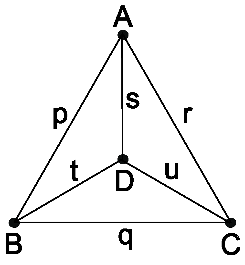
Example 5. 

Consider the graph $\Gamma =(V_{\Gamma },E_{\Gamma },{\psi }_{\Gamma })$ with vertex set $V_{\Gamma }=\{A,B,C,D\}$ and edge set $E_{\Gamma }=\{p=\{A,B\},q=\{B,C\},r=\{C,D\},s=\{A,D\}$, $t=\{B,D\}\}$ (see Figure 1). Its automorphism group $\mathrm{Aut}\left(V_{\Gamma }\right)$ is given by

$$\mathrm{Aut}\left(V_{\Gamma }\right)=\{{\mathrm{id}}_{{\mathbb{N}}_4},(A,C),(B,D),(A,C)(B,D)\}.$$

(16)

Let $G=\{{\mathrm{id}}_{{\mathbb{N}}_4},\delta =(B,D)\}$, and ${\Phi }_{V_{\Gamma }}$ be the subspace of ${\mathbb{R}}^4$ given by

$${\Phi }_{V_{\Gamma }}:=\{\phi =({\phi }^1,{\phi }^2,{\phi }^3,{\phi }^4)\in {\mathbb{R}}^4\mid {\phi }^1-{\phi }^3=0\}.$$

(17)

Clearly, $\phi \circ \delta =({\phi }^1,{\phi }^4,{\phi }^3,{\phi }^2)\in {\Phi }_{V_{\Gamma }}$ for all $\phi \in {\Phi }_{V_{\Gamma }}$; so, $({\Phi }_{V_{\Gamma }},G)$ is a $\mathrm{vw}$-graph perception pair for Γ.

The next example shows that we can have different perception pairs with the same graph and the same group.

Example 6. 

Let G be as in Example 5 and

$${\Phi }_{V_{\Gamma }}=\{\phi =({\phi }^1,{\phi }^2,{\phi }^3,{\phi }^4)\in {\mathbb{R}}^4\mid \sum _{i\in {\mathbb{N}}_4}{\left({\phi }^i\right)}^2\le 1\}.$$

(18)

Then $({\Phi }_{V_{\Gamma }},G)$ is a $\mathrm{vw}$-graph perception pair.

We can now define a simple class of GENEOs.

Example 7. 

Let $({\Phi }_{V_{\Gamma }},G)$ be as in Example 5 and a map F be defined by

$$F\left(\phi \right)=({\phi }^1/d_1,{\phi }^2/d_2,{\phi }^3/d_3,{\phi }^4/d_4),\phi \in {\Phi }_{V_{\Gamma }},\mathrm{and}{d}_1,d_2,d_3,d_4\in [1,\infty ).$$

(19)

If, for all $\phi =({\phi }^1,{\phi }^2,{\phi }^3,{\phi }^4)\in {\Phi }_{V_{\Gamma }}$ and $g\in G$, we have $F(\phi \circ g)=F\left(\phi \right)\circ g$, then

$$\left(\frac{{\phi }^1}{d_1},\frac{{\phi }^4}{d_2},\frac{{\phi }^3}{d_3},\frac{{\phi }^2}{d_4}\right)=\left(\frac{{\phi }^1}{d_1},\frac{{\phi }^4}{d_4},\frac{{\phi }^3}{d_3},\frac{{\phi }^2}{d_2}\right)$$

(20)

whence $d_2=d_4$; and the requirement that $F\left(\phi \right)\in {\Phi }_{V_{\Gamma }}$ entails $d_1=d_3$. Moreover, because of the nature of the $L^{\infty }$ norm,

$$\parallel F\left({\phi }_1\right)-F\left({\phi }_2\right){\parallel }_{\infty }\le \frac{1}{min\{d_1,d_2\}}\parallel {\phi }_1-{\phi }_2{\parallel }_{\infty }\le {\parallel {\phi }_1-{\phi }_2\parallel }_{\infty }$$

(21)

for all ${\phi }_1=({\phi }_1^1,{\phi }_1^2,{\phi }_1^3,{\phi }_1^4),{\phi }_2=({\phi }_2^1,{\phi }_2^2,{\phi }_2^3,{\phi }_2^4)\in {\Phi }_{V_{\Gamma }}$, whence F is non-expansive. Therefore, the map F defined above is a $\mathrm{vw}$-graph GENEO if and only if $d_1=d_3$ and $d_2=d_4$.

We now prepare for the first instances of graph permutants in Examples 10 and 11.

Example 8. 

Let $\Gamma =(V_{\Gamma },E_{\Gamma },{\psi }_{\Gamma })$ be the cycle graph $C_4$ with $V_{\Gamma }=\{A,B,C,D\}$. Its automorphism group is given by

$$\mathrm{Aut}\left(V_{\Gamma }\right)=\{{\mathrm{id}}_{{\mathbb{N}}_4},\alpha =(A,B,C,D),{\alpha }^2,{\alpha }^3,(A,C),(B,D),(A,B)(C,D),(A,D)(B,C)\}$$

(22)

and $G=\{{\mathrm{id}}_{{\mathbb{N}}_4},\alpha ,{\alpha }^2,{\alpha }^3\}$ is a subgroup of $\mathrm{Aut}\left(V_{\Gamma }\right)$.

If ${\Phi }_{V_{\Gamma }}$ is the same as in Example 5, then $({\Phi }_{V_{\Gamma }},G)$ is not a $\mathrm{vw}$-graph perception pair. However, if we define

$${\Phi }_{V_{\Gamma }}=\{\phi =({\phi }^1,{\phi }^2,{\phi }^3,{\phi }^4)\in {\mathbb{R}}^4\mid {\phi }^1+{\phi }^3=0={\phi }^2+{\phi }^4\}$$

(23)

then $({\Phi }_{V_{\Gamma }},\mathrm{Aut}\left(V_{\Gamma }\right))$, and, therefore, $({\Phi }_{V_{\Gamma }},G)$, are $\mathrm{vw}$-graph perception pairs.

Example 9. 

Let G be as in Example 8 and

$${\Phi }_{V_{\Gamma }}=\{\phi \in {\mathbb{R}}^4\mid {\parallel \phi \parallel }_{\infty }\le 1\}.$$

(24)

Then $({\Phi }_{V_{\Gamma }},G)$ is a $\mathrm{vw}$-graph perception pair.

Example 10. 

Let G be as in Example 8 and

$$H=\{h_1=(A,B)(C,D),h_2=(A,D)(B,C)\}\subseteq \mathrm{Aut}\left(V_{\Gamma }\right).$$

(25)

Then H is a $\mathrm{vw}$-graph permutant for $T={\mathrm{id}}_G$.

Example 11. 

Let Γ be as in Example 8 and

$$G=\{{\mathrm{id}}_{{\mathbb{N}}_4},{\alpha }^2,(A,B)(C,D),(A,D)(B,C)\}$$

(26)

be the Klein 4-group contained in $\mathrm{Aut}\left(V_{\Gamma }\right)$. If

$$H=\{(A,C),(B,D)\}\subseteq \mathrm{Aut}\left(V_{\Gamma }\right)$$

(27)

then H is a $\mathrm{vw}$-graph permutant for $T={\mathrm{id}}_G$.

As usual, in the following, we will denote by $K_n$ the complete graph on n vertices.

Proposition 4. 

Let $\Gamma :=K_n$ and $H\subseteq G=\mathrm{Aut}\left(V_{\Gamma }\right)\cong S_n$ be the set of all transpositions of $V_{\Gamma }$. Then H is a $\mathrm{vw}$-graph permutant for $T={\mathrm{id}}_G$.

Proof. 

Let $f\in H$ and $g\in G$; we show that $g\circ f\circ g^{-1}\in H$. Let us put $f:=(A,B)$ for some $A,B\in V_{\Gamma }$, $C:=g\left(A\right)$ and $D:=g\left(B\right)$. Then

$$g\circ f\circ g^{-1}\left(C\right)=g\circ f\left(A\right)=g\left(B\right)=D$$

(28)

$$g\circ f\circ g^{-1}\left(D\right)=g\circ f\left(B\right)=g\left(A\right)=C.$$

(29)

Take $L\in V_{\Gamma }$, different from both C and D; since g is bijective, $g^{-1}\left(L\right)\ne g^{-1}\left(C\right)=A$ and $g^{-1}\left(L\right)\ne g^{-1}\left(D\right)=B$. We thus have

$$g\circ f\circ g^{-1}\left(L\right)=g\circ g^{-1}\left(L\right)=L$$

(30)

whence $g\circ f\circ g^{-1}=(C,D)\in H$, as required. □

As stated in Theorem 1—which holds also in the graph-theoretical context, having a purely set-theoretical proof—the concept of a $\mathrm{vw}$-graph permutant can be used to define $\mathrm{vw}$-graph GENEOs.

Example 12. 

Let $({\Phi }_{V_{\Gamma }},G)$ be the same as in Example 9 and H be the same as in Example 10. Set $F\left(\phi \right)=\frac{1}{2}(\phi \circ h_1+\phi \circ h_2)$. Then $F\left({\Phi }_{V_{\Gamma }}\right)\subseteq {\Phi }_{V_{\Gamma }}$; therefore, by Theorem 1, F is a $\mathrm{vw}$-graph GENEO.

4.2. GENEOs on Graphs Weighted on Edges

The concepts of perception pairs, GEOs/GENEOs, and generalized permutants can be applied to $\mathrm{ew}$-graphs as well, as in Definitions 11, 12, and 13, respectively. Theorem 1 holds also in this case.

Definition 11. 

Let ${\Phi }_{E_{\Gamma }}$ be a set of functions from $E_{\Gamma }$ to $\mathbb{R}$ and G be a subgroup of $\mathrm{Aut}\left(E_{\Gamma }\right)$. If $({\Phi }_{E_{\Gamma }},G)$ is a perception pair, we will call it an $\mathrm{ew}$-graph perception pair for $\Gamma =(V_{\Gamma },E_{\Gamma },{\psi }_{\Gamma })$, and will write $\mathrm{dom}\left({\Phi }_{E_{\Gamma }}\right)=E_{\Gamma }$.

Definition 12. 

Let $({\Phi }_{E_{{\Gamma }_1}},G_1)$ and $({\Phi }_{E_{{\Gamma }_2}},G_2)$ be two $\mathrm{ew}$-graph perception pairs and $T:G_1\to G_2$ be a group homomorphism. If $F:{\Phi }_{E_{{\Gamma }_1}}\to {\Phi }_{E_{{\Gamma }_2}}$ is a GEO (resp. GENEO) from $({\Phi }_{E_{{\Gamma }_1}},G_1)$ to $({\Phi }_{E_{{\Gamma }_2}},G_2)$ with respect to T, we will say that F is an $\mathrm{ew}$-graph GEO (resp. $\mathrm{ew}$-graph GENEO).

Definition 13. 

Let $({\Phi }_{E_{{\Gamma }_1}},G_1)$ and $({\Phi }_{E_{{\Gamma }_2}},G_2)$ be two $\mathrm{ew}$-graph perception pairs and $T:G_1\to G_2$ be a group homomorphism. We say that $H\subseteq {E_{{\Gamma }_1}}^{E_{{\Gamma }_2}}$ is an $\mathrm{ew}$-graph permutant for T if ${\alpha }_g\left(H\right)\subseteq H$ for every $g\in G_1$; that is, ${\alpha }_g\left(f\right)=g\circ f\circ T\left(g^{-1}\right)\in H$ for every $f\in H$ and $g\in G_1$.

The group $\mathrm{Aut}(\Gamma )$ of all graph automorphisms of a graph $\Gamma$ induces a particular subgroup $\mathrm{Aut}\left(E_{\Gamma }\right)$ of the group $S_m$ of all permutations of $E_{\Gamma }$. The elements of $\mathrm{Aut}\left(E_{\Gamma }\right)$ can be considered to be those permutations of $E_{\Gamma }$ that directly correspond to the permutations of $V_{\Gamma }$ defining all graph automorphisms of $\Gamma$.

If $\Gamma =K_n$, the complete graph with n vertices, the group $\mathrm{Aut}(\Gamma )$ is isomorphic to $S_n$, and we have

$$S_n\cong \mathrm{Aut}\left(V_{\Gamma }\right)\cong \mathrm{Aut}\left(E_{\Gamma }\right)\subseteq S_m.$$

(31)

Therefore, we will consider $\mathrm{Aut}(\Gamma )$ and $\mathrm{Aut}\left(E_{\Gamma }\right)$ to be the same in this case.

Let us consider some examples of perception pairs and GENEOs in the context of $\mathrm{ew}$-graphs. Complete graphs are of particular interest because every simple graph with n vertices is a subgraph of $K_n$ and so can be identified by a map from the edge set of $K_n$ to $\{0,1\}$ (Section 5.1).

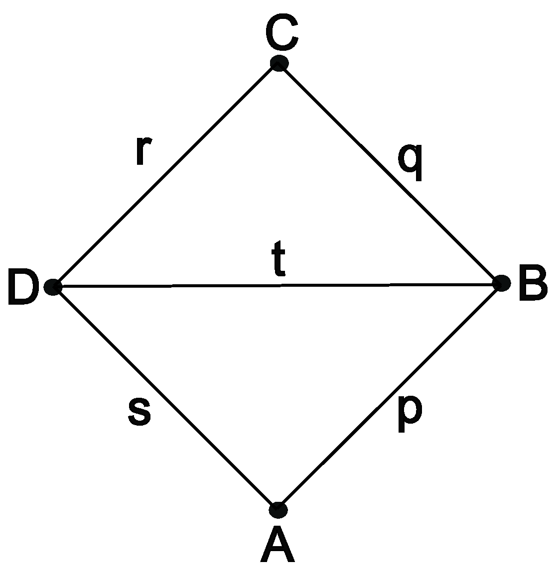
Example 13. 

Let $\Gamma =K_4=(V_{\Gamma },E_{\Gamma },{\psi }_{\Gamma })$ with $V_{K_4}=\{A,B,C,D\}$, and $E_{K_4}=\left\{p=\{A,B\},q=\{B,C\},r=\{A,C\},s=\{A,D\},t=\{B,D\},u=\{C,D\}\right\}$ (see Figure 2), and consider the group $G=\{{\mathrm{id}}_{E_{\Gamma }},\delta =\left(rs\right)\left(qt\right)\}\subseteq \mathrm{Aut}\left(E_{\Gamma }\right)$ together with the space ${\Phi }_{E_{\Gamma }}=\{\phi =({\phi }^1,{\phi }^2,{\phi }^3,{\phi }^4,{\phi }^5,{\phi }^6)\mid {\phi }^1+{\phi }^6=0\}\subseteq {\mathbb{R}}^m$ of the functions with opposite values on the two edges fixed by the elements of G. Clearly, $\phi \circ \delta \in {\Phi }_{E_{\Gamma }}$, and $({\Phi }_{E_{\Gamma }},G)$ is an $\mathrm{ew}$-graph perception pair.

Example 14. 

Let $({\Phi }_{E_{\Gamma }},G)$ be as in Example 13 and consider the map F defined by

$$\begin{array}{cc}\hfill F\left(\phi \right):=& ({\phi }^1/d_1,{\phi }^2/d_2,{\phi }^3/d_3,{\phi }^4/d_4,{\phi }^5/d_5,{\phi }^6/d_6),\hfill \\ \hfill & \phi \in {\Phi }_{E_{\Gamma }},\mathit{and}{d}_i\ge 1,\forall i\in {\mathbb{N}}_6.\hfill \end{array}$$

(32)

In order that $F\left(\phi \right)\in {\Phi }_{E_{\Gamma }}$, we should have $d_1=d_6$, and the requirement that F be equivariant with respect to G entails $d_3=d_4$ and $d_2=d_5$.

Moreover, a simple computation shows that

$$\begin{array}{cc}\hfill \parallel F\left({\phi }_1\right)-F\left({\phi }_2\right){\parallel }_{\infty }& \le \frac{1}{min\{d_1,d_2,d_3\}}{\parallel {\phi }_1-{\phi }_2\parallel }_{\infty }\hfill \\ & \le \parallel {\phi }_1-{\phi }_2{\parallel }_{\infty }\hfill \end{array}$$

(33)

for all ${\phi }_1=({\phi }_1^i/i\in {\mathbb{N}}_6),{\phi }_2=({\phi }_2^i/i\in {\mathbb{N}}_6)\in {\Phi }_{E_{\Gamma }}$, whence F is non-expansive.

Therefore, the map F defined above is an $\mathrm{ew}$-graph GENEO if and only if $d_1=d_6$, $d_2=d_5$, and $d_3=d_4$.

5. Experiments

This section illustrates the model of Section 4.2 and shows how graph GENEOs allow one to extract useful information from graphs. This can be done by “smart forgetting” of differences, either by some sort of average, but keeping the same dimension of the space of functions (as in Section 5.1), or by dimension reduction (as in Section 5.2). It should be noted that these are not new findings or results comparable with competitors, but just suggestions, by toy examples, of the possible use of the new tools provided in this paper. In particular, Section 5.1 analyzes the information that is preserved by a certain permutant on isomorphism classes of graphs with four vertices. Section 5.2 counts all possible generalized permutants relative to a pair of cycle graphs.

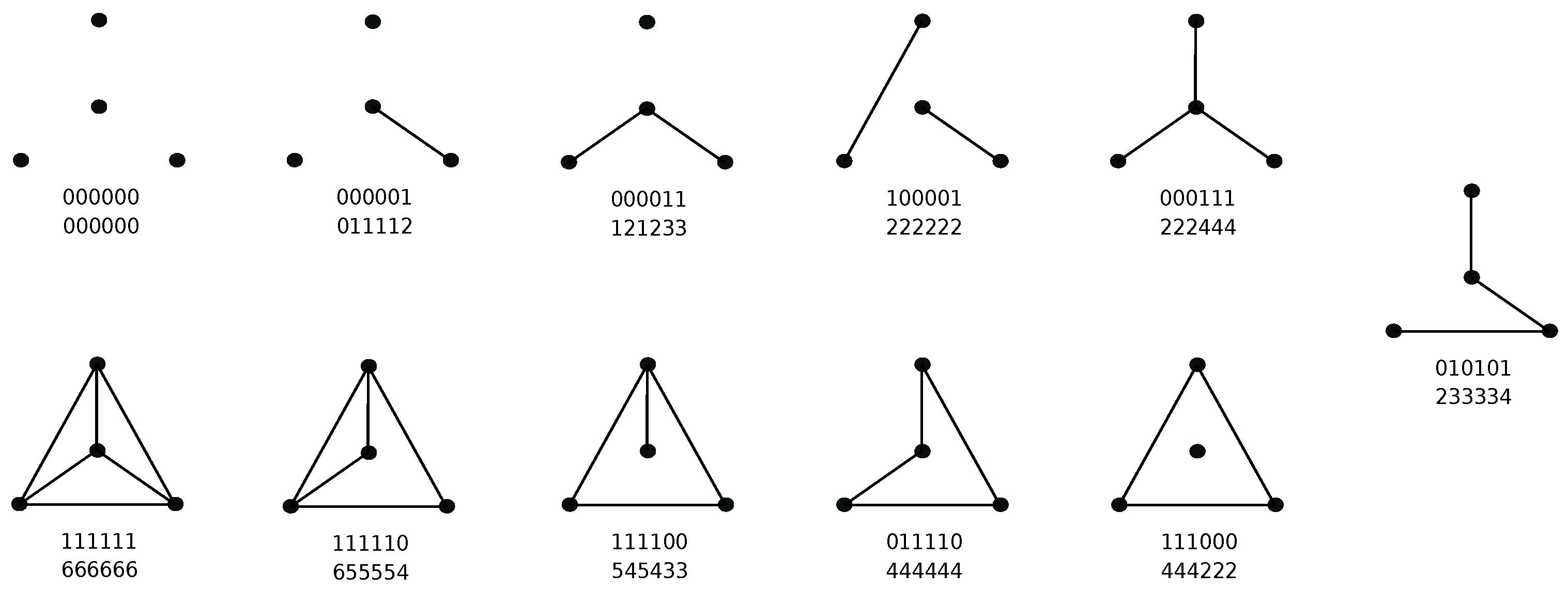
5.1. Subgraphs of $K_4$

The choice of a permutant determines how different functions are mapped to the same “signature” by the corresponding GENEO. In this subsection, we consider functions on the edge set of a complete graph $K_n$, taking values that are either 0 or 1; this means that each such function identifies a subgraph of $K_n$. A GENEO will, in general, produce functions that can have any real value, so no longer representing subgraphs. Intending to obtain equal results for “similar” subgraphs, we have chosen as a permutant the set of edge permutations produced by swapping two vertices in any possible way.

Let $\Gamma$ be the complete graph $K_4$ (Figure 2) with ${\Phi }_{E_{\Gamma }}:={\mathbb{R}}^6$. We have

$$S_4\cong \mathrm{Aut}\left(K_4\right)\cong \mathrm{Aut}\left(E_{K_4}\right)\subseteq S_6.$$

(34)

The subset $H:=\left\{\right(q,r\left)\right(s,t),(p,q\left)\right(s,u),(p,t\left)\right(r,u),(p,r\left)\right(t,u),(p,s\left)\right(q,u),(q,t\left)\right(r,s\left)\right\}$ of $G=\mathrm{Aut}\left(E_{K_4}\right)$ consisting of permutations of $E_{K_4}$ induced by all transpositions of $V_{K_4}$ is an $\mathrm{ew}$-graph permutant for $T={\mathrm{id}}_G$. Therefore, the operator $F:{\mathbb{R}}^6\to {\mathbb{R}}^6$ defined by

$$F\left(\phi \right):=\frac{1}{6}\sum _{h\in H}\phi \circ h$$

(35)

is an $\mathrm{ew}$-graph GENEO.

Subgraphs of $K_4$ can be represented by elements of

$${\Phi }_4:=\left\{\phi =({\phi }^1,\cdots ,{\phi }^6)\in {\Phi }_{E_{K_4}}\mid {\phi }^r\in \{0,1\},r\in {\mathbb{N}}_6\right\}$$

(36)

and the restriction $F_4$ of F to ${\Phi }_4\subseteq {\Phi }_{E_{K_4}}$ can be used to draw meaningful comparisons between them (see Figure 3). The following Definition 14 makes the discussion more fluid.

Definition 14. 

We say that the image $F_4\left(\phi \right)$ is an $F_4$-code for the subgraph $\phi \in {\Phi }_4$ of $K_4$. An $F_4$-code $c_1$ is said to be $F_4$-equivalent to an $F_4$-code $c_2$ (written $c_1{\sim }_4{c}_2$) if $c_2$ is the result of a permutation of $c_1$. The $F_4$-code ${\phi }^{{}^{\prime }}:=({\phi }^6,\cdots ,{\phi }^1)$ is called the reversal of $\phi :=({\phi }^1,\cdots ,{\phi }^6)\in {\Phi }_{E_{K_4}}$. Let ${\phi }_1,{\phi }_2\in {\Phi }_{E_{K_4}}$; we say that ${\phi }_1$ and ${\phi }_2$ are complementary if ${\phi }_1+{\phi }_2=(1,\cdots ,1)$.

Clearly, ${\sim }_4$ is an equivalence relation.

A simple program enabled us to compute all $F_4$-codes and to find that:

• Naturally enough, isomorphic subgraphs have $F_4$-equivalent codes. Therefore, in some cases, it suffices to consider only the 11 non-isomorphic subgraphs of $K_4$ (see Remark 1);
• Complementary subgraphs (i.e., subgraphs having vertex sets coinciding with $V_{K_4}$ and edge sets forming a partition of $E_{K_4}$) have complementary codes;
• There is only one case, up to graph isomorphisms, in which non-isomorphic subgraphs of $K_4$ have $F_4$-equivalent codes: ${\phi }_1=(1,1,1,0,0,0)$ and ${\phi }_2=(0,0,0,1,1,1)$ with $F_4\left({\phi }_1\right)=(4,4,4,2,2,2)/6$ and $F_4\left({\phi }_2\right)=(2,2,2,4,4,4)/6$. In this case, the graphs are complementary as well, which explains why we have equivalent codes despite the graphs being non-isomorphic. Moreover, ${\phi }_1$ and ${\phi }_2$ are reversals of each other, and so are the corresponding codes;
• If ${\phi }_1\in {\Phi }_4$ is a reversal of ${\phi }_2\in {\Phi }_4$, then $F_4\left({\phi }_1\right)$ is a reversal of $F_4\left({\phi }_2\right)$.

Remark 1. 

For example, the third graph of the upper row in Figure 3 consists of the two adjacent edges t and u and is represented by ${\phi }_3=(0,0,0,0,1,1)$ with $F_4\left({\phi }_3\right)=(1,2,1,2,3,3)/6$. The isomorphic graph consisting of edges p and r (not shown) is represented by ${\phi }_4=(1,0,1,0,0,0)$, with $F_4\left({\phi }_4\right)=(3,2,3,2,1,1)/6$. Their $F_4$-codes are $F_4$-equivalent, and are not $F_4$-equivalent to the $F_4$-code of a graph consisting of two non-adjacent edges—like the fourth in the upper row of Figure 3—although the representing 6-tuples obviously are permutations of each other.

It was also possible to compute $F_5$-codes for the 34 non-isomorphic subgraphs of $K_5$, and to find that they were never $F_5$-equivalent. A similar statement holds for the complete graph $K_3$.

5.2. Graph GENEOs for $C_6$ and $C_3$

All examples in Section 4.1, Section 4.2, and Section 5.1 were built on a single perception pair each. Still, the ground reason for using GENEOs is that of a “smart forgetting” of differences that are considered inessential. This can better be done by dimension reduction of the space of functions. This is where the use of two perception pairs comes into play. 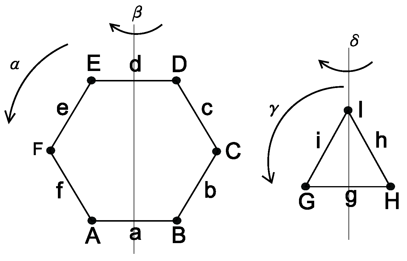This subsection is meant to illustrate the application of the generalized notion of permutants (Section 3) by mapping the edges of a small, auxiliary graph (the cyclic graph $C_3$) to the edges of the graph of interest (the cyclic graph $C_6$; see Figure 4). Note that we have great freedom, in that we are not bound to stick to graph homomorphisms: permutants are built as equivalence classes of maps from $E_{C_3}$ to $E_{C_6}$ that do not necessarily respect adjacencies.

Let $X:=(V_X,E_X,{\psi }_X)$ be the cycle graph $C_6$ (see Figure 4) with $V_X:=\{A,B,C,D,E,F\}$, $E_X:=\{a=\{A,B\},b=\{B,C\},c=\{C,D\},d=\{D,E\},e=\{E,F\},f=\{A,F\}\}$ and $Y:=(V_Y,E_Y,{\psi }_Y)$ be the cycle graph $C_3$ with $V_Y:=\{G,H,I\}$, $E_Y:=\{g=\{G,H\},h=\{H,I\},i=\{G,I\}\}.$

Their automorphisms groups, respectively, are the dihedral groups

$$D_6:=\{\alpha ,\beta \mid {\alpha }^6={\beta }^2={\left(\beta \alpha \right)}^2=1\},$$

(37)

$$D_3:=\{\gamma ,\delta \mid {\gamma }^3={\delta }^2={\left(\delta \gamma \right)}^2=1\},$$

(38)

where $\alpha :=(a,b,c,d,e,f),\beta :=(a,f)(b,e)(c,d),\gamma :=(g,h,i)$, and $\delta :=(g,i)$.

Let us put ${\Phi }_{E_X}:={\mathbb{R}}^6,{\Phi }_{E_Y}:={\mathbb{R}}^3$, and also put $G:=\mathrm{Aut}\left(E_X\right)=D_6$ and $K:=\mathrm{Aut}\left(E_Y\right)=D_3$, and consider the group homomorphism $T:G\to K$ given by $T\left(\alpha \right):=\gamma$ and $T\left(\beta \right):=\delta$.

There are 216 functions $p:E_Y\to E_X$ and the equivalence class of each (in the sense of Definition 5) is an $\mathrm{ew}$-graph permutant $H_p$ (Section 3.1). For the sake of conciseness, we will denote the function $p:=\{(g\mapsto e_1),(h\mapsto e_2),(i\mapsto e_3)\}$ simply by $p:={\mathrm{e}}_1{\mathrm{e}}_2{\mathrm{e}}_3$. For example, $p:=\left\{\right(g\mapsto c),(h\mapsto a),(i\mapsto f\left)\right\}$ will be written as $p:=\mathrm{caf}$.

The $\mathrm{ew}$-graph permutants $H_p$ with $p\in E_X^{E_Y}$ are of four possible sizes:

• There is only one $\mathrm{ew}$-graph permutant with two elements. It corresponds to the function $\mathrm{aec}$;
• There is only one $\mathrm{ew}$-graph permutant with four elements. It is induced by $\mathrm{bfd}$;
• There are five $\mathrm{ew}$-graph permutants with six elements each that correspond to the functions $\mathrm{aaa},\mathrm{abc},\mathrm{ace},\mathrm{add}$, and $\mathrm{afb}$;
• There are 15 $\mathrm{ew}$-graph permutants with 12 elements each that correspond to the functions $\mathrm{aab}$, $\mathrm{aac}$, $\mathrm{aad}$, $\mathrm{aae}$, $\mathrm{aaf}$, $\mathrm{abd}$, $\mathrm{acb}$, $\mathrm{acd}$, $\mathrm{adb}$, $\mathrm{adc}$, $\mathrm{baa}$, $\mathrm{bad}$, $\mathrm{bca}$, $\mathrm{bce}$, and $\mathrm{bdb}$.

Considering only the weights in $\{0,1\}$, it was possible to compute the $\mathrm{ew}$-graph GENEOs corresponding to the functions $\mathrm{aec}$ and $\mathrm{bfd}$. Similar computations can be made for the rest of the functions listed above. This detailed analysis of particular functions raised several questions and conjectures that we plan to study in the near future.

6. Discussion

This research aimed at extending the existing theory of Group Equivariant Non-Expansive Operators (GENEOs) in two directions:

• A general definition of permutant as a tool for producing GENEOs between two perception pairs (Theorem 1), while the original definition was limited to a single perception pair;
• The adaptation of the theory to graphs with a weight function defined either on vertices (Section 4.1) or on edges (Section 4.2).

Since every simple graph with n vertices can be identified with an edge-weighted subgraph of the complete graph $K_n$, where the weight function has $\{0,1\}$ as a range, permutants and GENEOs were used to analyze the set of subgraphs of $K_4$ (Section 5.1). A simple example of the construction of generalized permutants on graphs was also produced (Section 5.2).

An evident limitation of the presented GENEOs and permutants is that they are not aimed at particular graph-theoretical problems; they are just first, simple examples.

Here is a list of open problems:

• Is every GENEO between two perception pairs realizable as a combination of GENEOs coming from (generalized) permutants or permutant measures?
• What are other interesting permutants on $K_n$?
• Are there permutants that can help determine subgraphs of a given graph, with specified properties (e.g., being connected, Eulerian, Hamiltonian, etc.)?
• Can permutants and GENEOs help in refining the search for isomorphic graphs?

Apart from tackling these problems, a natural goal is to apply GENEOs and permutants to concrete problems where data occur as weighted graphs.

The repository https://gitlab.com/patrizio.frosini/graph-geneos contains the C++ programs used here (accessed on 5 December 2023).