E2H Distance-Weighted Minimum Reference Set for Numerical and Categorical Mixture Data and a Bayesian Swap Feature Selection Algorithm

Abstract

Generally, when developing classification models using supervised learning methods (e.g., support vector machine, neural network, and decision tree), feature selection, as a pre-processing step, is essential to reduce calculation costs and improve the generalization scores. In this regard, the minimum reference set (MRS), which is a feature selection algorithm, can be used. The original MRS considers a feature subset as effective if it leads to the correct classification of all samples by using the 1-nearest neighbor algorithm based on small samples. However, the original MRS is only applicable to numerical features, and the distances between different classes cannot be considered. Therefore, herein, we propose a novel feature subset evaluation algorithm, referred to as the “E2H distance-weighted MRS,” which can be used for a mixture of numerical and categorical features and considers the distances between different classes in the evaluation. Moreover, a Bayesian swap feature selection algorithm, which is used to identify an effective feature subset, is also proposed. The effectiveness of the proposed methods is verified based on experiments conducted using artificially generated data comprising a mixture of numerical and categorical features.

1. Introduction

Generally, classification tasks are executed using supervised learning models, such as support vector machines, neural networks, and decision trees. However, the explicit use of the selected effectiveness features for classification is essential when developing classification models. This process is called feature selection, and it is known to reduce the calculation time and improve the estimation accuracy [1,2]. Therefore, several feature selection algorithms have been proposed in the field of machine learning; these include out-of-bag error [3], inter–intra class distance ratio [4,5], genetic algorithms [6,7], bagging [8,9], CART [10,11], Lasso [12,13], BoLasso [14], ReliefF [15,16], and atom search [17].

In this study, we consider the minimum reference set (MRS) [18], another feature selection algorithm, for developing a high-quality classification model. In the MRS, we select a feature subset ${\mathit{F}}^{\prime }$ from among the feature set $\mathit{F}$ and calculate the Euclidean distances for all the pairwise samples belonging to different classes. Next, we test the correct classification of all samples using the 1-nearest neighbor (1NN) algorithm based on paired samples with close distances. In this regard, if we achieve the correct classification of all samples using a small sample size, we regard the corresponding feature subsets as desirable. In other words, the sample size that leads to no classification error is considered as the evaluation value of the feature subset ${\mathit{F}}^{\prime }$. Additional details on the MRS can be found in [18]. We consider the MRS to be reliable because it has been adopted in previous studies for feature selection [19,20,21,22]. However, the MRS presents the following two limitations:

One of these limitations is represented as “Issue 1” in Figure 1. Here, (A1) and (A2) denote feature spaces with values $x_1$ and $x_2$, and the blue circle and red cross represent the observation samples of two different classes. In these cases, the correct classification of all samples can be achieved using 1NN, explicitly based on samples enclosed in the square box. Notably, large distances between different classes in a feature space are often desirable to achieve a high generalization score. Therefore, feature space (A2) is better than space (A1). However, the feature space evaluations of (A1) and (A2) are the same (i.e., six) when using the original MRS [18], even if the feature space (A2) is known to be desirable. We consider this an issue because the MRS is a method used for identifying a desirable feature subset for the classification problem.

The second issue is indicated as “Issue 2” in Figure 1. The figure presents a three-dimensional feature space consisting of two numerical features $x_1,x_2\in \mathbb{R}$ and a categorical feature $x_3\in \{⧫,♣,♠\}$. Here, when $x_3=⧫$, the samples are correctly classified by the numerical features $x_1$ and $x_2$. In certain cases, categorical features, such as $x_3$, are also effective for classification. However, the original MRS [18] can only evaluate numerical features because it is based on the Euclidean distance. Although we can transform the categorical values into numerical values via one-hot encoding, large categorical values often lead to an increase in the dimension number [23]. When the sample size and dimension number are a and r, respectively, the time complexity of the 1NN algorithm based on the brute-force search is $\mathcal{O}\left(ar\right)$ [24]. Moreover, although the k-d tree [25] is a fast algorithm, it is affected by dimensionality [26]. The number of dimensions r increases the computational time, despite the existence of an algorithm with a time complexity of $\mathcal{O}(rlogr+loga)$ [26]. Therefore, we consider that the application of one-hot encoding to categorical features is not desirable because it leads to an increase in the dimensionality.

Therefore, herein, we propose a novel feature subset evaluation algorithm, called the E2H distance-weighted MRS (E2H MRS), to address the two aforementioned issues. Here, “E2” and “H” denote the squared Euclidian distance and Hamming distance, respectively. Note that we can measure the distances between samples in a feature space comprising a mixture of numerical and categorical values by using the mixture distance “E2H.” Moreover, we propose a Bayesian swap feature selection algorithm (BS-FS) to identify a subset of desirable features for classification. In this paper, we will present details regarding the E2H MRS and BS-FS algorithms.

2. Proposed Method

Herein, we explain the mathematical representation of feature subset selection and the proposed methods. The used variables are summarized in Appendixes Appendix A.1 and Appendix A.2.

2.1. Mathematical Representation of Feature Subset Selection

Let us denote a set ${\mathit{F}}^{\mathrm{r}}$ consisting of $n^{\mathrm{r}}$ numerical features and a set ${\mathit{F}}^{\mathrm{c}}$ consisting of $n^{\mathrm{c}}$ categorical features as follows:

$$\begin{array}{c}\hfill \begin{array}{c}\hfill {\mathit{F}}^{\mathrm{r}}=\{f_1^{\mathrm{r}},\cdots ,f_{n^{\mathrm{r}}}^{\mathrm{r}}\},{\mathit{F}}^{\mathrm{c}}=\{f_1^{\mathrm{c}},\cdots ,f_{n^{\mathrm{c}}}^{\mathrm{c}}\}.\end{array}\end{array}$$

(1)

For instance, $f_1^{\mathrm{r}}=“\mathrm{age}”$, $f_2^{\mathrm{r}}=“\mathrm{height}”$, $f_1^{\mathrm{c}}=“\mathrm{male}\mathrm{or}\mathrm{female}”$, $f_2^{\mathrm{c}}=“\mathrm{blood}\mathrm{type}”$, and so on. As these features are known to mix, all features can be represented as

$$\begin{array}{c}\hfill \begin{array}{c}\hfill \mathit{F}={\mathit{F}}^{\mathrm{r}}\cup {\mathit{F}}^{\mathrm{c}},\left|\mathit{F}\right|=n,n=n^{\mathrm{r}}+n^{\mathrm{c}}.\end{array}\end{array}$$

(2)

The proposed algorithm determines a feature subset ${\mathit{F}}_{\mathrm{opt}.}^{\prime }$ consisting of m effective features from among the all features $\mathit{F}$ to estimate the class $z\in \{{\mathrm{z}}_0,{\mathrm{z}}_1\}$, that is,

$$\begin{array}{c}\hfill \begin{array}{c}\hfill {\mathit{F}}_{\mathrm{opt}.}^{\prime }\subset \mathit{F},\left|{\mathit{F}}_{\mathrm{opt}.}^{\prime }\right|=m,m\le n,\end{array}\end{array}$$

(3)

where

$$\begin{array}{c}\hfill \begin{array}{c}\hfill {\mathit{F}}_{\mathrm{opt}.}^{\prime }=\underset{{\mathit{F}}^{\prime }\subset \mathit{F}}{\mathrm{argmin}}L\left({\mathit{F}}^{\prime }\right),\mathrm{s}.\mathrm{t}.,\left|{\mathit{F}}^{\prime }\right|=m.\end{array}\end{array}$$

(4)

Notably, the E2H MRS adopts a function L for evaluating the feature subset ${\mathit{F}}^{\prime }$. Because the feature subset ${\mathit{F}}^{\prime }$ consists of a mixture of numerical and categorical features, let us denote the feature vector of class $z\in \{{\mathrm{z}}_0,{\mathrm{z}}_1\}$ as

$$\begin{array}{c}\hfill \begin{array}{c}\hfill {\mathit{x}}^z={\left[{\mathit{x}}^{z,\mathrm{r}}{\mathit{x}}^{z,\mathrm{c}}\right]}^{\top },\end{array}\end{array}$$

(5)

where

$$\begin{array}{c}\hfill \begin{array}{cc}\hfill & {\mathit{x}}^{z,\mathrm{r}}={[x_1^{z,\mathrm{r}}\cdots x_{p^{\mathrm{r}}}^{z,\mathrm{r}}]}^{\top },\hfill \\ \hfill & {\mathit{x}}^{z,\mathrm{c}}={[x_1^{z,\mathrm{c}}\cdots x_{p^{\mathrm{c}}}^{z,\mathrm{c}}]}^{\top },\hfill \\ \hfill & p^{\mathrm{r}}+p^{\mathrm{c}}=m.\hfill \end{array}\end{array}$$

(6)

Here, ${\mathit{x}}^{z,\mathrm{r}}$ is a vector consisting of $p^{\mathrm{r}}$ numerical features, and ${\mathit{x}}^{z,\mathrm{c}}$ is a vector consisting of $p^{\mathrm{c}}$ categorical features. As examples, we use four features of “Sex”, “Embarked (Port of Embarkation)”, “Age”, “Fare” for Titanic survival prediction [27,28]. In this case, the features subset is ${\mathit{F}}^{\prime }=\{“\mathrm{Age}”,“\mathrm{Fare}”,“\mathrm{Sex}”,“\mathrm{Embarked}”\}\subset \mathit{F}$. $p^{\mathrm{r}}=2$, $p^{\mathrm{c}}=2$, and $m=4$ because “Age” and “Fare” are numerical features, “Sex” and “Embarked” are categorical features. Moreover, feature vector ${\mathit{x}}^z$ consists of these values.

When the feature vector ${\mathit{x}}^z$ consists of only categorical or numerical features, $(p^{\mathrm{c}},p^{\mathrm{r}})=(m,0)$ or $(p^{\mathrm{c}},p^{\mathrm{r}})=(0,m)$ is satisfied. The feature vector of the i-th observation sample is defined as ${\mathit{x}}_i^z$.

2.2. E2H Distance-Weighted MRS Algorithm

The E2H MRS algorithm developed for evaluating the feature subset ${\mathit{F}}^{\prime }$ is summarized in Algorithm 1. This algorithm outputs an evaluation $L\left({\mathit{F}}^{\prime }\right)$ by inputting the feature subset ${\mathit{F}}^{\prime }$. After initialization, all pairwise distances $D({\mathit{x}}^{{\mathrm{z}}_0},{\mathit{x}}^{{\mathrm{z}}_1};\gamma )$ between the classes ${\mathrm{z}}_0$ and ${\mathrm{z}}_1$ are computed (line 5). Next, the distance set $\mathbf{D}=\{d_1,d_2,\cdots \}$ is sorted by $D({\mathit{x}}^{{\mathrm{z}}_0},{\mathit{x}}^{{\mathrm{z}}_1};\gamma )$ (line 6). Although these processes are also included in the original MRS [18], only numerical features can be evaluated because the original MRS is based on the Euclidean distance. Therefore, we use another distance function to apply the MRS to the feature subset ${\mathit{F}}^{\prime }$ comprising a mixture of numerical and categorical features. The definitions of $D({\mathit{x}}^{{\mathrm{z}}_0},{\mathit{x}}^{{\mathrm{z}}_1};\gamma )$ will be explained in Section 2.3.

Algorithm 1 E2H MRS feature evaluation algorithm

Input:  Feature subset ${\mathit{F}}^{\prime }$, Hamming weight $\gamma$, distance weight $\delta$ Output:  Evaluation of the feature subset $L\left({\mathit{F}}^{\prime }\right)$ 1: Standardizing numerical features in ${\mathit{F}}^{\prime }$ on a value range of zero to one 2: Set initial data $\mathit{I}\leftarrow \varphi$, i.e., empty set 3: Set initial average distance $C\left(\mathit{I}\right)\leftarrow 0$ 4: Set initial classification error of all data based on 1-NN using $\mathit{I}$, $E\left(\mathit{I}\right)\leftarrow \infty$ 5: Calculating all pairwise distances $D({\mathit{x}}^{{\mathrm{z}}_0},{\mathit{x}}^{{\mathrm{z}}_1};\gamma )$ between different classes 6: Set $\mathbf{D}\leftarrow \{d_1,d_2,\cdots \}$ sorted by the smallest to largest distance on $D({\mathit{x}}^{{\mathrm{z}}_0},{\mathit{x}}^{{\mathrm{z}}_1};\gamma )$ 7: $k\leftarrow 1$ 8: while $E\left(\mathit{I}\right)\ne 0$ do 9:    Identify different class samples i and j related to $D({\mathit{x}}_i^{{\mathrm{z}}_0},{\mathit{x}}_j^{{\mathrm{z}}_1};\gamma )=d_k$ 10:    if $\{i,j\}\neg \subset \mathit{I}$ then 11:      Updating sample set $\mathit{I}\leftarrow \mathit{I}\cup \{i,j\}$ 12:      Updating distance $C\left(\mathit{I}\right)\leftarrow C\left(\mathit{I}\right)+d_k$ 13:    end if 14:    $k\leftarrow k+1$ 15: end while 16: Averaging distance $C\left(\mathit{I}\right)\leftarrow C\left(\mathit{I}\right)/\left|\mathit{I}\right|$ 17: Scoring $S(\mathit{I};\delta )\leftarrow {(1-C\left(\mathit{I}\right))}^{\delta }\left|\mathit{I}\right|$ 18: $L\left({\mathit{F}}^{\prime }\right)\leftarrow S(\mathit{I};\delta )$ 19: return  $L\left({\mathit{F}}^{\prime }\right)$

Next, two samples $\{i,j\}$ of different classes that are nearest to each other (i.e., $d_1$) are added to the set $\mathit{I}$. We then test $E\left(\mathit{I}\right)$, which denotes the classification error resulting from the 1NN algorithm based on the set $\mathit{I}$. The proposed distance function is used in the 1NN algorithm because the feature subset consists of a mixture of numerical and categorical features. If the error rate is not zero, that is, $E\left(\mathit{I}\right)\ne 0$, paired samples $\{i,j\}$ related to $d_2$ are added to $\mathit{I}$, and the error rate $E\left(\mathit{I}\right)$ is rechecked. Note that the evaluation value of the feature subset ${\mathit{F}}^{\prime }$ is calculated when the error rate is zero, that is, $E\left(\mathit{I}\right)=0$. The computation of the evaluation value in the original MRS [18] uses $\left|\mathit{I}\right|$, which is the size of the set $\mathit{I}$. This implies that the larger the sample size, the better the evaluation of feature subsets by the original MRS. However, although this method is valid, the distances between different classes are not considered. To consider the distances between different classes, we propose a novel feature subset evaluation function $S(\mathit{I};\delta )$ using $C\left(\mathit{I}\right)$, the average distance of $d_k$, which is obtained in the growth process of the set $\mathit{I}$. The evaluation value of the feature subset $L\left({\mathit{F}}^{\prime }\right)$ is obtained using these processes. Details pertaining to $S(\mathit{I};\delta )$ are explained in Section 2.4.

2.3. Distance Function

Let us now denote the distance between ${\mathit{x}}^{{\mathrm{z}}_0}$ and ${\mathit{x}}^{{\mathrm{z}}_1}$, consisting of a mixture of numerical and categorical values, as

$$\begin{array}{c}\hfill \begin{array}{c}\hfill D({\mathit{x}}^{{\mathrm{z}}_0},{\mathit{x}}^{{\mathrm{z}}_1};\gamma )=\frac{1}{p^{\mathrm{r}}+\gamma p^{\mathrm{c}}}\left(D^{\mathrm{E}2}({\mathit{x}}^{{\mathrm{z}}_0,\mathrm{r}},{\mathit{x}}^{{\mathrm{z}}_1,\mathrm{r}})+\gamma D^{\mathrm{H}}({\mathit{x}}^{{\mathrm{z}}_0,\mathrm{c}},{\mathit{x}}^{{\mathrm{z}}_1,\mathrm{c}})\right),\gamma \ge 0.\end{array}\end{array}$$

(7)

The first and second terms represent the squared Euclidean distance and the Hamming distance, respectively, that is,

$$\begin{array}{c}\hfill \begin{array}{cc}\hfill D^{\mathrm{E}2}({\mathit{x}}^{{\mathrm{z}}_0,\mathrm{r}},{\mathit{x}}^{{\mathrm{z}}_1,\mathrm{r}})& ={({\mathit{x}}^{{\mathrm{z}}_0,\mathrm{r}}-{\mathit{x}}^{{\mathrm{z}}_1,\mathrm{r}})}^{\top }({\mathit{x}}^{{\mathrm{z}}_0,\mathrm{r}}-{\mathit{x}}^{{\mathrm{z}}_1,\mathrm{r}})\hfill \\ \hfill & ={\displaystyle \sum _{i=1}^{p^{\mathrm{r}}}}{(x_i^{{\mathrm{z}}_0,\mathrm{r}}-x_i^{{\mathrm{z}}_1,\mathrm{r}})}^2,\hfill \end{array}\end{array}$$

(8)

$$D^{\mathrm{H}}({\mathit{x}}^{{\mathrm{z}}_0,\mathrm{c}},{\mathit{x}}^{{\mathrm{z}}_1,\mathrm{c}})={\displaystyle \sum _{i=1}^{p^{\mathrm{c}}}}\sigma (x_i^{{\mathrm{z}}_0,\mathrm{c}},x_i^{{\mathrm{z}}_1,\mathrm{c}}),$$

(9)

where

$$\begin{array}{c}\hfill \begin{array}{c}\hfill \sigma (x_i^{{\mathrm{z}}_0,\mathrm{c}},x_i^{{\mathrm{z}}_1,\mathrm{c}})=\left\{\begin{array}{cc}0,\hfill & x_i^{{\mathrm{z}}_0,\mathrm{c}}=x_i^{{\mathrm{z}}_1,\mathrm{c}}\hfill \\ 1,\hfill & x_i^{{\mathrm{z}}_0,\mathrm{c}}\ne x_i^{{\mathrm{z}}_1,\mathrm{c}}\hfill \end{array}\right..\end{array}\end{array}$$

(10)

In general, the Hamming distance is defined as the minimum number of substitutions required to change one string into another. In other words, it is the number of mismatches between two strings. Therefore, when regarding the $p^{\mathrm{c}}$-dimensional categorical features vector as a string of length $p^{\mathrm{c}}$, the number of mismatches between the categorical features vectors of two different classes can be represented by the Hamming distance. This number is calculated with Equations (9) and (10).

Moreover, we refer to $\gamma$ as the “Hamming weight” because it is a weight parameter used for categorical features. The parameter $\gamma$ is manually set by users, and when they have a hypothesis in which categorical features are important for classification, they set a large value. When we set $\gamma =0$, the effect of categorical features on distance disappears. The distance function defined by Equation (7) is similar to that used in the k-prototype algorithm [29].

The following theorem is satisfied for the proposed distance function $D({\mathit{x}}^{{\mathrm{z}}_0},{\mathit{x}}^{{\mathrm{z}}_1};\gamma )$:

Theorem 1. 

$$\begin{array}{c}\hfill \begin{array}{c}\hfill {\mathit{x}}^{z,\mathrm{r}}\in {[0,1]}^{p^{\mathrm{r}}}\Rightarrow D({\mathit{x}}^{{\mathrm{z}}_0},{\mathit{x}}^{{\mathrm{z}}_1};\gamma )\in [0,1].\end{array}\end{array}$$

Proof. 

$$\begin{array}{c}\hfill \begin{array}{cc}\hfill {\mathit{x}}^{z,\mathrm{r}}\in {[0,1]}^{p^{\mathrm{r}}}& \Rightarrow {\displaystyle \underset{{\mathit{x}}^{{\mathrm{z}}_0,\mathrm{r}},{\mathit{x}}^{{\mathrm{z}}_1,\mathrm{r}}}{max}}{D}^{\mathrm{E}2}({\mathit{x}}^{{\mathrm{z}}_0,\mathrm{r}},{\mathit{x}}^{{\mathrm{z}}_1,\mathrm{r}})=p^{\mathrm{r}}\hfill \\ & \Rightarrow {\displaystyle \underset{{\mathit{x}}^{{\mathrm{z}}_0},{\mathit{x}}^{{\mathrm{z}}_1}}{max}}\left[D^{\mathrm{E}2}({\mathit{x}}^{{\mathrm{z}}_0,\mathrm{r}},{\mathit{x}}^{{\mathrm{z}}_1,\mathrm{r}})+\gamma D^{\mathrm{H}}({\mathit{x}}^{{\mathrm{z}}_0,\mathrm{c}},{\mathit{x}}^{{\mathrm{z}}_1,\mathrm{c}})\right]=p^{\mathrm{r}}+\gamma p^{\mathrm{c}},\hfill \\ \hfill & \because {\displaystyle \underset{{\mathit{x}}^{{\mathrm{z}}_0,\mathrm{c}},{\mathit{x}}^{{\mathrm{z}}_1,\mathrm{c}}}{max}}{D}^{\mathrm{H}}({\mathit{x}}^{{\mathrm{z}}_0,\mathrm{c}},{\mathit{x}}^{{\mathrm{z}}_1,\mathrm{c}})=p^{\mathrm{c}}\hfill \\ \hfill & \Rightarrow {\displaystyle \underset{{\mathit{x}}^{{\mathrm{z}}_0},{\mathit{x}}^{{\mathrm{z}}_1}}{max}}D({\mathit{x}}^{{\mathrm{z}}_0},{\mathit{x}}^{{\mathrm{z}}_1};\gamma )=1\hfill \\ \hfill & \Rightarrow D({\mathit{x}}^{{\mathrm{z}}_0},{\mathit{x}}^{{\mathrm{z}}_1};\gamma )\in [0,1],\because {\displaystyle \underset{{\mathit{x}}^{{\mathrm{z}}_0},{\mathit{x}}^{{\mathrm{z}}_1}}{min}}\left[D^{\mathrm{E}2}({\mathit{x}}^{{\mathrm{z}}_0,\mathrm{r}},{\mathit{x}}^{{\mathrm{z}}_1,\mathrm{r}})+\gamma D^{\mathrm{H}}({\mathit{x}}^{{\mathrm{z}}_0,\mathrm{c}},{\mathit{x}}^{{\mathrm{z}}_1,\mathrm{c}})\right]=0\hfill \end{array}\end{array}$$

□

In other words, the range of $D({\mathit{x}}^{{\mathrm{z}}_0},{\mathit{x}}^{{\mathrm{z}}_1};\gamma )$ extends from zero to one when the condition ${\mathit{x}}^{z,\mathrm{r}}\in {[0,1]}^{p^{\mathrm{r}}}$ is satisfied. The process involved in the standardization of numerical features from zero to one is presented in line 1 of Algorithm 1.

2.4. Evaluation Function of a Feature Subset

Here, we explain the evaluation function $L\left({\mathit{F}}^{\prime }\right)$ of the feature subset ${\mathit{F}}^{\prime }$. In the original MRS [18], the sample size $\left|\mathit{I}\right|$ of set $\mathit{I}$ leading to the correct classification (no error) of all samples is adopted as an evaluation function of a feature subset. By including the distances between different classes in the original MRS, we propose

$$\begin{array}{c}\hfill \begin{array}{c}\hfill S(\mathit{I};\delta )={(1-C\left(\mathit{I}\right))}^{\delta }\left|\mathit{I}\right|,\delta \ge 0\end{array}\end{array}$$

(11)

as a novel feature subset evaluation function (line 17 in Algorithm 1). For the proposed evaluation function $S(\mathit{I};\delta )$, the following theorem is satisfied:

Theorem 2. 

$$\begin{array}{c}\hfill \begin{array}{c}\hfill {\mathit{x}}^{z,\mathrm{r}}\in {[0,1]}^{p^{\mathrm{r}}}\wedge \delta \ge 0\Rightarrow S(\mathit{I};\delta )\in [0,|\mathit{I}\left|\right].\end{array}\end{array}$$

Proof. 

$$\begin{array}{c}\hfill \begin{array}{cc}\hfill {\mathit{x}}^{z,\mathrm{r}}\in {[0,1]}^{p^{\mathrm{r}}}& \Rightarrow D({\mathit{x}}^{{\mathrm{z}}_0},{\mathit{x}}^{{\mathrm{z}}_1};\gamma )\in [0,1],\because \mathrm{Theorem}1\hfill \\ \hfill & \Rightarrow C\left(\mathit{I}\right)\in [0,1],\because C\left(\mathit{I}\right)\mathrm{is}\mathrm{average}\mathrm{of}D({\mathit{x}}^{{\mathrm{z}}_0},{\mathit{x}}^{{\mathrm{z}}_1};\gamma )\hfill \\ \hfill & \Rightarrow {(1-C\left(\mathit{I}\right))}^{\delta }\in [0,1],\because \delta \ge 0\hfill \\ \hfill & \Rightarrow S(\mathit{I};\delta )\in [0,|\mathit{I}\left|\right]\hfill \end{array}\end{array}$$

□

Note that the range of evaluation $S(\mathit{I};\delta )$ extends from zero to $\left|\mathit{I}\right|$ if the range of the numerical features ${\mathit{x}}^{z,\mathrm{r}}$ extends from zero to one. $C\left(\mathit{I}\right)$ is the average distance of set $\mathit{I}$ and is obtained using the different class distances $d_k$ represented in lines 12 and 16 of Algorithm 1. The range of $C\left(\mathit{I}\right)$ extends from zero to one because it denotes the average of $D({\mathit{x}}^{{\mathrm{z}}_0},{\mathit{x}}^{{\mathrm{z}}_1};\gamma )$ based on Theorem 1. Therefore, Theorem 2 is satisfied. Moreover, we understand that ${(1-C\left(\mathit{I}\right))}^{\delta }$ is a damping coefficient for $\left|\mathit{I}\right|$, based on Equation (11). $\delta$ is referred to as the “distance weight” because it is a parameter used for adjusting the damping coefficient based on the distance $C\left(\mathit{I}\right)$. In a typical classification problem, the distance between different classes in a features space should be long to decrease classification errors. In some works, feature spaces leading to a long distance between different classes were used for classification [30,31]. Therefore, we included the parameter $\delta$ to represent the weight of the distance between different classes in the proposed method. This parameter is manually set by the users. The distance between the different classes is emphasized when setting $\delta$ to a large value. In contrast, the sample size of set $\mathit{I}$ is emphasized when setting $\delta$ to a small value. The value of the proposed evaluation function $S(\mathit{I};\delta )$ approaches zero when the distance between different classes is large, and the sample size of $\mathit{I}$ is small. Notably, the smaller the value of $S(\mathit{I};\delta )$, the more effective the subset ${\mathit{F}}^{\prime }$; hence, we define

$$\begin{array}{c}\hfill \begin{array}{c}\hfill L\left({\mathit{F}}^{\prime }\right)=S(\mathit{I};\delta )\end{array}\end{array}$$

(12)

to evaluate ${\mathit{F}}^{\prime }$. This function is expressed in Equation (4).

Note that when setting $\delta =0$, the proposed evaluation function and the original MRS [18] have the same form, owing to

$$\begin{array}{c}\hfill \begin{array}{c}\hfill S(\mathit{I};\delta =0)=\left|\mathit{I}\right|.\end{array}\end{array}$$

(13)

In contrast, when setting $\delta \to \infty$, the evaluation value is

$$\begin{array}{c}\hfill \begin{array}{c}\hfill {\displaystyle \underset{\delta \to \infty }{lim}}S(\mathit{I};\delta )=\left\{\begin{array}{cc}0,\hfill & 0<C\left(\mathit{I}\right)\le 1\hfill \\ \left|\mathit{I}\right|,\hfill & C\left(\mathit{I}\right)=0\hfill \end{array}\right..\end{array}\end{array}$$

(14)

In most cases, $S(\mathit{I};\delta \to \infty )$ approaches zero because $C\left(\mathit{I}\right)=0$ (i.e., the average distance between classes ${\mathrm{z}}_0$ and ${\mathrm{z}}_1$ is zero) is not satisfied. This implies that when the distance weight $\delta$ is too large, the proposed evaluation function $S(\mathit{I};\delta )$ does not perform well.

2.5. Bayesian Swap Feature Selection Algorithm

In the brute-force search method, the number of calculations required to solve the optimization problem presented in Equation (4), that is, the number of calculations required for identifying a feature subset that minimizes $L\left({\mathit{F}}^{\prime }\right)$, is

$$\begin{array}{c}\hfill \begin{array}{c}\hfill T_{\mathrm{all}}(n,m)={}_n{\mathrm{C}}_m,\end{array}\end{array}$$

(15)

where n denotes the size of $\mathit{F}$, and m is the size of ${\mathit{F}}^{\prime }$. Therefore, when n is large, obtaining an optimal solution is difficult from the perspective of the calculation cost. In the original MRS [18], an approach for finding the approximate solution is adopted. In particular, the first process randomly chooses m features from among the all features $\mathit{F}$, and the second process gradually improves the evaluation value $L\left({\mathit{F}}^{\prime }\right)$ by swapping the features. Additional details on this method are explained in [18]. The number of calculations required when using this method is

$$\begin{array}{c}\hfill \begin{array}{c}\hfill T_{\mathrm{fsa}}(n,m)=m(n-m).\end{array}\end{array}$$

(16)

Thus, this algorithm significantly reduces the calculation cost compared to the brute-force search. However, the final adopted feature subset depends on the initially selected feature subset. Therefore, we adopt an approach using the initial feature subset obtained via Bayesian optimization. The Bayesian optimization algorithm is a tree-structured parzen estimator algorithm (TPE) [32], and it is used in the optimization framework “optuna” (v2.0.0) [33].

A feature selection algorithm based on the described approach is outlined in Algorithm 2. The input values comprise the all features of set $\mathit{F}$, the dimension number m, and the number of iterations in the Bayesian optimization b. The output is an approximate solution ${\mathit{F}}_{\mathrm{opt}.}^{*}.$ We represent $L\left({\mathit{F}}_{\mathrm{opt}.}^{*}\right)\simeq L\left({\mathit{F}}_{\mathrm{opt}.}^{\prime }\right)$ because $L\left({\mathit{F}}_{\mathrm{opt}.}^{*}\right)$ is expected to be close to $L\left({\mathit{F}}_{\mathrm{opt}.}^{\prime }\right)$, which is an evaluation of the optimal solution ${\mathit{F}}_{\mathrm{opt}.}^{\prime }.$

Algorithm 2 Bayesian swap feature subset selection algorithm (BS-FS)

Input:  Feature set $\mathit{F}$, feature dimension m, iterations of the Bayesian optimization b Output:  Approximation solution of the feature subset ${\mathit{F}}_{\mathrm{opt}.}^{*}$, i.e., $L\left({\mathit{F}}_{\mathrm{opt}.}^{*}\right)\simeq L\left({\mathit{F}}_{\mathrm{opt}.}^{\prime }\right)$ 1: for $t=1$ to b do 2:    Bayesian selection (TPE) of m features ${\mathit{F}}_t^{\prime }\leftarrow \{f_1,f_2,\cdots ,f_m\}\subset \mathit{F}$ 3:    Calculate $L\left({\mathit{F}}_t^{\prime }\right)$ 4: end for 5: Solve ${\mathit{F}}_{\mathrm{opt}.}^{*}\leftarrow \underset{{\mathit{F}}_t^{\prime }}{\mathrm{argmin}}\{L\left({\mathit{F}}_t^{\prime }\right)\mid t=1,\cdots ,b\}$, where ${\mathit{F}}_{\mathrm{opt}.}^{*}=\{f_1^{*},f_2^{*},\cdots ,f_m^{*}\}$ 6: Obtain the difference set ${\overline{\mathit{F}}}_{\mathrm{opt}.}^{*}\leftarrow \mathit{F}\setminus {\mathit{F}}_{\mathrm{opt}.}^{*}$, where ${\overline{\mathit{F}}}_{\mathrm{opt}.}^{*}=\{{\overline{f}}_1^{*},{\overline{f}}_2^{*},\cdots ,{\overline{f}}_{n-m}^{*}\}$ 7: for $i=1$ to m do 8:    for $j=1$ to $n-m$ do 9:      Swap $f_i^{*}$ and ${\overline{f}}_j^{*}$, i.e., ${\mathit{F}}_{\mathrm{opt}.}^{*,\mathrm{swap}}\leftarrow {\mathit{F}}_{\mathrm{opt}.}^{*}\setminus \left\{f_i^{*}\right\}\cup \left\{{\overline{f}}_j^{*}\right\}$, ${\overline{\mathit{F}}}_{\mathrm{opt}.}^{*,\mathrm{swap}}\leftarrow {\overline{\mathit{F}}}_{\mathrm{opt}.}^{*}\setminus \left\{{\overline{f}}_j^{*}\right\}\cup \left\{f_i^{*}\right\}$ 10:      if $L\left({\mathit{F}}_{\mathrm{opt}.}^{*,\mathrm{swap}}\right)<L\left({\mathit{F}}_{\mathrm{opt}.}^{*}\right)$ then 11:         Accept the swap, i.e., ${\mathit{F}}_{\mathrm{opt}.}^{*}\leftarrow {\mathit{F}}_{\mathrm{opt}.}^{*,\mathrm{swap}}$, ${\overline{\mathit{F}}}_{\mathrm{opt}.}^{*}\leftarrow {\overline{\mathit{F}}}_{\mathrm{opt}.}^{*,\mathrm{swap}}$ 12:      end if 13:    end for 14: end for 15: return ${\mathit{F}}_{\mathrm{opt}.}^{*}$

Note that lines 1–5 in Algorithm 2 detail the Bayesian optimization processes used for searching for the initial feature subset. We choose ${\mathit{F}}_t^{\prime }\subset \mathit{F}$ and determine its evaluation value, $L\left({\mathit{F}}_t^{\prime }\right)$. Note that t denotes the iteration ID of the Bayesian optimization. The relevant Bayesian optimization processes are repeated b times, and the feature subset of the minimum evaluation value is selected as the initial subset ${\mathit{F}}_{\mathrm{opt}.}^{*}$ (line 5). Subsequently, the evaluation value is improved by swapping each feature in the initial subset ${\mathit{F}}_{\mathrm{opt}.}^{*}$ and the remaining subset ${\overline{\mathit{F}}}_{\mathrm{opt}.}^{*}=\mathit{F}\setminus {\mathit{F}}_{\mathrm{opt}.}^{*}$. These processes are indicated in lines 6–14 of Algorithm 2. We refer to this algorithm as the “Bayesian swap feature selection algorithm (BS-FS)” because this method is a combination of Bayesian optimization and feature swapping.

Using Algorithm 2, the number of calculation evaluation functions in the BS-FS is

$$\begin{array}{c}\hfill \begin{array}{cc}\hfill T_{\mathrm{bs}}(n,m,b)& =b+m(n-m)\hfill \\ \hfill & =b+mn-m^2.\hfill \end{array}\end{array}$$

(17)

In general, $n,b\gg m$ is satisfied as a parameter relationship. Therefore, the time complexity of Algorithm 2 is $\mathcal{O}(b+n)$. This algorithm is fast compared to the brute-force search method. However, if the number of maximum iterations b is too large, the number of calculations for BS-FS is larger than that for the brute-force search method (i.e., $T_{\mathrm{bs}}(n,m,b)>T_{\mathrm{all}}(n,m)$). The boundary point $b^{\prime }$ is

$$\begin{array}{c}\hfill \begin{array}{c}\hfill b^{\prime }={}_n{\mathrm{C}}_m+m^2-mn\iff T_{\mathrm{bs}}(n,m,b^{\prime })=T_{\mathrm{all}}(n,m).\end{array}\end{array}$$

(18)

In other words, the number of maximum iterations for the Bayesian optimization, b, must be less than $b^{\prime }$.

3. Artificial Dataset for the Verification of the Proposed Methods

Further, we verified the effectiveness of the proposed methods using an artificial dataset. Note that the effective feature subset for classification is defined as

$$\begin{array}{c}\hfill \begin{array}{c}\hfill {\mathit{F}}^{\mathrm{Sol}.}=\{f_1^{\mathrm{Sol}.,\mathrm{r}},f_2^{\mathrm{Sol}.,\mathrm{r}},f_1^{\mathrm{Sol}.,\mathrm{c}},f_2^{\mathrm{Sol}.,\mathrm{c}}\},\end{array}\end{array}$$

(19)

where $\{f_1^{\mathrm{Sol}.,\mathrm{r}},f_2^{\mathrm{Sol}.,\mathrm{r}}\}\subset {\mathit{F}}^{\mathrm{r}}$, and $\{f_1^{\mathrm{Sol}.,\mathrm{c}},f_2^{\mathrm{Sol}.,\mathrm{c}},\}\subset {\mathit{F}}^{\mathrm{c}}$. In other words, the combination of two numeric features and two categorical features forms an effective feature subset for classification tasks. Let us denote the values of these features as $x_1$, $x_2$, $x_3$, and $x_4$. In particular, because $x_3$ and $x_4$ are categorical features,

$$\begin{array}{c}\hfill \begin{array}{c}\hfill x_3\in \{♣,♠\},x_4\in \{♢,♡\}.\end{array}\end{array}$$

(20)

Although we set a binary state as a categorical feature for simplification, because we adopted the Hamming distance $D^{\mathrm{H}}$, the number of states of a categorical feature can be any number of states. In this study, we generated the feature vectors $\mathit{x}={\left[x_1{x}_2{x}_3{x}_4\right]}^{\top }$ related to the feature subset ${\mathit{F}}^{\mathrm{Sol}.}$ based on the probability distribution. An overview of this is presented in Figure 2. The samples $x_1$ and $x_2$ of class ${\mathrm{z}}_0$ (blue circles) are generated based on a Gaussian distribution $\mathcal{N}$, defined as

$$\begin{array}{c}\hfill \begin{array}{c}\hfill f_{{\mathrm{z}}_0}(x_1,x_2;e^{\mathrm{c}})=\mathcal{N}(\mathit{u}\left(e^{\mathrm{c}}\right),\mathit{v}).\end{array}\end{array}$$

(21)

To determine the effects of categorical features, the mean vector $\mathit{u}$ is defined as follows:

$$\begin{array}{c}\hfill \begin{array}{c}\hfill \mathit{u}\left(e^{\mathrm{c}}\right)=\left\{\begin{array}{cc}{\left[u_1{u}_2\right]}^{\top },\hfill & (x_3,x_4)=(♣,♢)\hfill \\ [u_1+e^{\mathrm{c}}{u}_2{]}^{\top },\hfill & (x_3,x_4)=(♣,♡)\hfill \\ [u_1{u}_2+e^{\mathrm{c}}{]}^{\top },\hfill & (x_3,x_4)=(♠,♢)\hfill \\ [u_1-e^{\mathrm{c}}{u}_2-e^{\mathrm{c}}{]}^{\top },\hfill & (x_3,x_4)=(♠,♡)\hfill \end{array}\right..\end{array}\end{array}$$

(22)

This implies that the average vector is shifted by $e^{\mathrm{c}}$ depending on the categorical features. Only in the case of $(x_3,x_4)=(♠,♡)$, the average vector is shifted by $-e^{\mathrm{c}}$.

The samples $x_1$, $x_2$ of class ${\mathrm{z}}_1$ (red circles) are generated based on a Gaussian mixture distribution, defined as

$$\begin{array}{c}\hfill \begin{array}{c}\hfill f_{{\mathrm{z}}_1}(x_1,x_2;e^{\mathrm{c}},e^{\mathrm{r}})=\frac{1}{3}{\displaystyle \sum _{i=1}^3}\mathcal{N}({\mathit{u}}_i(e^{\mathrm{c}},e^{\mathrm{r}}),\mathit{v}).\end{array}\end{array}$$

(23)

To determine the effect of the categorical features, the mean vectors ${\mathit{u}}_1,{\mathit{u}}_2$, and ${\mathit{u}}_3$ are defined as

$$\begin{array}{c}\hfill \begin{array}{c}\hfill {\mathit{u}}_1(e^{\mathrm{c}},e^{\mathrm{r}})=\left\{\begin{array}{cc}{[u_1+e^{\mathrm{r}}{u}_2]}^{\top },\hfill & (x_3,x_4)=(♣,♢)\hfill \\ [u_1+e^{\mathrm{c}}+e^{\mathrm{r}}{u}_2{]}^{\top },\hfill & (x_3,x_4)=(♣,♡)\hfill \\ [u_1+e^{\mathrm{r}}{u}_2+e^{\mathrm{c}}{]}^{\top },\hfill & (x_3,x_4)=(♠,♢)\hfill \\ [u_1-e^{\mathrm{c}}+e^{\mathrm{r}}{u}_2-e^{\mathrm{c}}{]}^{\top },\hfill & (x_3,x_4)=(♠,♡)\hfill \end{array}\right.,\end{array}\end{array}$$

(24)

$$\begin{array}{c}\hfill \begin{array}{c}\hfill {\mathit{u}}_2(e^{\mathrm{c}},e^{\mathrm{r}})=\left\{\begin{array}{cc}{[u_1{u}_2+e^{\mathrm{r}}]}^{\top },\hfill & (x_3,x_4)=(♣,♢)\hfill \\ [u_1+e^{\mathrm{c}}{u}_2+e^{\mathrm{r}}{]}^{\top },\hfill & (x_3,x_4)=(♣,♡)\hfill \\ [u_1{u}_2+e^{\mathrm{c}}+e^{\mathrm{r}}{]}^{\top },\hfill & (x_3,x_4)=(♠,♢)\hfill \\ [u_1-e^{\mathrm{c}}{u}_2-e^{\mathrm{c}}+e^{\mathrm{r}}{]}^{\top },\hfill & (x_3,x_4)=(♠,♡)\hfill \end{array}\right.,\end{array}\end{array}$$

(25)

$$\begin{array}{c}\hfill \begin{array}{c}\hfill {\mathit{u}}_3(e^{\mathrm{c}},e^{\mathrm{r}})=\left\{\begin{array}{cc}{[u_1+e^{\mathrm{r}}{u}_2+e^{\mathrm{r}}]}^{\top },\hfill & (x_3,x_4)=(♣,♢)\hfill \\ [u_1+e^{\mathrm{c}}+e^{\mathrm{r}}{u}_2+e^{\mathrm{r}}{]}^{\top },\hfill & (x_3,x_4)=(♣,♡)\hfill \\ [u_1+e^{\mathrm{r}}{u}_2+e^{\mathrm{c}}+e^{\mathrm{r}}{]}^{\top },\hfill & (x_3,x_4)=(♠,♢)\hfill \\ [u_1-e^{\mathrm{c}}+e^{\mathrm{r}}{u}_2-e^{\mathrm{c}}+e^{\mathrm{r}}{]}^{\top },\hfill & (x_3,x_4)=(♠,♡)\hfill \end{array}\right..\end{array}\end{array}$$

(26)

In other words, the samples of class ${\mathrm{z}}_1$ are shifted by $e^{\mathrm{r}}$ compared with the samples of class ${\mathrm{z}}_0$. The variance–covariance matrix is defined as follows:

$$\begin{array}{c}\hfill \begin{array}{c}\hfill \mathit{v}=\left[\begin{array}{cc}v& 0\\ 0& v\end{array}\right].\end{array}\end{array}$$

(27)

The distribution has the following parameters: $e^{\mathrm{r}}$ and $e^{\mathrm{c}}$. For the artificial samples generated by the distribution based on large values of $e^{\mathrm{r}}$, the classification of two classes using the numerical features $x_1$ and $x_2$ is simple because the distances between different classes are large. For artificial samples generated by the distribution based on large values of $e^{\mathrm{c}}$, it is necessary to use the categorical features $x_3$ and $x_4$ for classification. Therefore, $e^{\mathrm{r}}$ represents a “numerical effect,” and $e^{\mathrm{c}}$ represents a “categorical effect.”

The generated feature spaces in four dimensions ($x_1,x_2\in \mathbb{R}$, $x_3,\in \{♣,♠\}$, $x_4\in \{♢,♡\}$) are presented in Figure 3: (A) $(e^{\mathrm{c}},e^{\mathrm{r}})=(10,30)$, (B) $(e^{\mathrm{c}},e^{\mathrm{r}})=(10,50)$, (C) $(e^{\mathrm{c}},e^{\mathrm{r}})=(30,30)$, and (D) $(e^{\mathrm{c}},e^{\mathrm{r}})=(30,50)$. The values of the categorical features $x_3$ and $x_4$ change from left to right. The rightmost figure depicts an explicit scatter plot of the numerical features $x_1$ and $x_2$, that is, it does not consider the categorical features $x_3$ and $x_4$. Comparing (A) and (B), we can establish that the distance between different classes increases for a large value of the numerical effect $e^{\mathrm{r}}$. Moreover, even if we do not consider the categorical features $x_3$ and $x_4$, we can classify the samples owing to the small value of the categorical effect $e^{\mathrm{c}}$. In contrast, (C) and (D) represent spaces with large categorical effects $e^{\mathrm{c}}$. In this case, we can observe that the categorical features $x_3$ and $x_4$ are required for correct classification. We can control the difficulty level of classification using the parameters $e^{\mathrm{r}}$ and $e^{\mathrm{c}}$. Therefore, the method for the generation of artificial data described in this section is appropriate for verifying the proposed algorithms. Note that the generated values of the numerical features $x_1$ and $x_2$ are standardized from zero to one to satisfy Theorems 1 and 2.

The numerical examples of feature spaces (A)–(D) calculated by Algorithm 1 and Equation (11) are provided in

Table 1. Evaluation scores of the feature spaces (A)–(D) shown in Figure 3. $(\gamma ,\delta )=(0,0)$ represents original MRS and $(\gamma ,\delta )=(1,1)$ and $(1,5)$ represent E2H MRS. Note that total samples size on each feature space is 120 (class ${\mathrm{z}}_0$: 60, class ${\mathrm{z}}_1:60$).

Feature Space $({\mathit{e}}^{\mathbf{c}},{\mathit{e}}^{\mathbf{r}})$	Setting Parameters $(\mathit{\gamma },\mathit{\delta })$ 1	MRS Size $\left|\mathit{I}\right|$	Damping Coefficient ${(1-\mathit{C}\left(\mathit{I}\right))}^{\mathit{\delta }}$	Score $\mathit{S}(\mathit{I};\mathit{\delta })$ 2
(A) $(10,30)$	(0, 0)	48	1.000	48.00
(B) $(10,50)$	(0, 0)	56	1.000	56.00
(C) $(30,30)$	(0, 0)	63	1.000	63.00
(D) $(30,50)$	(0, 0)	67	1.000	67.00
(A) $(10,30)$	(1, 1)	35	0.983	34.41
(B) $(10,50)$	(1, 1)	26	0.960	24.95
(C) $(30,30)$	(1, 1)	35	0.993	34.77
(D) $(30,50)$	(1, 1)	27	0.981	26.48
(A) $(10,30)$	(1, 5)	35	0.844	29.54
(B) $(10,50)$	(1, 5)	26	0.661	17.20
(C) $(30,30)$	(1, 5)	35	0.935	32.73
(D) $(30,50)$	(1, 5)	27	0.822	22.20

¹ $\gamma$: Hamming weight, $\delta$: distance weight. ² The lower the value of S (I; $\delta$), the better is the feature space for classification.

. $S(\mathit{I};\delta )$, $\left|\mathit{I}\right|$, and ${(1-C\left(\mathit{I}\right))}^{\delta }$ represent the evaluation value, the size of MRS, and the damping coefficient, respectively. These values are calculated using Algorithm 1 and Equation (11). Notably, the lower the value of $S(\mathit{I};\delta )$, the better the feature space is for classification. For Algorithm 1, we adopted $(\gamma ,\delta )\in \left\{\right(0,0),(1,1),(1,5\left)\right\}$ as the Hamming weight $\gamma$ and distance weight $\delta$. The parameters $\gamma$ and $\delta$ are manually set by the users. $(\gamma ,\delta )=(0,0)$ indicate the original MRS, and $(\gamma ,\delta )=(1,1)$ and $(1,5)$ represent the proposed method E2H MRS. In the case of $(\gamma ,\delta )=(0,0)$, although (B) and (D) are perceptually desirable feature spaces for classification, the best space based on evaluation value $S(\mathit{I};\delta )$ is (A). The method did not determine (D) as the best feature space. This can be attributed to the Hamming weight $\gamma =0$, i.e., the method did not consider the effect of the categorical feature values $x_3$ and $x_4$. Similarly, in the case of $(\gamma ,\delta )=(0,0)$, the score of (B) was worse than that of (A), which can be attributed to the distance weight $\delta =0$, i.e., it did not consider distance between different classes. In contrast, when adopting $(\gamma ,\delta )=(1,1)$, the proposed method determined (B) and (D) as desirable feature spaces for classification because the effects of categorical features and the distance between different classes are considered. Moreover, when adopting $(\gamma ,\delta )=(1,5)$, the effect of the damping coefficient on the evaluation value increased. Therefore, we consider the proposed method of E2H MRS to be better than original MRS method for evaluating features subset.

4. Experiment 1: Relationship between the Distance between Different Classes and the E2H MRS Evaluation

4.1. Objective and Outline

In the original MRS [18], the distance between different classes is not considered because the evaluation value of the feature subset is the sample size of the set $\mathit{I}$. Therefore, we propose a novel evaluation function $S(\mathit{I};\delta )$ that includes the distance and sample size. To verify its effectiveness, we generate a feature subset ${\mathit{F}}^{\prime },m=4$ comprising two numerical and two categorical features, and we calculate the evaluation value $S(\mathit{I};\delta )=L\left({\mathit{F}}^{\prime }\right)$.

Notably, we adopt $e^{\mathrm{r}}\in \{20,30,40,50\}$ and $e^{\mathrm{c}}=20$ as the parameters for generating artificial feature subsets. Moreover, $\delta \in \{0,1,2,3,4\}$ is adopted for the sensitivity analysis of the distance weight. When $\delta =0$, the evaluation functions of the original MRS [18] and E2H MRS have the same form. In other words, the results of $\delta \ge 1$ represent E2H MRS but not the original MRS. The number of generated samples is

$$\begin{array}{c}\hfill \begin{array}{c}\hfill (n_{{\mathrm{z}}_0},n_{{\mathrm{z}}_1})\in \{(12,12),(24,24),(48,48),(96,96),(192,192),(384,384)\},\end{array}\end{array}$$

(28)

where $n_z$ represents the samples of class $z\in \{{\mathrm{z}}_0,{\mathrm{z}}_1\}$. As stated, all numerical features are standardized from zero to one to satisfy Theorems 1 and 2. Moreover, we perform experiments using 100 random seeds to obtain stable results because the generated data depend on randomness.

4.2. Result and Discussion

The results obtained are summarized in Figure 4. The vertical axis represents the average evaluation value $S(\mathit{I};\delta )=L\left({\mathit{F}}^{\prime }\right)$ on 100 seeds. The horizontal axis represents the numerical effect, $e^{\mathrm{r}}$. In other words, the greater the value of $e^{\mathrm{r}}$, the greater the distance between different classes in the feature subset. The dashed line indicates the result of the original MRS ($\delta =0$), and the solid lines indicate the results of the E2H MRS ($\delta \ge 1$).

The greater the distance between different classes, the more effective the feature subset for classification. Therefore, when $e^{\mathrm{r}}$ is large, the evaluation value $L\left({\mathit{F}}^{\prime }\right)$ should ideally be small. From this viewpoint, the results of the original MRS ($\delta =0$) are deemed to be inappropriate when the sample size is greater than 48. This is because the original MRS cannot consider the distance between different classes. In contrast, in the case of the E2H MRS ($\delta \ge 1$), the evaluation values are small when the distance between different classes is large. Therefore, the E2H MRS is effective in identifying feature subsets with large distances between different classes.

5. Experiment 2: Effectiveness of BS-FS in Finding Desirable Feature Subsets

5.1. Objective and Outline

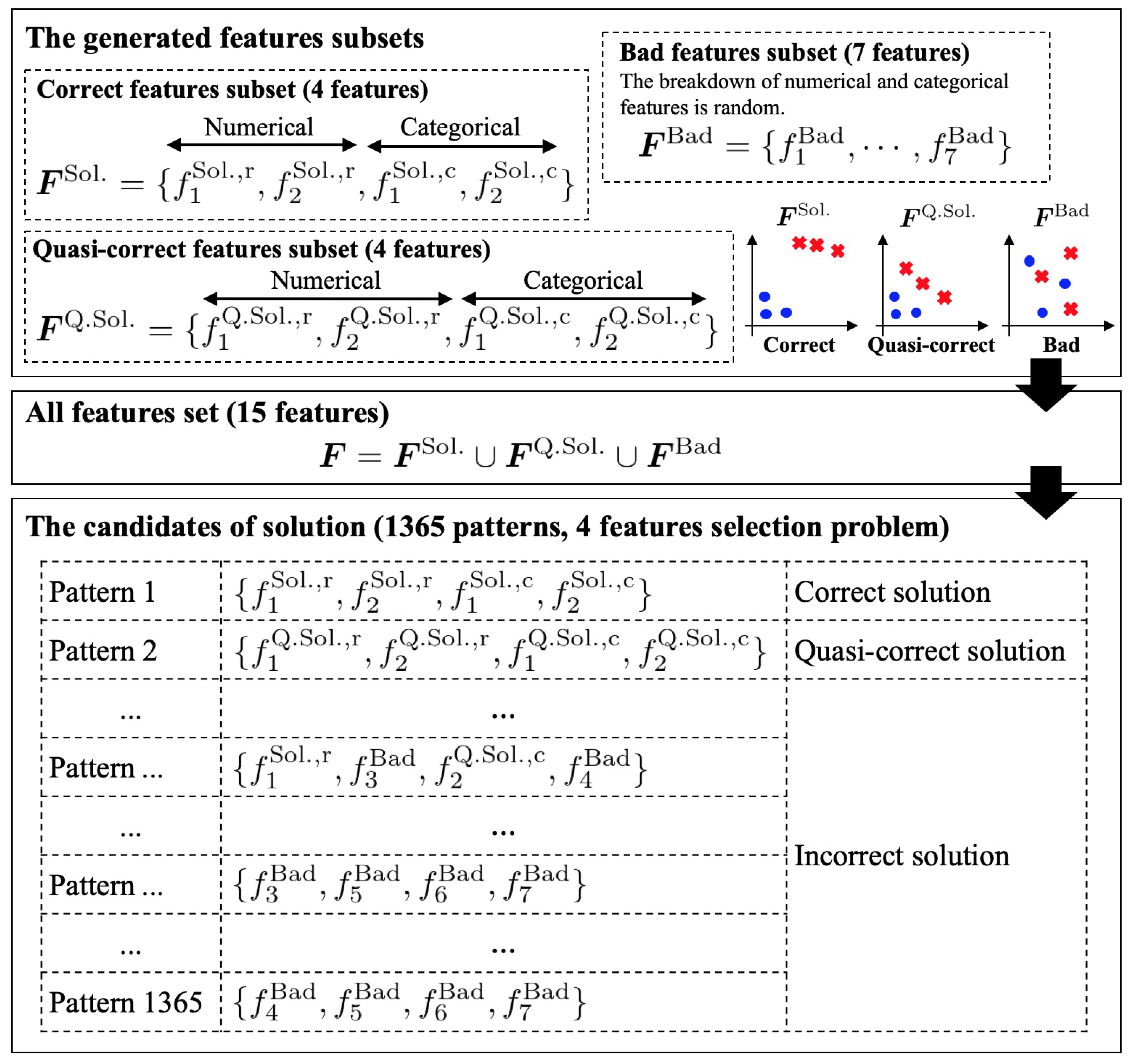
In this section, we describe whether the combination of the E2H MRS (Algorithm 1) and BS-FS (Algorithm 2) can determine an effective feature subset for classification. To this end, the following features are generated:

$$\begin{array}{c}\hfill \begin{array}{cc}\hfill & {\mathit{F}}^{\mathrm{Sol}.},\left|{\mathit{F}}^{\mathrm{Sol}.}\right|=4:\mathrm{Correct}\mathrm{feature}\mathrm{subset}\mathrm{by}(e^{\mathrm{c}},e^{\mathrm{r}})=(40,50),\hfill \\ \hfill & {\mathit{F}}^{\mathrm{Q}.\mathrm{Sol}.},\left|{\mathit{F}}^{\mathrm{Q}.\mathrm{Sol}.}\right|=4:\mathrm{Quasi}-\mathrm{correct}\mathrm{feature}\mathrm{subset}\mathrm{by}(e^{\mathrm{c}},e^{\mathrm{r}})=(40/2,50/2),\hfill \\ \hfill & {\mathit{F}}^{\mathrm{Bad}},\left|{\mathit{F}}^{\mathrm{Bad}}\right|=7:\mathrm{Bad}\mathrm{feature}\mathrm{subset},\hfill \\ \hfill & \mathit{F}={\mathit{F}}^{\mathrm{Sol}.}\cup {\mathit{F}}^{\mathrm{Q}.\mathrm{Sol}.}\cup {\mathit{F}}^{\mathrm{Bad}},\left|\mathit{F}\right|=15:\mathrm{All}\mathrm{features}\mathrm{set}.\hfill \end{array}\end{array}$$

(29)

Among these, ${\mathit{F}}^{\mathrm{Sol}.}$ is the most effective feature subset comprising two numerical and two categorical features (a total of four features), which are generated based on the probability distribution of $(e^{\mathrm{c}},e^{\mathrm{r}})=(40,50)$. Further, ${\mathit{F}}^{\mathrm{Q}.\mathrm{Sol}.}$ is a quasi-correct feature subset consisting of two numerical and two categorical features (a total of four features), and these features are generated based on the distribution of $(e^{\mathrm{c}},e^{\mathrm{r}})=(40/2,50/2)$. Next, ${\mathit{F}}^{\mathrm{Bad}}$ consists of seven randomly generated features (the breakdown of categorical and numerical features is also random). Therefore, ${\mathit{F}}^{\mathrm{Bad}}$ is not an effective classification feature subset. Notably, the feature sets $\mathit{F}$ consist of the union of these feature subsets, and the total number of features is $4+4+7=15$. We adopt the proposed algorithms E2H MRS and BS-FS to identify four effective features among all the 15 features. Note that the total number of solutions is ${}_{15}{\mathrm{C}}_4=1365$, as shown in Figure 5; that is, the chance of obtaining the optimal solution in one trial is $1/{}_{15}{\mathrm{C}}_4=1/1365\simeq 0.0733\%$.

Although both ${\mathit{F}}^{\mathrm{Sol}.}$ and ${\mathit{F}}^{\mathrm{Q}.\mathrm{Sol}.}$ are effective feature subsets for correct classification, ${\mathit{F}}^{\mathrm{Sol}.}$ is better than ${\mathit{F}}^{\mathrm{Q}.\mathrm{Sol}.}$ owing to the adopted parameters, $e^{\mathrm{c}},e^{\mathrm{r}}$. That is, ${\mathit{F}}^{\mathrm{Sol}.}$ is the best solution, and ${\mathit{F}}^{\mathrm{Q}.\mathrm{Sol}.}$ is the second-best solution. In any case, identifying these subsets is a difficult problem because there is only one in all 1365 feature subsets, as shown in Figure 5. When the number of generated samples is extremely small, the evaluation value of the best subset ${\mathit{F}}^{\mathrm{Sol}.}$ may not be the minimum value owing to randomness. In this case, the proposed algorithms may identify the best ${\mathit{F}}^{\mathrm{Sol}.}$ or the second-best ${\mathit{F}}^{\mathrm{Q}.\mathrm{Sol}.}$ subset depending on the number of samples generated. Therefore, we tested various sample sizes $(n_{{\mathrm{z}}_0},n_{{\mathrm{z}}_1})$ defined by Equation (28). Moreover, we adopted $b\in \{0,100\},\gamma \in \{0.1,1,10\}$ to understand the effects of the Bayesian optimization and Hamming weight on the evaluation results. The corresponding experiment was conducted using 100 random seeds to verify the correct detection rate of ${\mathit{F}}^{\mathrm{Sol}.}$ and ${\mathit{F}}^{\mathrm{Q}.\mathrm{Sol}.}$.

5.2. Result and Discussion

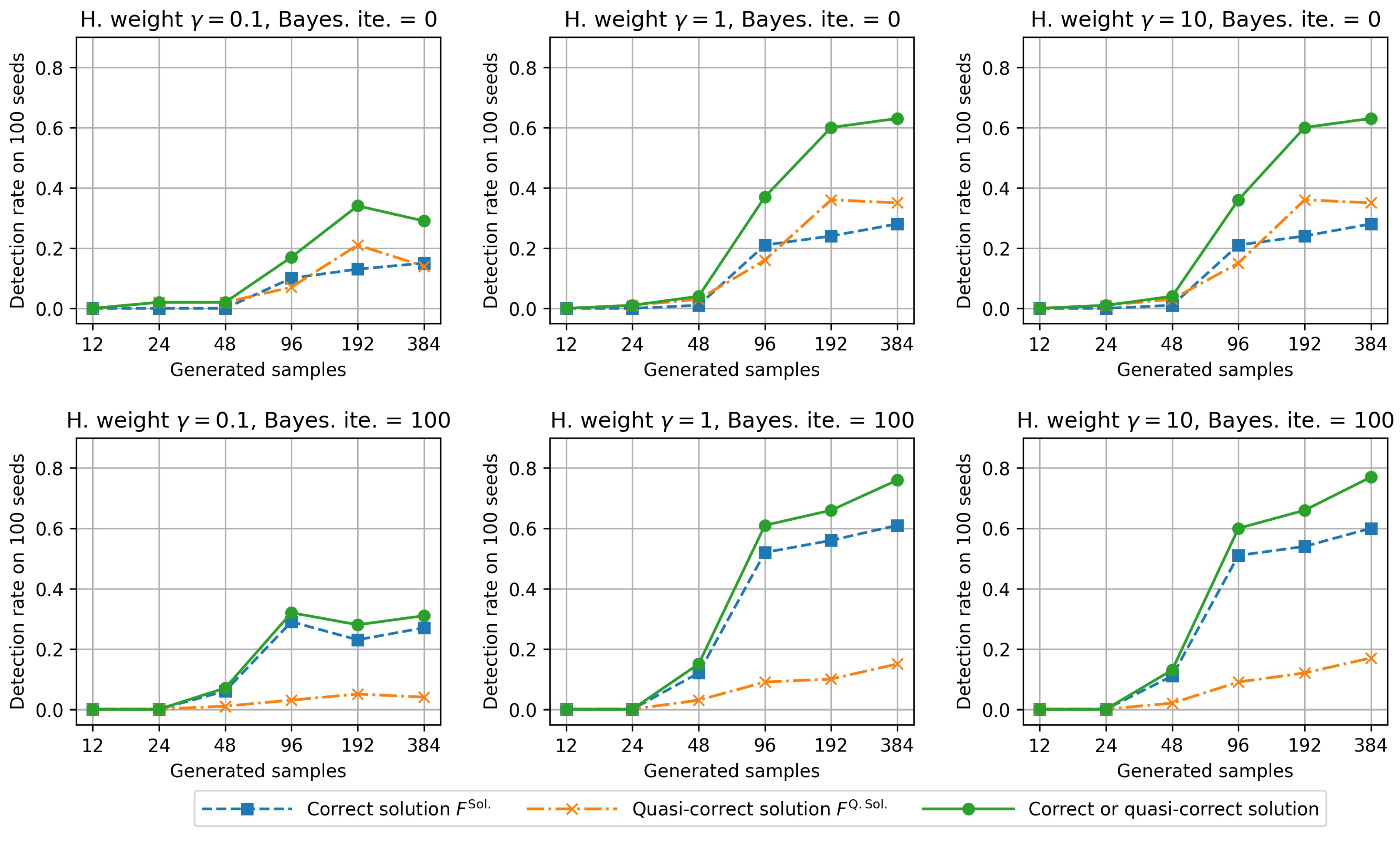
The rates for the correct detection of ${\mathit{F}}^{\mathrm{Sol}.}$ and ${\mathit{F}}^{\mathrm{Q}.\mathrm{Sol}.}$ for a total of 1365 solutions using the proposed algorithms are shown in Figure 6. The left-, center-, and right-side figures present the results for different Hamming weights. The top and bottom figures illustrate the results of the Bayesian optimization. The horizontal axis represents the number of generated samples, and the vertical axis represents the correct detection rate for 100 seeds.

First, when the Hamming weight is too small ($\gamma =0.1$), the correct detection rate is also small compared with that for $\gamma =1$ and $\gamma =10$. The Hamming weight refers to the weight of categorical features (see Equation (7)). Therefore, for $\gamma =0.1$, we consider that the detection rates decrease because the proposed method fails to detect correct categorical features. From the results for $\gamma =1$ and $\gamma =10$, we can conclude that the correct detection rates improve for a large Hamming weight. However, because the results for $\gamma =1$ and $\gamma =10$ are almost the same, there may be an upper limit to its effectiveness.

Next, we discuss the effects of Bayesian optimization. When Bayesian optimization was not adopted (upper side in Figure 6), the detection rates of ${\mathit{F}}^{\mathrm{Sol}.}$ and ${\mathit{F}}^{\mathrm{Q}.\mathrm{Sol}.}$ were almost the same. In contrast, when searching for the initial feature subset using Bayesian optimization (bottom side in Figure 6), the detection rate of ${\mathit{F}}^{\mathrm{Sol}.}$ was higher than that of ${\mathit{F}}^{\mathrm{Q}.\mathrm{Sol}.}$ by approximately three times. For example, when the number of generated samples was 384, the detection rates of ${\mathit{F}}^{\mathrm{Sol}.}$ and ${\mathit{F}}^{\mathrm{Q}.\mathrm{Sol}.}$ were approximately 60% and 20%, respectively. Therefore, searching the initial feature subset using Bayesian optimization may be effective in identifying the best subset ${\mathit{F}}^{\mathrm{Sol}.}$. Moreover, BS-FS is effective in detecting one of the following subsets: ${\mathit{F}}^{\mathrm{Sol}.}$ and ${\mathit{F}}^{\mathrm{Q}.\mathrm{Sol}.}$ because the total detection rate of ${\mathit{F}}^{\mathrm{Sol}.}$ and ${\mathit{F}}^{\mathrm{Q}.\mathrm{Sol}.}$ increases.

However, for small sample sizes, the detection rate of ${\mathit{F}}^{\mathrm{Sol}.}$ and ${\mathit{F}}^{\mathrm{Q}.\mathrm{Sol}.}$ is also small. When the sample size is too small, owing to an incorrect random bias, the E2H MRS may classify some features belonging to the bad feature subset ${\mathit{F}}^{\mathrm{Bad}}$ as effective. Therefore, when the sample size is too small, selecting only two patterns of the correct solution ${\mathit{F}}^{\mathrm{Sol}.}$ and quasi-correct solution ${\mathit{F}}^{\mathrm{Q}.\mathrm{Sol}.}$ from a total of 1365 pattern candidates is difficult when using E2H MRS and BS-FS. In actual data, cases where the numbers of collected samples are not large are sometimes encountered. In such cases, the selection of all the correct features becomes unrealistic. Therefore, it is important to check the number of correct features among the four features selected by the proposed method.

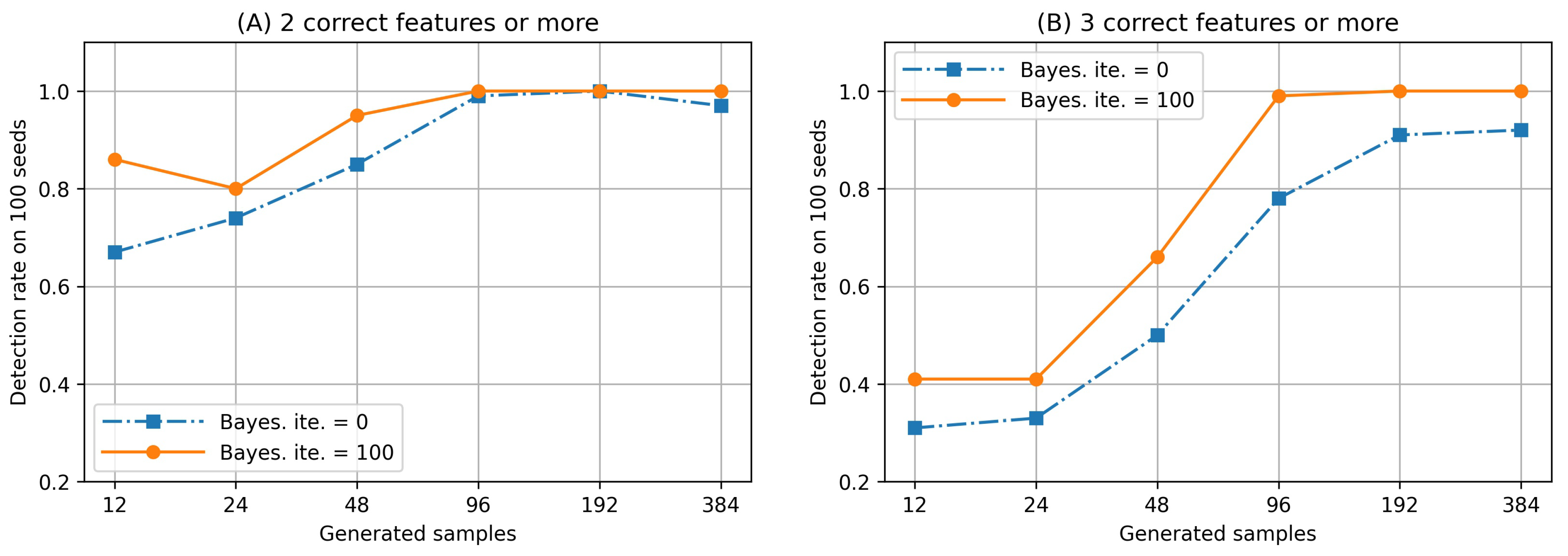
Further, we checked the detection rate of two or three correct features among the four features selected by the E2H MRS and BS-FS. Notably, the correct features are defined as features belonging to ${\mathit{F}}^{\mathrm{Sol}.}$ or ${\mathit{F}}^{\mathrm{Q}.\mathrm{Sol}.}$. The corresponding results are presented in Figure 7. Here, (A) and (B) denote the detection rates obtained when the number of correct features is two and three or more, respectively. As can be observed, although the sample size is small, some correct features are selected. Moreover, we also understand that the detection rates increase when searching for the initial feature subset using Bayesian optimization. Therefore, we consider that the proposed methods, E2H MRA and BS-FS, are effective in identifying desirable feature subsets for classification tasks, even if the sample size is small.

6. Conclusions

In this paper, we propose an improved form of the original MRS [18], which is a feature subset evaluation and selection algorithm. The improved algorithm is referred to as the E2H MRS. In particular, the E2H MRS (Algorithm 1) can evaluate numerical and categorical mixture feature subsets and consider the distance between different classes. Moreover, a subset selection algorithm for time complexity $\mathcal{O}(b+n)$, referred to as BS-FS (Algorithm 2), is proposed. The proposed methods are validated using Experiments 1 and 2 based on artificial data.

In this study, we verified the effectiveness of the proposed methods, E2H MRS and BS-FS, by using samples sizes of several tens to hundreds. However, recently, large datasets with several million samples have emerged, and we did not verify the effectiveness on such a dataset. Moreover, we adopted 2:2 as the proportion of numerical/categorical features in the experiment described in Section 5. Cases of other proportions should also be verified. Therefore, we plan to perform experiments in future.

References

1. Chandrashekar, G.; Sahin, F. A survey on feature selection methods. Comput. Electr. Eng. 2014, 40, 16–28. [Google Scholar] [CrossRef]
2. Gopika, N.; Kowshalaya, M. Correlation Based Feature Selection Algorithm for Machine Learning. In Proceedings of the 3rd International Conference on Communication and Electronics Systems, Coimbatore, Tamil Nadu, India, 15–16 October 2018; Springer: Berlin/Heidelberg, Germany, 2018; pp. 692–695. [Google Scholar]
3. Yao, R.; Li, J.; Hui, M.; Bai, L.; Wu, Q. Feature Selection Based on Random Forest for Partial Discharges Characteristic Set. IEEE Access 2020, 8, 159151–159161. [Google Scholar] [CrossRef]
4. Yun, C.; Yang, J. Experimental comparison of feature subset selection methods. In Proceedings of the Seventh IEEE International Conference on Data Mining Workshops (ICDMW 2007), Omaha, NE, USA, 28–31 October 2007; pp. 367–372. [Google Scholar]
5. Lin, W.C. Experimental Study of Information Measure and Inter-Intra Class Distance Ratios on Feature Selection and Orderings. IEEE Trans. Syst. Man Cybern. 1973, 3, 172–181. [Google Scholar] [CrossRef]
6. Huang, C.L.; Wang, C.J. A GA-based feature selection and parameters optimizationfor support vector machines. Expert Syst. Appl. 2006, 31, 231–240. [Google Scholar] [CrossRef]
7. Stefano, C.D.; Fontanella, F.; Marrocco, C.; Freca, A.S.D. A GA-based feature selection approach with an application to handwritten character recognition. Pattern Recognit. Lett. 2014, 35, 130–141. [Google Scholar] [CrossRef]
8. Dahiya, S.; Handa, S.S.; Singh, N.P. A feature selection enabled hybrid-bagging algorithm for credit risk evaluation. Expert Syst. 2017, 34, e12217. [Google Scholar] [CrossRef]
9. Li, G.Z.; Meng, H.H.; Lu, W.C.; Yang, J.Y.; Yang, M.Q. Asymmetric bagging and feature selection for activities prediction of drug molecules. BMC Bioinform. 2008, 9, S7. [Google Scholar] [CrossRef] [Green Version]
10. Loh, W.Y. Fifty Years of Classification and Regression Trees. Int. Stat. Rev. 2014, 82, 329–348. [Google Scholar] [CrossRef] [Green Version]
11. Loh, W.Y. Classification and regression trees. Data Min. Knowl. Discov. 2011, 1, 14–23. [Google Scholar] [CrossRef]
12. Roth, V. The generalized LASSO. IEEE Trans. Neural Networks 2004, 15, 16–28. [Google Scholar] [CrossRef]
13. Osborne, M.R.; Presnell, B.; Turlach, B.A. On the LASSO and its Dual. J. Comput. Graph. Stat. 2000, 9, 319–337. [Google Scholar] [CrossRef]
14. Bach, F.R. Bolasso: Model Consistent Lasso Estimation through the Bootstrap. In Proceedings of the 25th International Conference on Machine Learning, Helsinki, Finland, 5–9 July 2008. [Google Scholar] [CrossRef]
15. Palma-Mendoza, R.J.; Rodriguez, D.; de Marcos, L. Distributed ReliefF-based feature selection in Spark. Knowl. Inf. Syst. 2018, 57, 1–20. [Google Scholar] [CrossRef] [Green Version]
16. Huang, Y.; McCullagh, P.J.; Black, N.D. An optimization of ReliefF for classification in large datasets. Data Knowl. Eng. 2009, 68, 1348–1356. [Google Scholar] [CrossRef]
17. Too, J.; Abdullah, A.R. Binary atom search optimisation approaches for feature selection. Connect. Sci. 2020, 32, 406–430. [Google Scholar] [CrossRef]
18. Chen, X.W.; Jeong, J.C. Minimum reference set based feature selection for small sample classifications. ACM Int. Conf. Proc. Ser. 2007, 227, 153–160. [Google Scholar] [CrossRef]
19. Mori, M.; Omae, Y.; Akiduki, T.; Takahashi, H. Consideration of Human Motion’s Individual Differences-Based Feature Space Evaluation Function for Anomaly Detection. Int. J. Innov. Comput. Inf. Control. 2019, 15, 783–791. [Google Scholar] [CrossRef]
20. Zhao, Y.; He, L.; Xie, Q.; Li, G.; Liu, B.; Wang, J.; Zhang, X.; Zhang, X.; Luo, L.; Li, K.; et al. A Novel Classification Method for Syndrome Differentiation of Patients with AIDS. Evid.-Based Complement. Altern. Med. 2015, 2015, 936290. [Google Scholar] [CrossRef] [Green Version]
21. Mori, M.; Flores, R.G.; Suzuki, Y.; Nukazawa, K.; Hiraoka, T.; Nonaka, H. Prediction of Microcystis Occurrences and Analysis Using Machine Learning in High-Dimension, Low-Sample-Size and Imbalanced Water Quality Data. Harmful Algae 2022, 117, 102273. [Google Scholar] [CrossRef]
22. Zhao, Y.; Zhao, Y.; Zhu, Z.; Pan, J.S. MRS-MIL: Minimum reference set based multiple instance learning for automatic image annotation. In Proceedings of the International Conference on Image Processing, San Diego, CA, USA, 12–15 October 2008; pp. 2160–2163. [Google Scholar]
23. Cerda, P.; Varoquaux, G. Encoding High-Cardinality String Categorical Variables. IEEE Trans. Knowl. Data Eng. 2022, 34, 1164–1176. [Google Scholar] [CrossRef]
24. Beliakov, G.; Li, G. Improving the speed and stability of the k-nearest neighbors method. Pattern Recognit. Lett. 2012, 33, 1296–1301. [Google Scholar] [CrossRef]
25. Bentley, J.L. Multidimensional binary search trees used for associative searching. Commun. ACM 1975, 18, 509–517. [Google Scholar] [CrossRef]
26. Ram, P.; Sinha, K. Revisiting kd-tree for nearest neighbor search. In Proceedings of the ACM International Conference on Knowledge Discovery and Data Mining, Anchorage, AK, USA, 4–8 August 2019; pp. 1378–1388. [Google Scholar]
27. Ekinci, E.; Omurca, S.I.; Acun, N. A comparative study on machine learning techniques using Titanic dataset. In Proceedings of the 7th International Conference on Advanced Technologies, Hammamet, Tunisia, 26–28 December 2018; pp. 411–416. [Google Scholar]
28. Kakde, Y.; Agrawal, S. Predicting survival on Titanic by applying exploratory data analytics and machine learning techniques. Int. J. Comput. Appl. 2018, 179, 32–38. [Google Scholar] [CrossRef]
29. Huang, Z. Extensions to the k-Means Algorithm for Clustering Large Data Sets with Categorical Values. Data Min. Knowl. Discov. 1998, 2, 283–304. [Google Scholar] [CrossRef]
30. Wen, T.; Zhang, Z. Effective and extensible feature extraction method using genetic algorithm-based frequency-domain feature search for epileptic EEG multiclassification. Medicine 2017, 96. [Google Scholar] [CrossRef] [PubMed]
31. Song, J.; Zhu, A.; Tu, Y.; Wang, Y.; Arif, M.A.; Shen, H.; Shen, Z.; Zhang, X.; Cao, G. Human Body Mixed Motion Pattern Recognition Method Based on Multi-Source Feature Parameter Fusion. Sensors 2020, 20, 537. [Google Scholar] [CrossRef]
32. Bergstra, J.; Bardenet, R.; Bengio, Y.; Kégl, B. Algorithms for hyper-parameter optimization. Adv. Neural Inf. Process. Syst. 2011, 42. [Google Scholar]
33. Optuna: A Hyperparameter Optimization Framework. Available online: https://optuna.readthedocs.io/en/stable/ (accessed on 1 November 2022).
Figure 1. Issues related to the original minimum reference set (MRS) [18] feature selection algorithm.
Make 05 00007 g001
Figure 2. Overview of the probability distributions defined by Equations (21) and (23) for generating artificial data. The blue and red circles represent the distributions used for generating samples belonging to z 0 and z 1 , respectively. The number of blue circles on each figure is one because samples belonging to class z 0 are generated by the Gaussian distribution. The number of red circles is three because the samples of class z 1 are generated based on a Gaussian mixture distribution. The radius of the circle represents the standard deviation. These figures indicate that the average values of these distributions are changed by x 3 and x 4 , the values of categorical features. Therefore, to correctly classify classes z 0 and z 1 , categorical features should be used. We used artificial samples generated by these distributions for verifying the effectiveness of the proposed methods E2H MRS and BS-FS. These results are described in Section 4 and Section 5.
Make 05 00007 g002
Figure 3. Artificial data generated by using Equations (21) and (23), and Figure 2. The cases (A)–(D) vary in parameters e c and e r . The values of categorical features x 3 and x 4 change from left to right. The rightmost figure presents an explicit scatter plot of the numerical features x 1 , x 2 , i.e., no categorical features x 3 , x 4 are considered.
Make 05 00007 g003
Figure 4. Effect of the distance weight δ on the evaluation L ( F ) .
Make 05 00007 g004
Figure 5. The generated feature subsets for the experiment 2 and the candidates of solutions.
Make 05 00007 g005
Figure 6. Detection rate of F Sol . and F Q . Sol . for the E2H MRS and BS-FS (Bayesian optimization iteration b { 0 , 100 } , and Hamming weight γ { 0.1 , 1 , 10 } ).
Make 05 00007 g006
Figure 7. Detection rate of two or three correct features (Hamming weight γ = 1 and Bayesian iteration b { 0 , 100 } ).
Make 05 00007 g007