1. Introduction
It has been understood for a while that pruning a network after training can lead to much smaller networks that still maintains similar accuracy to the original network. However, the question arises, if these smaller networks perform just as well as the larger ones, could one not train the smaller network architecture to begin with?
The lottery ticket hypothesis states, “a randomly-initialized, dense neural network contains a subnetwork that is initialized such that—when trained in isolation—it can match the test accuracy of the original network after training for at most the same number of iterations” [
1]. These smaller networks are referred to as “winning tickets”. The process of finding winning tickets was proposed to start with an initial set of weights, train the network, prune the network, and finally reset the remaining weights back to their initial state.
It has been shown that these winning tickets perform as well, or sometimes better and require less time to train when compared to the original network. In this paper, we focus on applying this hypothesis to tabular neural networks (TNN) for several datasets to generate smaller networks with similar performance. This is not well tested among other research and most smaller datasets do not get optimized in research. This work not only tries to improve leading tabular model performance, but sets some clear leading benchmarks for several tabular datasets while making the model available for any tabular dataset for comparison that other researchers wish to test and compare [link to code omitted during review stage]. The code just requires the dataset loaded with categorical and continuous features labelled and usual parameter tuning such as learning rate.
We use tabular neural networks from FastAI [
2] which work on the principle of converting categorical features into embeddings. The models come with strong features such as normalization of continuous features, filling in missing data, and converting dates into categorical features. The models can be trained with their cycle training approach which raises and lowers the learning rate to find the best local minimum while training. We chose the model for its ability to process categorical features as embeddings while being a lightweight neural network to obtain remarkably small models during pruning while outperforming standard/go-to models for tabular data such as random forest and gradient boosting.
There are many small tabular datasets which often do not get optimized in research. These datasets are filled with categorical features and missing entries while often having few samples to test. In this paper, we use the lottery ticket hypothesis to improve FastAI’s tabular neural network to easily prune models for any tabular dataset. We test a wide range of datasets from large to small including different ranges of categorical and continuous features. In addition, we compare and evaluate several tabular models to the tabular neural network.
The lottery ticket hypothesis was first tested on dense neural networks and convolutional neural networks for MNIST and CIFAR10 [
1]. The authors achieved networks 80–90% smaller while both creating faster networks and increasing the accuracy of the models in comparison to the original sized models. The authors show that while pruning has been around for a long time, pruning networks often lead to more difficult training with less accuracy. By finding the lottery tickets of a network, difficulty in training of smaller networks is reduced while accuracy can be maintained and even exceed the original model.
Since its introduction, there have been many papers testing the lottery ticket hypothesis on different architectures. In this case authors look to find winning tickets in networks by searching for common winning tickets across many datasets [
3]. They test on a range of image datasets such as Fashion MNIST, SVHN, CIFAR-10/100, ImageNet, and Places365. Their findings were that winning tickets generalized over many datasets, but interestingly the larger datasets produced better winning tickets that were more generalizable than those from smaller datasets. When testing the lottery ticket hypotheses for object detection [
4] authors achieving a sparsity of up to 80%.
There have been tests on the lottery ticket hypothesis on increasingly larger graph neural networks (GNN) [
5]. For node classification tasks, they show a decrease in multiply-accumulate operations (MACs) of up to 98% while having a sparsity of nearly 98% with minimal affect to performance. For linking predictions, they show similar sparsity with a large reduction in MACs.
The field of natural language processing (NLP) has recently exploded with new models since the introduction of the transformer architecture [
6]. The models grow increasingly large, from sizes like the popular BERT [
7] architecture of up to 350 million parameters to sizes like GPT-3 [
8] reaching up to 175 billion parameters. Ref. [
9] prune the BERT architecture, but they begin from the pretrained state and test the lottery ticket hypothesis using downstream tasks. The paper only applies unstructured pruning stating “since we perform a scientific study of the lottery ticket hypothesis rather than an applied effort to gain speedups on a specific platform, we use general-purpose unstructured pruning” [
9]. With unstructured pruning, they are able to find networks with sparsity of 40–90% while testing a range of downstream tasks.
Tabular models are heading towards larger networks as well with the recent transformer architecture making its way to tabular data. Authors proposed a time series BERT architecture for tabular data called TabBERT [
10] and a tabular data generator TabGPT based on the GPT architecture. In one case [
11] authors use transformers to convert text in tabular data into features and released a package to process the data. TabTransformer [
12] uses the transformer architecture to achieve new SOTAs and tested on 15 datasets, competing well with ensemble approaches.
In this paper, we focus on tabular dense neural networks with the goal to prune them as much as possible while maintaining accuracy utilizing the lottery ticket hypothesis. We test our models on 8 datasets of different varieties and show competing results for datasets with available comparisons.
2. Materials and Methods
In this section, we first describe the datasets evaluated and their various features. Then we describe the pruning methods evaluated including our new pruning approach on iterative.
2.1. Datasets
In this section, we describe the tabular datasets used in our experiments. The goal in dataset selection is to test many varieties of tabular data. Some datasets are of poor quality using poor features and duplicate/missing data, or small in size with a few hundred samples. Other datasets are large with good quality data, while some use simulated data augmentation to generate millions of samples. Some datasets have a predefined test set, others do not have a defined prediction goal. Each dataset has a variety of tabular features, some containing just continuous features, others containing only categorical features, and many mixed with both. The datasets are described in more detail in this section, and we present the number of samples, number of features, evaluation metrics, and train-validation-test splits used in our experiments in
Table 1.
The first dataset is the Alcohol dataset [
13]. It is our smallest dataset and contains the most diverse mix of continuous and categorical features. The dataset contains information on students such as school, gender, age, information like hobbies and goals, their family and related information such as work, education, size, etc. As quoted from this recent dataset survey [
14], “This dataset has also been uploaded on Kaggle where 305 publicly available kernels perform exploratory data analysis. Unfortunately, there is not defined any task with specific validation metric such that there is no leaderboard publicly available”, so we used the workday alcohol consumption of the student as the final goal. The model aims to predict the students’ workday alcohol consumption which is a target range of 1 to 5 where 1 is very low and 5 is very high consumption.
The next dataset is the Video Games Sales dataset (
https://github.com/GregorUT/vgchartzScrape,
https://www.kaggle.com/gregorut/videogamesales, accessed on 26 September 2022). The dataset also does not have a clear final goal or leaderboard information. There are features of videos games such as rank, publisher, year and Genre and sales information. We have information on sales for North America, Europe, Japan, other countries and global sales. Predicting global sales means we would have to omit information about sales in other countries as it would be just a simple sum of those sales, so we decided to predict North American sales given information on the video game and sales information in other countries not including global sales.
The Wine Quality dataset [
15] aims to predict a quality score between 0 and 10 of the wine given its features. The features are continuous values representing different acidity rates, sugar levels, density, pH and more.
The Chocolate Ratings dataset (
https://www.kaggle.com/rtatman/chocolate-bar-ratings, accessed on 26 September 2022) was created to generate expert opinions on chocolate. We must predict the expert ratings which are values between 1 and 5 where 1 is bad taste and 5 is the best taste. The features include the company, location, type of beans, percentage of cocoa, and origin information.
The Poker Hand dataset [
16] is an extremely large selection of poker hands. Each sample is a set of 5 cards indicating the card numbers as 5 features and their suits as 5 more features. The final goal of this dataset is to predict the poker hand such as 0 for nothing, 1 for one pair, 2 for two pairs, 3 for three of a kind, 4 for a straight, 5 for a flush, 6 for a full house, 7 for four of a kind, 8 for straight flush, and 9 for a royal flush. We used this as a regression problem where higher (9) the better hand and lower (0) the worse the hand.
The Titanic dataset (
https://www.kaggle.com/c/titanic/data, accessed on 26 September 2022) uses information on passengers of the Titanic to predict whether they survived. The features include gender, cabin, location of embarkment, ticket class (1st, 2nd, 3rd), number of siblings or spouses, number of parents or children, age and fare. The goal is to predict the survival of the individual (yes or no) using F1 as a metric. There is a predefined test set without labels which must be submitted through Kaggle to be evaluated, but our results reflect a train/validation/test split from the labelled train set only. We also take our best available model for this dataset and run it through Kaggle to get a test score for their test set in the experiments section. Note that a new dataset Titanic Extended (
https://www.kaggle.com/pavlofesenko/titanic-extended, accessed on 26 September 2022) was introduced with many more features while minimizing the number of empty features derived from the literature allowing others to achieve 100% accuracy, so we opted to use the more difficult prior version for testing without knowledge of the extended features and containing missing information.
The Health Insurance dataset (
https://www.kaggle.com/anmolkumar/health-insurance-cross-sell-prediction, accessed on 26 September 2022) aims to predict vehicle insurance sales to customers of health insurance. We are given information on the policy holder such as a unique ID (omitted in training), gender, age, has a driving license, region, types of vehicle information like age and damage, and information on their premiums. The goal is whether the customer will accept the vehicle insurance which is a binary prediction using F1 as a metric.
The Susy dataset [
17] is our largest dataset containing 4 million training samples, 500k validation and 500k test samples. The test set was predefined for this dataset as the last 500k samples in the list. The dataset contains simulation data of a particle collider with the goal to find rare particles. There are eight kinematic features of the collision and 10 functions of those features with the final goal distinguishing signal from background using F1 as a metric.
2.2. Methodology
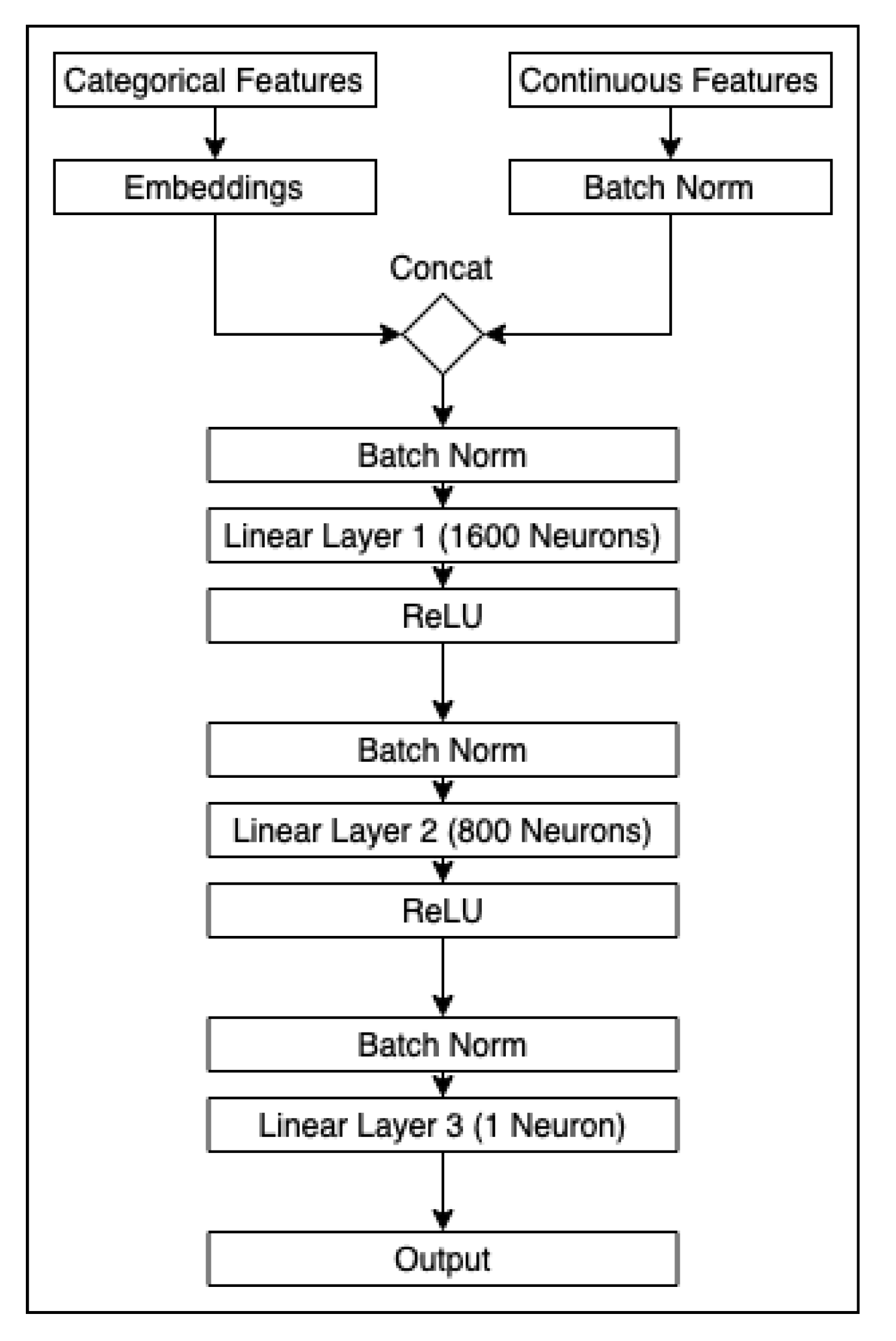
To predict on these datasets, we use tabular neural networks repurposed from FastAI [
2] with cycle training procedures. FastAI’s tabular model architecture is shown in
Figure 1. It starts with a concatenation of categorical embeddings and continuous features, then linear layers follow with optional batch normalization at each stage. We implemented batch normalization in the pruning process as an optional parameter, but results were better without the batch norm layers and removing them left us with smaller and faster models (also removed for the original model for fair speed comparisons). The cycle training procedure increases and reduces the learning rate as needed to reach the best local minimum, so we are able to set standard learning rates for all models of a dataset and automatically train our pruning approaches. The FastAI tabular structure is well suited to obtain leading results and we improve the model in terms of accuracy and speed through cycles of pruning in this paper. We kept the number of training epochs the same for all pruned versions of a dataset as defined by the lottery ticket hypothesis and used early stopping to avoid overfitting the models based on validation scores. The data was preprocessed by converting categorical features to embeddings, filling missing values and normalizing continuous features.
The models were altered to allow pruning of full nodes selected by different pruning selection strategies to improve inference time. Pytorch provides functionality to select weights to prune with L1 norm pruning, a generic LN norm pruning, and random pruning. We chose the popular default methods provided by Pytorch L1 and random and including the case where we do not select a norm such as N = −inf. N = 1 selects nodes based on the sum of all weights thus pruning nodes with large weights. So, the reasoning for N = −inf was to select nodes based on the smallest weight. The approach we describe ideally finds optimal nodes based on a few tests of N = 1 (largest), N = −inf (smallest) or something between using random pruning. We pruned all weights associated with nodes from the linear layers of the model depending on a rate P where the Pytorch functions provide a mask on the nodes setting all the weights to 0.
While the pruning functionality provided by Pytorch is useful for testing, we wanted the full benefit of smaller models which provide inference and training time improvements rather than a mask over the weights which still require computation. In this case we designed a simple approach to fully prune the weights. First, we save the initial untrained weights of the model W0. Then we train the model until we reach the optimal validation stopping point and record the weights W1. Next, we generate pruning masks for W1 depending on the selected norm (or random) and pruning rate P, then apply the masks on the initial untrained weights W0. The remaining subset of weights from W0 will be copied over to a smaller blank model sized appropriately for the non-zero weights. Finally, we continue to train the pruned model depending on the iterative or one-shot styles described below using the smaller network.
2.2.1. Iterative Pruning
A simple iterative approach can be thought of as starting with a model size and reducing it slowly until we reach an optimal size based on criteria for accuracy and speed performance. The iterative approach uses a pruning rate p = 0.5 (50%) which we found to be suitable for scaling the model down without leaping over quality model reductions. First, we describe the standard iterative approach in our tests using a large model potentially containing many lottery tickets. Second, we describe an alteration to the iterative approach by first selecting a well performing model not necessarily large in size, then pruning this model which ideally contains higher quality lottery tickets (perhaps not as many to find).
The first approach uses a starting point of a large model [1600, 800] where the parameters are the sizes of the linear layers, respectively. We call this starting point the original model. We train the original model, prune it at the rate of P, then repeat on the pruned model until we reach the smallest state possible (ideally [1, 1]). We evaluate each size to find an optimal reduction point for each dataset.
More formally, for a given model with weights and nodes [, ], we apply a prune rate of P onto the nodes iteratively for all states k with nodes [, ] and weights where is a subset of and for all k. The pruned nodes at each state k are selected by training the weights of and selecting them based on a given measure of norm, then is the the set of remaining weights reset to their original starting point in . The validation score of each state of trained weights are recorded and used to select the optimal prune state k.
In the second approach, we instead train at various starting points of different model sizes starting with [1600, 800], then continuing with [800, 400] and so on reducing the size by 50% at each step. We train each original model in search of the best starting point for the best performing model. In other words we search for the best in terms of model size [, ] (selected based on validation score) and start our pruning strategy at using the first iterative strategy to find an optimal state k where . We run iterative pruning like described in the first approach on this potentially smaller model ideally containing better lottery ticket weights available for the pruning strategy to select (instead of a large selection and stopping at a local minima of lower quality weights).
The second approach naturally searches for the optimal model size from the start which already increases accuracy of the model compared to other tabular approaches compared in the results section, then adding pruning finds even smaller sizes while potentially increasing accuracy. Thus, the clear difference between our suggested second approach and the standard first approach is model size. Both can maintain accuracy in a similar manner, but the second approach is able to do so with a smaller model size in general.
2.2.2. One-Shot Pruning
The one-shot pruning approach works like iterative, but uses a prune rate of P = 1.0. This means we prune the entire model with weights in one shot reducing it down entirely to a size of [, ] and weights . We adapted one-shot pruning to run on all the potential starting points we described in iterative (second approach), then we select the best performing one-shot model. We find in general one-shot does not perform well, but is included in our results for comparisons. This result highlights the benefit of finding an optimal stopping point using iterative without pruning weights too hastily.
3. Experimentations, Results, and Discussion
The goal of our paper is to set a new standard comparison for all tabular datasets using the best pruning strategy for tabular models while optimizing inference speeds. Thus, we present results on three important factors to this goal. The first demonstrates our ability to reduce train and inference times, the second presents a set of results for our best performing models on a wide variety of datasets, and the last is a comparison to a variety of other tabular approaches to show a clear lead in results. We also run an optimization for model size with minimal affect to accuracy.
In all tests, all random seeds were set to the same value to allow fair comparisons and reproducibility of any result shown. We paid careful attention to have the model weights set to the same initial states for all styles of pruning and datasets fixed and batched exactly the same, thus the only change is in model size and weight select which are exact subsets of the original model. Training has early stopping after a fixed number of epochs for each dataset. The computations were made on a 2-CPU system for all tests, no use of a GPU. It is important for us to show that these models can run fast on a CPU machine which is ideal for any kind of application especially with low-hardware requirements, or give any researcher the ability to use these models.
3.1. Train and Inference Time per Model Size
Table 2 and
Table 3 show the time taken to run the tabular models. The first table contains the training times averaged over all epochs while the second contains the inference time on the test set. The tables present the number of seconds taken and the reduction of time in percentage compared to the largest model. The trend shows that a smaller model can lead to faster training and faster inference until we reach extremely small models of a few nodes, at which point improvement time between small models is down to a few milliseconds difference which can be masked by possible noise on the processor running other tasks. The small datasets of a few hundred samples do not provide much insight, but the larger datasets show a better downtrend. These results show us that it is not necessary to prune down to the smallest state possible for speed improvements while we attempt to find an optimal size for accuracy.
3.2. Dataset Accuracy
Table 4 highlights our best performing models accuracy-wise. In bold are the models with the best accuracy. The table presents the RMSE or F1 depending on the dataset task, the size of the model, the difference in percentage compared to the original model, and the pruning mode that generated the result. Iterative on the largest model (approach 1) has the best likelihood of generating a better model with 5/8 datasets improving. Iterative on the best performing model (approach 2) has one best case tied with approach 1 for the poker dataset, but it happens that the largest model was the best performing model, so both approaches generated the same result. Meanwhile approach 2 can maintain similar accuracy in many datasets while lowering the model size by a substantial margin (all datasets show less than or equal model sizes compared to approach 1). For example, the chocolate dataset maintains exactly the same accuracy loss between both approaches, but we were able to find the smallest possible model state [1, 1] compared to the large [200, 100] of approach 1. Other notable examples are the health ([200, 100] to [7, 3]) and Susy ([200, 100] to [100, 50]) datasets which are our largest test sets. One-shot had one case of generating a best performing model for the smallest dataset in our experiments. There were two datasets, Wine and Chocolate, which could not be pruned further without some loss in accuracy, but they can be pruned extremely small with little degradation in accuracy.
3.3. Comparison to Tabular Models and Other Approaches
We compare the tabular models to other models in
Table 5 and found that even the original model has the best performing accuracy for all but a few results. In this case the Health dataset using SVM/RF and Susy using GB resulted in a better accuracy than the original model, all comparisons shown are to the original tabular model. The table shows the following models: K Nearest Neighbors (KNN), Linear Regression (LR), Support Vector Machine (SVM), Gradient Boosting (GB), Decision Tree (DT) and Random Forest (RF). We also used the equivalent classifier version of these models for the classification tasks using F1 as a measure of accuracy. All models were tested on the exact same train, validation and test sets and we also preprocessed the data in the same way converting text/categorical features to values, normalizing continuous features and filling in missing values. All models were tuned appropriately for each dataset individually, the best parameters were selected based on their validation score and present the test score in the table. Note that Susy has KNN and SVM missing, this is because even with a 32 CPU machine and weeks of computation we could not produce a result in a reasonable timeframe, so we omitted them from the table. To fully train these models several times over for parameter tuning on a large dataset like Susy would be costly and time consuming, if it is computationally feasible. This highlights the benefit of having a faster model such as our pruned tabular neural network that can scale appropriately for large datasets with minimal resources such as CPUs (using 2 or less).
In comparison with other approaches, some datasets do not have reported results such as Video Games, Alcohol and Chocolate. The Titanic dataset is shown on Kaggle to achieve 100% on the test set using random forest and other approaches due to an extended features dataset derived from the literature. We used the version without extended features, thus running our best model (L1 iterative [13, 7]) on Kaggle’s test set gives us a score of 0.77511, but the result is incomparable to those using the extended features achieving perfect results. Because of missing available comparisons, we provide comparisons using exactly the same data split and preprocessing for all datasets using several models in
Table 5 as mentioned previously.
For the Red Wine dataset, this paper [
18] reports the following RMSE results: 0.63245 using a 3 layer neural network, 0.61163 using GB, 0.62145 using SVM, and 0.62201 using ridge regression. In this case we hold the best result with 0.59206 RMSE (+3.200%) using an original tabular model sized at [100, 50].
This paper [
19] reports several F1 scores on the Health dataset: 0.80 using KNN, 0.77 using naïve bayes, 0.76 using LR, 0.81 using RF, 0.80 using MLP, 0.72 using SVM. Our best model using random iterative pruning (approach 1) and a size of [200, 100] achieves an F1 score of 0.82428 (+1.763%).
This paper [
20] reports accuracy as their metric and achieve the following results on the Poker dataset: 0.7687 using the Heterogeneous Dynamic Ensemble Selection based on Accuracy and Diversity (HDES-AD) approach, and 0.9068 using their HDES-ADP variant. They also report a comparison to Diversity for Dealing with Drifts (DDD) [
21] with 0.7867, Online Accuracy Updated Ensemble (OAUE) [
22] with 0.7325, and Active Fuzzy Weighting Ensemble (AFWE) [
23] with 0.7126. These approaches all use techniques to train ensembles of models and in particular [
20] generates models based on diversity and accuracy. We used RMSE instead of accuracy, but reran our models using F1 to optimize the models for this comparison. We achieved 0.87915 F1, 0.88360 accuracy (−2.558%) using L1 iterative [800, 400] (approach 1), and a similar score with a smaller model 0.87958 F1, 0.88462 accuracy (−2.446%) using Random iterative [400, 200] (approach 1).
Authors in this paper [
24] use a 70/30 train-test split on the Susy dataset at random. We used the recommended test set provided for our results of 10% in size using the final 500k samples in the list and a validation set of 10%. They report accuracy as their metric with the following scores: 0.7884 using LR, 0.774 using RF, 0.7546 using DT, 0.793 using GB. We achieved a better result of 0.77109 F1 using L1 iterative [200, 100] (approach 1), and an accuracy of 0.80285 (+1.242%).
3.4. Optimizing for Model Size Only
Finally, as our last result, we show a comparison of model size to the original tabular model by selecting the smallest model we can with less than 2% divergence in RMSE or F1. The goal of this test is to find the smallest model possible allowing for a small margin of error. We do the same with the original models, so we select the best size for original with less than 2% divergence in accuracy from the best performing RMSE/F1 original model. Then we apply the same rule to iterative and finally one-shot. The results are shown in
Table 6 highlighting in bold the smallest model following the described conditions. We show the original model size, then we present the difference in accuracy of other models and the prune rate from the same original model. In 7 out of 8 datasets we can generate a smaller model with minimal affect to RMSE/F1 including original with selection. In 6 of 8 datasets we outperform original with selection for 2% divergence generating models over 85% smaller and many over 98% smaller.
4. Conclusions and Future Work
In conclusion, we presented two approaches to pruning tabular neural networks, iterative and one-shot, based on the lottery ticket hypothesis using structured node pruning. We presented our variation of the iterative approach (2) which highlights its ability to find smaller models with similar performance in accuracy to the original iterative approach (1). The results are presented for 8 tabular datasets of different sizes and feature sets. We improved accuracy in 6 of the 8 datasets when considering accuracy alone. We also show up to 85% reduction in nodes in 6 of 8 datasets considering model size with limited affect to RMSE/F1 and over 98% reduction for many of them. We show that the tabular models outperform several other tabular models where comparisons were not available such as KNN, RF, SVM, DT, LR and GB. Finally, when comparing to other papers, we show an improvement of +3.200% in RMSE for the Wine dataset, +1.763% in F1 for the Health dataset and +1.242% in accuracy for the largest dataset of 5 million samples, Susy.
We found that the iterative approach while pruning a large model obtains the majority of top results compared to pruning better but smaller models, or in comparison to one-shot pruning. We go beyond just masking weights and implement a structured pruning approach reducing the model architecture to layer sizes as low as [1, 1] while improving accuracy in comparison to large model sizes like [1600, 800] for the alcohol dataset. Finally, for each dataset, we show the advantage in training and inference time of structured pruning at each pruning state. Future work will be focused on pruning layers once the size of a layer reaches one node, and other focuses will be on feature selection using the lottery ticket hypothesis where pruning nodes responsible for certain features will result in the removal of that feature.
While this approach shows improvements in terms of model size, training time, inference time, and in many cases accuracy, there are some limitations. The approach currently requires the original model to be trained in order to select lottery tickets, then retrained to evaluate the smaller model. In addition to this limitation, the selection process of the weights are limited to the method used to measure the weights. While they show improvements, they do not allow us to directly choose the model size and depend on us finding an optimal state. Future work would focus on removing any need to train the original model while allowing us to focus on weight selection for a given size rather than weight reduction to an arbitrary size.
We asked the question “if these smaller networks perform just as well as the larger ones, could one not train the smaller network architecture to begin with?”, and we believe it is clear that given the right set of initial weights for the network, a smaller, faster and better network can be trained to begin with. We show the existence of these weights through iterations of pruning, so perhaps there exists an approach to initializing the network as a function of the data using lottery weights. Future work will utilize the information we learned from our results to find said models without ever training the original model which can be adapted generically to any neural network.
Author Contributions
Conceptualization, R.B., R.G., Z.I. and M.P.; methodology, R.B. and R.G.; software, R.B., Z.I. and M.P.; validation, R.B. and R.G.; formal analysis, R.B. and R.G.; investigation, R.B. and R.G.; resources, R.G.; data curation, R.B., Z.I. and M.P.; writing—original draft preparation, R.B. and R.G.; writing—review and editing, R.B. and R.G.; visualization, R.B. and R.G.; supervision, R.G.; project administration, R.B. and R.G.; funding acquisition, R.G. All authors have read and agreed to the published version of the manuscript.
Funding
This research was funded by the Ontario Graduate Scholarship (OGS) and Natural Sciences and Engineering Research Council of Canada (NSERC) grant number 08.1620.00000.814006.
Data Availability Statement
Not Applicable.
Conflicts of Interest
The authors declare no conflict of interest.
Abbreviations
The following abbreviations are used in this manuscript:
| AFWE | Active Fuzzy Weighting Ensemble |
| BERT | Bidirectional Encoder Representations from Transformers |
| Cat | Categorical |
| Cont | Continuous |
| DDD | Diversity for Dealing with Drifts |
| DT | Decision Tree |
| GB | Gradient Boosting |
| GNN | Graph Neural Network |
| GPT | Generative Pre-trained Transformer |
| HDES-AD | Heterogeneous Dynamic Ensemble Selection based on Accuracy and Diversity |
| KNN | K-Nearest Neighbors |
| LR | Linear Regression |
| MACs | Multiply-Accumulate Operations |
| NLP | Natural Language Processing |
| OAUE | Online Accuracy Updated Ensemble |
| RF | Random Forest |
| SVM | Support Vector Machine |
| TabBERT | Tabular Bidirectional Encoder Representations from Transformers |
| TabGPT | Tabular Generative Pre-trained Transformer |
| TNN | Tabular Neural Network |
References
- Frankle, J.; Carbin, M. The lottery ticket hypothesis: Finding sparse, trainable neural networks (2018). arXiv 2019, arXiv:1803.03635. [Google Scholar]
- Howard, J.; Gugger, S. Fastai: A Layered API for Deep Learning, Information (2020). Information 2020, 11, 108. Available online: https://www.mdpi.com/2078-2489/11/2/108, https://github.com/fastai/fastai (accessed on 26 September 2022). [CrossRef]
- Morcos, A.S.; Yu, H.; Paganini, M.; Tian, Y. One ticket to win them all: Generalizing lottery ticket initializations across datasets and optimizers. arXiv 2019, arXiv:1906.02773. [Google Scholar]
- Girish, S.; Maiya, S.R.; Gupta, K.; Chen, H.; Davis, L.S.; Shrivastava, A. The lottery ticket hypothesis for object recognition. In Proceedings of the IEEE/CVF Conference on Computer Vision and Pattern Recognition, Nashville, TN, USA, 20–25 June 2021; pp. 762–771. [Google Scholar]
- Chen, T.; Sui, Y.; Chen, X.; Zhang, A.; Wang, Z. A unified lottery ticket hypothesis for graph neural networks. In Proceedings of the International Conference on Machine Learning, PMLR, Virtual, 18–24 July 2021; pp. 1695–1706. [Google Scholar]
- Vaswani, A.; Shazeer, N.; Parmar, N.; Uszkoreit, J.; Jones, L.; Gomez, A.N.; Kaiser, Ł.; Polosukhin, I. Attention is all you need. In Proceedings of the Advances in Neural Information Processing Systems, Long Beach, CA, USA, 4–9 December 2017; pp. 5998–6008. [Google Scholar]
- Devlin, J.; Chang, M.W.; Lee, K.; Toutanova, K. Bert: Pre-training of deep bidirectional transformers for language understanding. arXiv 2018, arXiv:1810.04805. [Google Scholar]
- Brown, T.B.; Mann, B.; Ryder, N.; Subbiah, M.; Kaplan, J.; Dhariwal, P.; Neelakantan, A.; Shyam, P.; Sastry, G.; Askell, A.; et al. Language models are few-shot learners. arXiv 2020, arXiv:2005.14165. [Google Scholar]
- Chen, T.; Frankle, J.; Chang, S.; Liu, S.; Zhang, Y.; Wang, Z.; Carbin, M. The lottery ticket hypothesis for pre-trained bert networks. arXiv 2020, arXiv:2007.12223. [Google Scholar]
- Padhi, I.; Schiff, Y.; Melnyk, I.; Rigotti, M.; Mroueh, Y.; Dognin, P.; Ross, J.; Nair, R.; Altman, E. Tabular transformers for modeling multivariate time series. In Proceedings of the ICASSP 2021—2021 IEEE International Conference on Acoustics, Speech and Signal Processing (ICASSP), Toronto, ON, Canada, 6–11 June 2021; pp. 3565–3569. [Google Scholar]
- Gu, K.; Budhkar, A. A Package for Learning on Tabular and Text Data with Transformers. In Proceedings of the Third Workshop on Multimodal Artificial Intelligence, Mexico City, Mexico, 6 June 2021; pp. 69–73. [Google Scholar]
- Huang, X.; Khetan, A.; Cvitkovic, M.; Karnin, Z. Tabtransformer: Tabular data modeling using contextual embeddings. arXiv 2020, arXiv:2012.06678. [Google Scholar]
- Cortez, P.; Silva, A.M.G. Using Data Mining to Predict Secondary School Student Performance 2008. Available online: https://hdl.handle.net/1822/8024 (accessed on 26 October 2022).
- Mihaescu, M.C.; Popescu, P.S. Review on publicly available datasets for educational data mining. Wiley Interdiscip. Rev. Data Min. Knowl. Discov. 2021, 11, e1403. [Google Scholar] [CrossRef]
- Cortez, P.; Cerdeira, A.; Almeida, F.; Matos, T.; Reis, J. Modeling wine preferences by data mining from physicochemical properties. Decis. Support Syst. 2009, 47, 547–553. [Google Scholar] [CrossRef]
- Cattral, R.; Oppacher, F.; Deugo, D. Evolutionary data mining with automatic rule generalization. Recent Adv. Comput. Comput. Commun. 2002, 1, 296–300. [Google Scholar]
- Baldi, P.; Sadowski, P.; Whiteson, D. Searching for exotic particles in high-energy physics with deep learning. Nat. Commun. 2014, 5, 4308. [Google Scholar] [CrossRef] [PubMed]
- Dahal, K.; Dahal, J.; Banjade, H.; Gaire, S. Prediction of Wine Quality Using Machine Learning Algorithms. Open J. Stat. 2021, 11, 278–289. [Google Scholar] [CrossRef]
- Şekeroğlu, A.G. Impacts of Feature Selection Techniques in Machine Learning Algorithms for Cross Selling: A Comprehensive Study for Insurance Industry 2021. Available online: https://www.researchgate.net/publication/353072980_Impacts_of_Feature_Selection_Techniques_in_Machine_Learning_Algorithms_for_Cross_Selling_A_Comprehensive_Study_for_Insurance_Industry/ (accessed on 26 October 2022).
- Museba, T.; Nelwamondo, F.; Ouahada, K. An Adaptive Heterogeneous Online Learning Ensemble Classifier for Nonstationary Environments. Comput. Intell. Neurosci. 2021, 2021, 6669706. [Google Scholar] [CrossRef] [PubMed]
- Minku, L.L.; Yao, X. DDD: A new ensemble approach for dealing with concept drift. IEEE Trans. Knowl. Data Eng. 2011, 24, 619–633. [Google Scholar] [CrossRef]
- Brzezinski, D.; Stefanowski, J. Combining block-based and online methods in learning ensembles from concept drifting data streams. Inf. Sci. 2014, 265, 50–67. [Google Scholar] [CrossRef]
- Dong, F.; Lu, J.; Zhang, G.; Li, K. Active fuzzy weighting ensemble for dealing with concept drift. Int. J. Comput. Intell. Syst. 2018, 11, 438–450. [Google Scholar] [CrossRef]
- Azhari, M.; Abarda, A.; Ettaki, B.; Zerouaoui, J.; Dakkon, M. Using Machine Learning with PySpark and MLib for Solving a Binary Classification Problem: Case of Searching for Exotic Particles. In Recent Advances in Intuitionistic Fuzzy Logic Systems and Mathematics; Springer: Cham, Switzerland, 2021; pp. 109–118. [Google Scholar]
Figure 1.
Diagram of the FastAI architecture. When we reference a model such as [1600, 800], we refer to a model with 1600 neurons in linear layer 1, 800 neurons in layer 2, and 1 neuron in layer 3.
Figure 1.
Diagram of the FastAI architecture. When we reference a model such as [1600, 800], we refer to a model with 1600 neurons in linear layer 1, 800 neurons in layer 2, and 1 neuron in layer 3.
Table 1.
Details of each dataset including evaluation metric, number and type of features, and train-validation-test split. Cat refers to Categorical, Cont refers to Continuous in regards to the feature type present in the datasets.
Table 1.
Details of each dataset including evaluation metric, number and type of features, and train-validation-test split. Cat refers to Categorical, Cont refers to Continuous in regards to the feature type present in the datasets.
| Dataset | # Samples | % Split |
|---|
| Name | Metric | Cat:Cont | Train | Valid | Test | Train | Valid | Test |
|---|
| Alcohol | RMSE | 17:10 | 253 | 63 | 79 | 0.64 | 0.16 | 0.20 |
| Games | RMSE | 4:4 | 10,623 | 2655 | 3320 | 0.64 | 0.16 | 0.20 |
| Wine | RMSE | 0:11 | 1024 | 255 | 320 | 0.64 | 0.16 | 0.20 |
| Chocolate | RMSE | 6:1 | 1149 | 287 | 359 | 0.64 | 0.16 | 0.20 |
| Poker | RMSE | 10:0 | 20,008 | 5002 | 1,000,000 | 0.02 | 0.005 | 0.975 |
| Titanic | F1 | 6:2 | 463 | 154 | 155 | 0.60 | 0.20 | 0.20 |
| Health | F1 | 5:5 | 59,724 | 14,932 | 18,664 | 0.64 | 0.16 | 0.20 |
| Susy | F1 | 0:18 | 4,000,000 | 500,000 | 500,000 | 0.80 | 0.10 | 0.10 |
Table 2.
Train times averaged over all epochs. The size column shows the prune states representing the number of nodes in each layer of the neural network, each state 50% smaller than the last. Then for each dataset we provide the average epoch train time in seconds followed by the percentage improvement from [1600, 800] in parentheses.
| Size | Alcohol | Games | Wine | Chocolate | Poker | Titanic | Health | Susy |
|---|
| 1600, 800 | 0.21 s
(0.0%) | 35.47 s
(0.0%) | 0.90 s
(0.0%) | 1.04 s
(0.0%) | 19.33 s
(0.0%) | 0.38 s
(0.0%) | 139.50 s
(0.0%) | 3611.18 s
(0.0%) |
| 800, 400 | 0.15 s
(24.7%) | 12.23 s
(65.5%) | 0.49 s
(45.4%) | 0.65 s
(37.3%) | 12.49 s
(35.4%) | 0.25 s
(32.8%) | 52.40 s
(62.4%) | 1168.57 s
(67.6%) |
| 400, 200 | 0.14 s
(30.2%) | 6.53 s
(81.6%) | 0.39 s
(56.1%) | 0.55 s
(46.8%) | 10.10 s
(47.7%) | 0.23 s
(40.0%) | 32.45 s
(76.7%) | 529.79 s
(85.3%) |
| 200, 100 | 0.14 s
(33.0%) | 5.24 s
(85.2%) | 0.36 s
(59.5%) | 0.54 s
(48.3%) | 8.52 s
(55.9%) | 0.21 s
(43.7%) | 30.28 s
(78.3%) | 425.54 s
(88.2%) |
| 100, 50 | 0.14 s
(32.2%) | 4.57 s
(87.1%) | 0.35 s
(60.6%) | 0.54 s
(47.8%) | 7.77 s
(59.8%) | 0.21 s
(44.8%) | 27.68 s
(80.2%) | 337.41 s
(90.7%) |
| 50, 25 | 0.14 s
(30.2%) | 4.54 s
(87.2%) | 0.34 s
(61.6%) | 0.52 s
(49.8%) | 7.2 s
(62.7%) | 0.21 s
(44.3%) | 27.18 s
(80.5%) | 314.14 s
(91.3%) |
| 25, 13 | 0.14 s
(33.5%) | 5.47 s
(84.6%) | 0.35 s
(61.5%) | 0.51 s
(50.5%) | 6.36 s
(67.1%) | 0.21 s
(43.9%) | 27.37 s
(80.4%) | 280.77 s
(92.2%) |
| 13, 7 | 0.14 s
(32.4%) | 4.30 s
(87.9%) | 0.34 s
(61.5%) | 0.51 s
(50.7%) | 5.07 s
(73.8%) | 0.21 s
(45.0%) | 27.2 s
(80.5%) | 289.77 s
(92.0%) |
| 7, 3 | 0.14 s
(32.1%) | 4.31 s
(87.9%) | 0.34 s
(61.5%) | 0.52 s
(49.6%) | 4.95 s
(74.4%) | 0.21 s
(45.0%) | 26.91 s
(80.7%) | 287.14 s
(92.0%) |
| 3, 1 | 0.14 s
(30.2%) | 4.63 s
(86.9%) | 0.34 s
(62.2%) | 0.52 s
(50.5%) | 5.24 s
(72.9%) | 0.21 s
(44.9%) | 27.2 s
(80.5%) | 292.28 s
(91.9%) |
| 1, 1 | 0.14 s
(33.9%) | 4.47 s
(87.4%) | 0.33 s
(62.6%) | 0.50 s
(52.0%) | 5.56 s
(71.2%) | 0.21 s
(45.2%) | 24.28 s
(82.6%) | 302.94 s
(91.6%) |
Table 3.
Inference times on test set in a similar format to train times. For each dataset we provide the inference time on the test set in seconds followed by the percentage improvement from [1600, 800] in parentheses.
Table 3.
Inference times on test set in a similar format to train times. For each dataset we provide the inference time on the test set in seconds followed by the percentage improvement from [1600, 800] in parentheses.
| Size | Alcohol | Games | Wine | Chocolate | Poker | Titanic | Health | Susy |
|---|
| 1600, 800 | 0.06 s
(0.0%) | 0.82 s
(0.0%) | 0.08 s
(0.0%) | 0.11 s
(0.0%) | 213.77 s
(0.0%) | 0.06 s
(0.0%) | 4.22 s
(0.0%) | 33.83 s
(0.0%) |
| 800, 400 | 0.06 s
(4.0%) | 0.7 s
(14.5%) | 0.08 s
(8.7%) | 0.1 s
(7.7%) | 220.94 s
(−3.4%) | 0.06 s
(4.8%) | 3.79 s
(10.1%) | 24.12 s
(28.7%) |
| 400, 200 | 0.06 s
(3.8%) | 0.7 s
(15.3%) | 0.07 s
(10.1%) | 0.1 s
(9.0%) | 188.36 s
(11.9%) | 0.05 s
(17.0%) | 3.71 s
(12.0%) | 21.54 s
(36.3%) |
| 200, 100 | 0.05 s
(10.5%) | 0.68 s
(17.5%) | 0.09 s
(−8.3%) | 0.1 s
(9.3%) | 166.78 s
(22.0%) | 0.05 s
(15.9%) | 4.03 s
(4.4%) | 22.75 s
(32.8%) |
| 100, 50 | 0.05 s
(11.0%) | 0.68 s
(16.9%) | 0.07 s
(11.8%) | 0.1 s
(9.8%) | 154.82 s
(27.6%) | 0.05 s
(17.7%) | 4.04 s
(4.1%) | 21.94 s
(35.2%) |
| 50, 25 | 0.05 s
(11.0%) | 0.7 s
(14.3%) | 0.07 s
(13.6%) | 0.1 s
(10.9%) | 153.34 s
(28.3%) | 0.05 s
(16.9%) | 4.03 s
(4.5%) | 20.55 s
(39.3%) |
| 25, 13 | 0.05 s
(11.1%) | 0.7 s
(14.6%) | 0.08 s
(10.0%) | 0.1 s
(12.4%) | 132.77 s
(37.9%) | 0.06 s
(13.9%) | 4.09 s
(3.0%) | 19.3 s
(43.0%) |
| 13, 7 | 0.05 s
(11.8%) | 0.68 s
(16.9%) | 0.07 s
(14.3%) | 0.1 s
(11.0%) | 105.15 s
(50.8%) | 0.06 s
(10.9%) | 4.06 s
(3.7%) | 19.7 s
(41.8%) |
| 7, 3 | 0.05 s
(12.2%) | 0.68 s
(17.4%) | 0.07 s
(12.3%) | 0.1 s
(12.0%) | 105.67 s
(50.6%) | 0.05 s
(18.4%) | 4.03 s
(4.4%) | 20.57 s
(39.2%) |
| 3, 1 | 0.06 s
(4.4%) | 0.68 s
(17.5%) | 0.08 s
(8.5%) | 0.1 s
(10.0%) | 106.74 s
(50.1%) | 0.05 s
(18.4%) | 3.65 s
(13.5%) | 22.04 s
(34.9%) |
| 1, 1 | 0.05 s
(8.3%) | 0.68 s
(17.5%) | 0.07 s
(15.6%) | 0.1 s
(14.5%) | 103.05 s
(51.8%) | 0.05 s
(15.6%) | 3.59 s
(14.8%) | 20.54 s
(39.3%) |
Table 4.
Comparison of accuracy (RMSE/F1) for each dataset between the original tabular models, and iterative/one-shot modes. First result is the best performing original models, second result is best performing iterative when pruning the best original model (approach 2), third result is best performing iterative when pruning the largest model [1600, 800] (approach 1), and the final result is the best performing one-shot model. Results are shown in RMSE/F1 depending on the dataset along with the model size, then we include the difference in percentage along with the pruning mode for the model. Bold is marked as best performing accuracy.
| Dataset | Best
Original | Iterative
(Approach 2) | Iterative
(Approach 1) | One-Shot |
|---|
| | Acc
Size | Acc
Size | Diff%
Mode | Acc
Size | Diff%
Mode | Acc
Size |
Diff%
Mode |
|---|
| Alcohol | 0.90356
7, 3 | 0.89509
1, 1 | +0.937%
L1 | 0.89941
1, 1 | +0.459%
LN | 0.89357
1, 1 | +1.106%
LN/Rand |
| Games | 0.30398
25, 13 | 0.30136
13, 7 | +0.862%
L1 | 0.26265
100, 50 | +13.596%
LN | 0.45927
1, 1 | −51.086%
Rand |
| Wine | 0.59206
100, 50 | 0.59935
13, 7 | −1.231%
L1 | 0.59863
25, 13 | −1.11%
LN | 0.61947
1, 1 | −4.63%
Rand |
| Chocolate | 0.46411
200, 100 | 0.48331
1, 1 | −4.137%
All | 0.48291
200, 100 | −4.051%
LN | 0.48117
1, 1 | −3.676%
L1/LN |
| Poker | 0.56241
1600, 800 | 0.53551
400, 200 | +4.783%
L1 | 0.53551
400, 200 | +4.783%
L1 | 0.76128
1, 1 | −35.36%
L1 |
| Titanic (F1) | 0.78571
13, 7 | 0.78571
7, 3 | +0.000%
LN | 0.7931
13, 7 | +0.941%
L1 | 0.78333
1, 1 | −0.303%
L1/LN |
| Health (F1) | 0.82263
800, 400 | 0.82322
7, 3 | +0.072%
LN | 0.82428
200, 100 | +0.201%
Rand | 0.82242
1, 1 | −0.026%
LN |
| Susy (F1) | 0.77080
200, 100 | 0.77071
100, 50 | −0.012%
Rand | 0.77109
200, 100 | +0.038%
L1 | 0.75316
1, 1 | −2.289%
L1/LN |
Table 5.
Comparison of different models to the original tabular model in
Table 4, top is RMSE/F1 depending on the dataset and bottom is the difference in percentage compared to the original tabular model. Note that the pruned tabular models are not reflected in these results and the difference is only computed for original. We have two missing results for Susy due to the size of the train/valid/test set as KNN and SVM are too inefficient to compute these scores.
| Dataset | KNN | LR | SVM | GB | DT | RF |
|---|
| Alcohol | 0.94405
−4.481% | 0.96838
−7.174% | 0.94680
−4.786% | 0.92735
−2.633% | 1.08500
−20.081% | 0.93949
−3.976% |
| Games | 1.0253
−237.292% | 0.61135
−101.115% | 0.67062
−120.613% | 0.65778
−116.389% | 0.70800
−132.91% | 0.68026
−123.784% |
| Wine | 0.65610
−10.816% | 0.62515
−5.589% | 0.59983
−1.312% | 0.62044
−4.793% | 0.81586
−37.800% | 0.59915
−1.198% |
| Chocolate | 0.51295
−10.523% | 0.51541
−11.053% | 0.50163
−8.084% | 0.49299
−6.223% | 0.63895
−37.672% | 0.47952
−3.320% |
| Poker | 0.73195
−30.145% | 0.77344
−37.522% | 0.74685
−32.795% | 0.57836
−2.836% | 1.06652
−89.634% | 0.67302
−19.667% |
| Titanic (F1) | 0.68852
−12.370% | 0.73504
−6.449% | 0.73504
−6.449% | 0.73214
−6.818% | 0.68421
−12.918% | 0.74380
−5.334% |
| Health (F1) | 0.79414
−3.463% | 0.82106
−0.191% | 0.82367
+0.126% | 0.82204
−0.072% | 0.71185
−13.467% | 0.82392
+0.157% |
| Susy (F1) | N/A | 0.68483
−11.153% | N/A | 0.77121
+0.053% | 0.69232
−10.182% | 0.76648
−0.560% |
Table 6.
Best models selected by size with less than 2% divergence in accuracy of the original model. For each dataset (first column), we noted the size of the original model in the second column. Then we show the smallest possible model with <2% divergence in accuracy for each of the original, iterative on best original, iterative on [1600, 800], and finally one-shot. The table shows the percentage difference in RMSE or F1, and P the prune rate compared to original. If the difference in accuracy is >2%, then that was the best performing model accuracy-wise and we could not produce a valid smaller model using that approach. Bold is the smallest model which does not exceed the 2% divergence in accuracy rule.
| Dataset | Orig. | Original
<2% | Iterative
<2%
(Best Orig.) | Iterative
<2%
([1600, 800]) | One-Shot |
|---|
| | Size | Diff (P) | Diff (P) | Diff (P) | Diff (P) |
|---|
| Alcohol | 7, 3 | −0.923% (0.600) | +0.937% (0.800) | +0.459% (0.800) | +1.106% (0.800) |
| Games | 25, 13 | −0.158% (0.737) | +0.862% (0.474) | +4.168% (−0.974) | −51.086% (0.947) |
| Wine | 100, 50 | 0.000% (0.000) | −1.231% (0.867) | −1.110% (0.747) | −4.630% (0.987) |
| Chocolate | 200, 100 | 0.000% (0.000) | −4.137% (0.993) | −4.441% (0.993) | −3.676% (0.993) |
| Poker | 1600, 800 | −0.768% (0.969) | −0.349% (0.984) | −0.349% (0.984) | −35.360% (0.999) |
| Titanic | 13, 7 | 0.000% (0.000) | −1.754% (0.800) | −0.303% (0.900) | −0.303% (0.900) |
| Health | 800, 400 | −0.085% (0.997) | −0.188% (0.998) | −0.287% (0.998) | −0.026%(0.998) |
| Susy | 200, 100 | −1.758% (0.987) | −0.381% (0.987) | −0.397% (0.987) | −2.289% (0.993) |
| Publisher’s Note: MDPI stays neutral with regard to jurisdictional claims in published maps and institutional affiliations. |
© 2022 by the authors. Licensee MDPI, Basel, Switzerland. This article is an open access article distributed under the terms and conditions of the Creative Commons Attribution (CC BY) license (https://creativecommons.org/licenses/by/4.0/).


