Article

Actionable Explainable AI (AxAI): A Practical Example with Aggregation Functions for Adaptive Classification and Textual Explanations for Interpretable Machine Learning

1
Human-Centered AI Lab, Institute of Forest Engineering, Department of Forest and Soil Sciences, University of Natural Resources and Life Sciences, 1190 Vienna, Austria
2
Institute for Medical Informatics, Medical University Graz, 8036 Graz, Austria
3
Faculty of Economic Informatics, University of Economics in Bratislava, 852 35 Bratislava 5, Slovakia
4
Faculty of Chemical and Food Technology, Slovak University of Technology in Bratislava, 5, 812 43 Bratislava 1, Slovakia
5
Institute of Interactive Systems and Data Science, Graz University of Technology, 8010 Graz, Austria
6
xAI Lab, Alberta Machine Intelligence Institute, University of Alberta, Edmonton, AB T5J 3B1, Canada
*
Author to whom correspondence should be addressed.
Mach. Learn. Knowl. Extr. 2022, 4(4), 924-953; https://doi.org/10.3390/make4040047
Submission received: 26 September 2022 / Revised: 24 October 2022 / Accepted: 24 October 2022 / Published: 27 October 2022

Abstract

:
In many domains of our daily life (e.g., agriculture, forestry, health, etc.), both laymen and experts need to classify entities into two binary classes (yes/no, good/bad, sufficient/insufficient, benign/malign, etc.). For many entities, this decision is difficult and we need another class called “maybe”, which contains a corresponding quantifiable tendency toward one of these two opposites. Human domain experts are often able to mark any entity, place it in a different class and adjust the position of the slope in the class. Moreover, they can often explain the classification space linguistically—depending on their individual domain experience and previous knowledge. We consider this human-in-the-loop extremely important and call our approach actionable explainable AI. Consequently, the parameters of the functions are adapted to these requirements and the solution is explained to the domain experts accordingly. Specifically, this paper contains three novelties going beyond the state-of-the-art: (1) A novel method for detecting the appropriate parameter range for the averaging function to treat the slope in the “maybe” class, along with a proposal for a better generalisation than the existing solution. (2) the insight that for a given problem, the family of t-norms and t-conorms covering the whole range of nilpotency is suitable because we need a clear “no” or “yes” not only for the borderline cases. Consequently, we adopted the Schweizer–Sklar family of t-norms or t-conorms in ordinal sums. (3) A new fuzzy quasi-dissimilarity function for classification into three classes: Main difference, irrelevant difference and partial difference. We conducted all of our experiments with real-world datasets.

1. Introduction and Motivation

In many tasks in a wide variety of domains, e.g., agriculture, forestry or health care, from everyday activities to critical diagnoses, there is an important problem: both laypersons and experts often need to classify entities into two binary classes (yes/no, good/bad, healthy/diseased, benign/malignant, accepted/rejected, etc.). However, for many entities, such a decision is difficult not only for laymen but also for experts and wrong decisions can have serious consequences. Therefore, we need a class called maybe, but in addition, we need the determination of the inclination (tendency, propensity, slope) to one of the two binary classes, which is a difficult problem [1,2,3].
Classification and aggregation by fuzzy sets and fuzzy logic supported by computing with words have shown their benefits in various fields including supporting decision-making [4,5,6]. Beginning with a small number of data features, if one can fit an aggregation function to the data (provided that the input data conform to a certain extent, with some tolerance for noise), then one can obtain classification results including the class “maybe” and from that, in a second step linguistic expressions of summarised sentences can be produced. This is one of the ways to generate explanations that are similar to the ones that human experts provide, which will help the comparison of human and Machine Learning (ML) model’s decision-making processes.
In classification by the fuzzy rule-based systems, domain experts should explain classification by the IF-THEN rules, i.e., matching input attributes with output labels by linguistic terms among other tasks. In practice, it is often difficult to create a consistent and easily interpretable rule-based system. In principle, these systems are transparent and thus theoretically explainable; however, they pose problems to human interpretability due to their often very high complexity [5]. To overcome this issue, several quality indicators and constraints have recently been developed within the upcoming field of actionable explainable AI (AXAI) [7] (see, for example, [5,8] and see a survey on XAI methods [9] and a recent overview of methods of XAI [10]).
A major problem is that the rules do not cover all subsets of the entered attributes, which can lead to classification failure. In certain real-world applications, a wrong decision can lead to life-threatening situations, e.g., in medicine [11], in agriculture [12] or in forestry [13,14]. Therefore, in these application areas, it is necessary to use the cognitive abilities of humans in general, since humans can bring intuitive experiential knowledge to some situations [15]. On the other hand, neural networks in particular have proven their efficiency in classification, sometimes even beyond human-level performance [16,17,18,19]. This is especially true when well-designed sets of input–output data (labelled data) are prepared for learning and validation. By well-designed datasets, we mean a sufficient amount of data of reasonable quality that covers the entire domain of the input data. Both “dirty data” and data cleaning that is not done carefully can have harmful effects in these life-critical domains [20].
A neural network having an error equal to zero might indicate that it works perfectly on a specific subset of input data, but when new data from other sub-domains, but still relevant to the problem, are considered, a neural network usually fails due to lack of generalisation [21,22]). A problem of such networks, which is becoming more and more serious due to predominantly legal requirements [23], is the lack of transparency and interpretability, mainly due to the lack of suitable “explanatory interfaces” [24]. That means that domain experts often have little chance to understand how the neural network has reached a solution and therefore cannot explain the reasons why an entity is classified into a particular class. Consequently, for a class maybe even an expert does often not know why the entity tends either to class yes or no. In this work, human domain experts can be engaged through an interactive interface to adjust the parameters of the aggregation function, where adequate colours, metrics and visualisation of the classification results help the user navigate through the search space.
A major motivation for our work is the known fact that fuzzy logic (FL) and in particular aggregate functions (AFs) on the one hand and artificial intelligence (AI), including machine learning (ML), on the other hand, have been developed over a long period of time separately in their respective communities [5]. In contrast, we are convinced that the cross-disciplinary integration of AI, AF and FL opens many new possibilities, in particular for classification tasks where neither rules nor labelled data are available or when we consider transparent classification from a smaller subset of data, e.g., for less frequently occurring events. In such cases, domain experts can introduce a weakly structured linguistic explanation (or even a short verbal description) of the classification problem instead of (fuzzy) rules. From such explanations, we can identify the most appropriate subclasses of aggregation functions [3].
In the other direction, if input–output data from already classified entities is available (or an expectation of what class the entity should be in), we should be able to learn the most appropriate parameters of the aggregation functions to define classes and explain the obtained solution. This concept is therefore related to the actionable and explainable approach.
Another challenging task is the classification by the exclusive OR requirement (XOR). Some theoretical background on fuzzy XOR can be found, for example, in [25]. In XOR classification, a three-layer feedforward network is in principle able to perform any input-to-output mapping. However, this does not solve the crucial question of how many hidden units are needed and how easily and accurately the mapping can be learned.
The classification into three flexible categories or classes—key difference, irrelevant difference and partial difference—conveys the same semantic requirement. However, from the logic aggregation point of view, it is a totally different task, because flexible XOR does not meet the axioms of an aggregation function [26]. Neither fuzzy XOR nor fuzzy dissimilarity [27,28] is fully convenient, since XOR requires associativity [25] (which is not relevant for us), whereas dissimilarity should satisfy d(x, x) = 0 for all possible x. Generally, we do not need such strong demand. For instance, a small deviation in the data should be covered, i.e., d ( 0.48 , 0.48 ) = 0.1 . To solve this task, we introduce a fuzzy quasi-dissimilarity function to cover all flexible requirements of the proposed function.
The initial work of classification by ordinal sums of conjunctive and disjunctive functions is proposed in [3]. In our present work, we enhance the results in two directions. The first and main direction is in recognising the most suitable ordinal sums, learning their parameters to reflect domain expert explanation and knowledge from the already classified data, aggregating atomic requirements into the compound ones and the user interaction in fine-tuning the classified data. The next direction is proposing the dissimilarity function for flexible XOR classification into three classes. In particular, we introduce a new notion of quasi-dissimilarity function by relaxing condition X O R ( x , x ) = 0 for all x [ 0 , 1 ] to X O R ( x , x ) = 0 for all x ’close’ to 0 or 1.
This article is organised as follows: Section 2 focuses on some fundamental considerations and the preliminary stages of classification by rule-based systems, neural networks and ordinal sums. Section 3 is devoted to the learning parameters of conjunctive, disjunctive and averaging functions that occur in ordinal sums. Section 4 is dedicated to the novel flexible XOR classification. Section 5 explains on a toy example learning the best parameters for separating classes and managing intensities in the class maybe. Section 6 deals with constructing and explaining the classification space related to a real-world medical dataset. Section 7 discuss the obtained results and open issues and paves the way for future work. Section 8 finalises the article and provides an outlook for future research.

2. Preliminaries of Classification by Rule-Based Systems, Neural Networks and Ordinal Sums

This section briefly reviews classification approaches and aims to motivate the benefits of bringing them together.

2.1. Classification by Rule-Based Systems

Although fuzzy classification rules are expressed by linguistic terms and fired with degrees, usually the winner takes all, i.e., an entity belongs entirely to the class with the highest membership degree. If several rules are fired with the same degree, either the class is randomly selected or the classification is not performed [5,29]). The other option is to record the intensities.
An illustration of a rule base dividing entities into three classes is as follows:
  • IF A is LOW and B is LOW, then C is no
  • IF A is LOW and B is HIGH, then C is maybe
  • IF A is HIGH and B is LOW, then C is maybe
  • IF A is HIGH and B is HIGH, then C is yes
  • where A and B are atomic or compound attributes.
Generally, the classification space is explainable when a set of quality criteria managing the consistency and interpretability of a rule-based system is applied. Otherwise, the inconsistency causes unreliable results. Details about the quality criteria are described in, e.g., [5]. Such a rule-based classification system can be called a glass-box approach [30], but managing its quality can be a demanding task.

2.2. Classification by Neural Networks

Classification by neural networks [31] is usually a supervised task (with only few notable exceptions as f.e. Kohonen networks [32]), where the network is confronted with a set of labelled training data [33,34,35,36]. The task is to learn the features that help discriminate between the samples of each class. After the end of the training, the network is exercised in a dataset that contains samples not included in the training dataset.
Several different architectures are used for classification, depending on the type of input data; fully connected networks were prominent even for image data, but currently, more sophisticated architectures such as Convolutional Neural Networks (CNNs) [16,37,38,39] are used. The discriminative features and decision logic thereof can be presented in a more understandable manner to humans with the use of specific explainable AI methods [40,41,42].
Neural networks can perform classification between two (binary) or more classes (multi-class). Depending on the encoding of the labels in the output, the conceptual relationship between the different classes is derived. The labels of the different classes are not sequential numbers; if this were the case, then the performed task would rather be regression. The labels of the classes have an orthogonal representation. For example, a three-class classification’s labels will be [ 0 , 0 , 1 ] , [ 0 , 1 , 0 ] , [ 0 , 0 , 1 ] . By that means, the expression of yes, no, maybe classes covering also the inclination towards two extremes is not straightforward.

2.3. Classification of Ordinal Sums of Conjunctive and Disjunctive Functions

This work focuses on experiments and further adjustment of ordinal sums, so the theory is recalled in more detail.
The ordinal sum of conjunctive and disjunctive functions has been proposed by De Baets and Mesiar [43] as follows.
For an n–ary aggregation function B : [ 0 , 1 ] n [ 0 , 1 ] and [ a , b ] R , denote B [ a , b ] ( x ) = a + ( b a ) · B ( x a b a ) . Note that then B [ a , b ] is an n–ary aggregation function on [ a , b ] . For B 1 , , B k : [ 0 , 1 ] n [ 0 , 1 ] ,   k 2 and 0 a 0 < a 1 < < a k = 1 . Let A i : [ a i 1 , a i ] n [ a i 1 , a i ] be given by: A i = ( B i ) [ a i 1 , a i ] . Then the ordinal sum A : [ 0 , 1 ] n [ 0 , 1 ] ,   A = ( < a i 1 , a i , A i > ) | i = 1 , , k is given by
A ( x ) = i = 1 k ( A i ( a i ( a i 1 x ) ) a i 1 )
which is an aggregation function on [ 0 , 1 ] . If all B 1 , , B k are t-norms (t-conorms, copulas, means) then also A is a t-norm (t-conorm, copula, mean).
Equivalently, A ( x ) = i = 1 k ( a i a i 1 ) · B i ( 1 ( 0 x a i 1 a i a i 1 ) ) . For our purpose, n = k = 2 is considered. Denoting a 1 = a ( a 0 = 0 , a 2 = 1 ) , we have the two next forms of ordinal sums [3]
(i) B 1 , B 2 : [ 0 , 1 ] 2 [ 0 , 1 ] ,
A ( x , y ) = a · B 1 ( 1 x a , 1 y a ) + ( 1 a ) · B 2 ( 0 x a 1 a , 0 y a 1 a )
(ii) A 1 : [ 0 , a ] 2 [ 0 , a ] , A 2 : [ a , 1 ] 2 [ a , 1 ] ,
A ( x , y ) = A 1 ( a x , a y ) + A 2 ( a x , a y ) a
Then the consequences are as follows:
1.
if ( x , y ) [ 0 , a ] 2 , A ( x , y ) = a · B 1 ( x a , y a ) = A 1 ( x , y ) ,
2.
if ( x , y ) [ a , 1 ] 2 , A ( x , y ) = a + ( 1 a ) · B 2 ( x a 1 a , y a 1 a ) = A 2 ( x , y ) ,
3.
if ( x , y ) [ 0 , a ] × [ a , 1 ] , A ( x , y ) = a · B 1 ( x a , 1 ) + ( 1 a ) · B 2 ( 0 , y a 1 a ) = A 1 ( x , a ) + A 2 ( a , y ) a ,
4.
if ( x , y ) [ a , 1 ] × [ 0 , a ] , A ( x , y ) = a · B 1 ( 1 , y a ) + ( 1 a ) · B 2 ( x a 1 a , 0 ) = A 1 ( 0 , y ) + A 2 ( x , a ) a .
Observe that case 1 covers class “no”, case 2 class “yes” and cases 3 and 4 cover class “maybe”. This is supported by the following facts [44]. If B 1 is a conjunctive and B 2 is a disjunctive aggregation function, then A is conjunctive on [ 0 , a ] 2 and disjunctive on [ a , 1 ] 2 . Further, if B 1 has a neutral element e = 1 and B 2 has a neutral element e = 0 , then, for ( x , y ) [ 0 , 1 ] 2 \ ( [ 0 , a ] 2 [ a , 1 ] 2 ) it holds that A ( x , y ) = x + y a [ min ( x , y ) , max ( x , y ) ] , i.e., A is averaging on this domain. For more details, see [3].
The flexibility, adaptability and actionability to data and requirements can be realised by variation of conjunctive, disjunctive and averaging functions in ordinal sums.
In this work, we explore parametric nilpotent t-norm for conjunctive behaviour (i.e., classification into class no), parametric nilpotent t-conorm for disjunctive behaviour (i.e., classification into class yes) and power mean (an averaging function for classification into class maybe).
Observe that Łukasiewicz t-norm and Łukasiewicz t-conorm are representative nilpotent functions. Note that (for n = 2 ) Łukasiewicz t-norm is C L ( x , y ) = max ( 0 , x + y 1 ) and its dual t-conorm is D L ( x , y ) = min ( 1 , x + y ) .
In order to keep the expected value on edges of subintervals [ 0 , a ] 2 and [ a , 1 ] 2 , when a = 0.5 , the Łukasiewicz t-norm on [ 0 , 0.5 ] is expressed as (see Figure 1)
C L ( x , y ) = max ( 0 , x + y 0.5 ) .
The dual observation holds for t-conorm on [ 0.5 , 1 ] :
D L ( x , y ) = min ( x + y 0.5 ) .
For the neutral behaviour of the averaging function, i.e., neither conjunctively nor disjunctively polarised (for this topic see, e.g., [45]), we obtain [3]
A W ( x , y ) = x + y 0.5
When the neutral behaviour of class maybe is not the case, we can manage averaging behaviour by other averaging functions keeping the nilpotent behaviour for the conjunctive and disjunctive parts of a classification space.
A hypothetical domain expert (or layperson) might pose a weakly structured linguistic explanation (or a short story) of the classification problem as follows:
Example 1.
When comfort is high and distances to relevant points are short, the satisfaction should be full; for low comfort and high distances the satisfaction is zero; otherwise, the inclination is more toward rejection than to acceptance. Next, the majority of distances should be short, whereas the comfort requirement would be: size approx. 200 m2 and a strong preference for a balcony and (spacious basement or else spacious larder).
The first sentence is the key one for ordinal sums, whereas the second sentence deals with the aggregation of atomic attributes into compound ones. From the first sentence, we know that the conjunctive behaviour should be expressed via nilpotent conjunctive function, disjunctive behaviour via nilpotent disjunction and averaging behaviour via conjunctively polarised averaging function. When we do not have any further information or a subset of the already classified data, the choices can be Łukasiewicz t-norm, Łukasiewicz t-conorm and dual quadratic mean. When we obtain additional information, we can adjust parameters to obtain a more accurate classification. This topic is explored in the next section.
We summarise this section with the following observations. Due to transformation of the whole domains of attributes into the unit interval (i.e., normalisation, see, e.g., [3]), classification covers all sub-domains of attributes and therefore solves aforementioned issues of NNs (catastrophic forgetting [21]) and rule-based systems (inconsistent rule base, [5]). When we have two atomic or two compound attributes, classification space is graphically interpretable and therefore a domain expert sees why and where in each entity classified and can provide an action to improve classification results, if necessary. If a classification space is densely populated for one compound attribute, the domain expert obtains information that the problem might be in the aggregation of its atomic attributes and therefore can focus his/her action on solving this problem (e.g., adjusting parameters of quantifiers and improving the transformation from the attributes’ domains into the unit interval).
We also have cases when a higher number of atomic attributes appears directly in rules like A1 is low and A2 is low and…and An is high, then the class is no. While this topic is also worth attention and could be examined and applied, this work is focused on the classification of two compound attributes, aggregating atomic attributes into the compound ones and fine-tuning classification graphically.

3. Learning Parameters from Data for Classifying by Ordinal Sums of Conjunctive and Disjunctive Functions Expressed by Nilpotent Functions

The classification space of interest is shown in Figure 1. The disjunctive part consists of two areas D 1 (clearly belonging to the class yes or 1) and D < 1 , where due to disjunctive behaviour D < 1 ( x , y ) > max ( x , y ) (observe that in this region equality holds for the idempotent disjunction, whereas there is inequality for Archimedean t-norms (strict and nilpotent)), for x , y [ 0.5 , 1 ] 2 , a significant inclination to 1 is recorded. The separation line (or curve) between D 1 and D < 1 can be learned from the data. A v can be any averaging function ranging from m i n to m a x , but in our work, we propose it to be a function without an annihilator. It is a hard task for domain experts to recognise the right parameter expressing this separation.
A disjunction can be expressed by the Schweizer–Sklar family [46] of t-conorms as [47]
D λ S ( x , y ) = max ( x , y ) for   λ = D P ( x , y ) for   λ = 0 D D ( x , y ) for   λ = 1 ( max ( ( 1 x ) λ + ( 1 y ) λ 1 , 0 ) ) 1 λ else
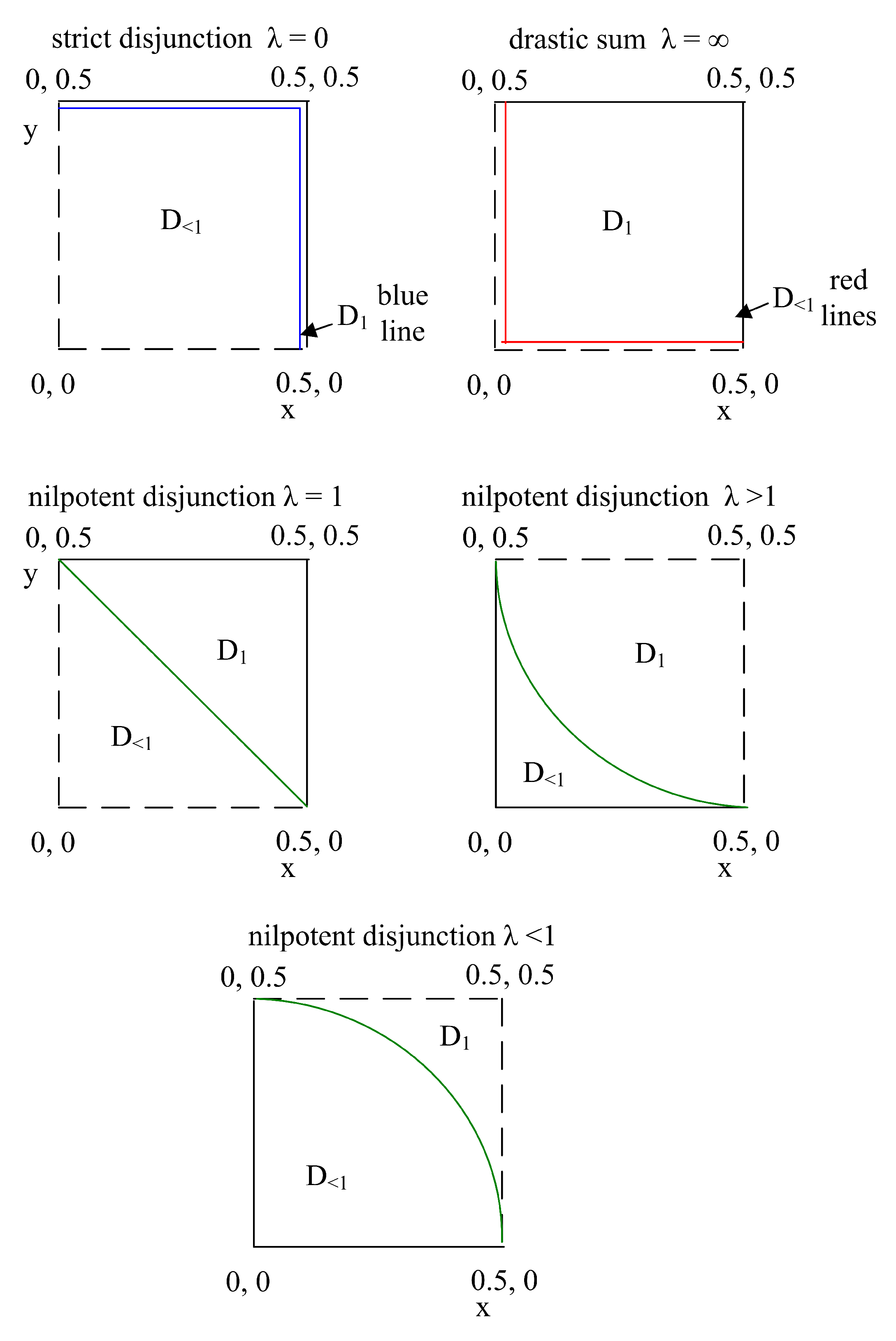
This family of t-conorms is remarkable in the sense that it contains all four basic t-conorms. Next, it covers the whole range of nilpotency, whereas the other families have nilpotency as a special case. We need nilpotency for flexible separation of the clear belonging to the class “yes”, see Figure 2. Due to the duality principle of aggregation functions, the same observation holds for class “no” (the nilpotency of conjunctive functions).
When we want to adapt Equation (7) to [ 0.5 , 1 ] 2 (see Figure 1), we obtain max ( x , y ) for λ = , 1 + 2 x + 2 y 2 x y for λ = 0 , max ( x , y ) if max ( x , y ) = 0.5 and 1 otherwise for λ = and 1 max ( 1 x + 1 y 0.5 ) for λ = 1 . Concerning the learning, in disjunctive subsquare (Figure 1) we obtain the following equation
D λ S ( x , y ) = 1 max ( 0 , ( 1 x ) λ + ( 1 y ) λ 0 . 5 λ ) 1 λ
for the values of λ ] 0 , [ . This is a theoretical limit, but for the learning process we limited values to 5, as learning large values is not suitable.
For λ = 0 , we obtain probabilistic sum t-norm, i.e., D 1 holds only when x = 1 or y = 1 for x , y [ 0.5 , 1 ] 2 , whereas the whole inner space and its left and lower bound belong to D < 1 . This case is depicted in Figure 2 upper left part. This is a solution when the domain expert wants a clear 1 in the case when one attribute is clearly ideal and another has a high satisfaction value. In the opposite case, when λ = we obtain the drastic sum, i.e., D 1 is everywhere except on dashed lines of [ 0.5 , 1 ] 2 in Figure 2 upper right part. We should avoid very high values of λ , because machine learning cannot efficiently cope with . While further optimisation in this direction is also promising for research, this work is focused on the learning of the separator between D 1 and D < 1 .
Next, adopting λ = leads to maximum t-conorm, which is not the right function due to the non-compensatory effect, i.e., E 1 ( 0.9 , 0.6 ) and E 2 ( 0.9 , 0.9 ) are indistinguishable [3].
When λ = 1 , we obtain the Łukasiewicz t-conorm, i.e, a separator is a diagonal line of the considered quadrant (see Figure 2 left part in second row), i.e., areas D 1 and D < 1 are of equal size. Naturally, the question is how to adjust this separation curve by parameter λ (Figure 2, fourth and fifth diagram).
The first option to adjust classification space is to graphically interpret positions of entities when λ = 1 and allow domain experts to mark each data point and indicate whether it should be in D 1 or D < 1 . In the next step, ML could find the most suitable non-linear separator (via the value of λ ). In this way, the domain expert explains the requirements for classification linguistically and consequently fine-tunes the resulting classification space. The second option is from the already classified data to compute the best value of λ to meet the acceptable accuracy. However, the problem is that entities are classified into binary classes or winner-takes-all; that is, entities are classified into classes with higher matching degrees. The analogous observation holds for the conjunctive part C 1 and C < 1 , where the solution is a family covering the whole range of nilpotency in a disjunctive function, i.e., parametrised Schweizer–Sklar family of t-conorms [47].
When we want to adapt Equation (10) to [ 0 , 0.5 ] 2 (see Figure 1) we obtain min ( x , y ) for λ = , 2 x y for λ = 0 , min ( x , y ) if min ( x , y ) = 0.5 and 0 otherwise for λ = and max ( x + y 0.5 ) for λ = 1 . Concerning the learning task, for the conjunctive subsquare (Figure 1) we have the equation:
C λ S ( x , y ) = ( max ( x λ + y λ 0 . 5 λ , 0 ) ) 1 λ
for the values of λ ] 0 , [ .
C λ S ( x , y ) = min ( x , y ) for   λ = D P ( x , y ) for   λ = 0 D D ( x , y ) for   λ = ( max ( ( x λ + y λ 1 , 0 ) ) 1 λ else
Classification into the class maybe is activated when one attribute has high value and another low value, i.e., IF A1 is high and A2 is low THEN B is maybe. The simplest solution is adopting a logically neutral averaging function, i.e., arithmetic mean. The other averaging functions are either conjunctively or disjunctively polarised [45]. Conjunctively polarised functions are further divided into soft ones (without an absorbing element) and hard ones (absorbing elements equal to 0, such as geometric mean, for instance). Analogously, disjunctively polarised averaging functions are divided into soft ones (without an absorbing element) and hard ones (absorbing elements equal to 1, such as dual geometric mean, for instance). Hence, the direction of polarisation should be learned from data and/or linguistically provided by a domain expert and fine-tuned from the subset of labelled data.
Averaging functions can be expressed by a power mean (a subclass of averaging function) as
M r ( x , y ) = 1 2 ( x r + y r ) ( 1 / r )
for r ] , [ , when r = 0 , M 0 ( x , y ) is geometric mean (proof for r 0 is in, e.g., [47]). This function is the borderline case between the hard and soft polarised conjunctive functions).
For r = 1 , we obtain the arithmetic mean (neutral behaviour). Thus, for r < 1 we have conjunctively polarised functions, whereas for r > 1 we obtain disjunctively polarised functions. The family of power means can be extended by the limiting cases:
M ( x , y ) = lim r M r ( x , y ) = min ( x , y )
M ( x , y ) = lim r M r ( x , y ) = max ( x , y )
For machine learning, the problem is working with and . However, functions MIN and MAX are not suitable due to the non-compensatory effect. The problem is dividing by zero (to obtain the behaviour of the geometric mean). It indicates conjunctive polarisation, G ( 0.3 , 0.7 ) = 0.46 < 0.5 . However, for G ( 0 , 0.9 ) we obtain 0. This solution is problematic. When we have expected rule IF A1 is small AND A2 is high THEN maybe, geometric mean classifies to a clear no. Thus, for seamless learning we should assign, e.g., r > 0 . In the case of Example 1, the range is r / i n ] 0 , 1 ] . On the other hand, due to the asymmetry of power mean and the existence of annihilator only for MAX, the acceptable range in disjunctive polarisation is in ] 1 , [ . For learning, this is inconvenient. Hence, we should limit the range to ] 1 , m [ in a way that when the result is not very close to m, the range is acceptable. Even though this works, the task for future research is searching for a function which covers similarity, because the known categorisation by power mean is not the ideal solution. These theoretical observations create rules for applying ML in learning parameters for classifying by ordinal sums as follows:
  • For data points in [ 0 , 0.5 ] 2 the ML model learns parameters for strict or nilpotent conjunction to classify into class no
  • For data points in [ 0.5 , 1 ] 2 the ML model learns parameters for strict or nilpotent disjunction to classify into class yes
  • For data points in [ 0 , 0.5 ] × [ 0.5 , 1 ] [ 0.5 , 1 ] × [ 0 , 0.5 ] the ML model learns parameters for power means to classify into class maybe
The next problem is classification by dissimilarities, i.e., when values of attributes are very similar or equal, the class is “irrelevant difference” (or 0); when values of attributes are very or fully dissimilar (or 1) the result is “key difference”. Otherwise, the result is class “partial difference” (in the open unit interval). The next section explores this problem and proposes a new dissimilarity function.

4. A New Dissimilarity Function for Classifying by XOR into Classes Yes, No and Maybe

The challenge is the fact that XOR is not an aggregation function. Conjunctions, disjunctions and averaging functions belong to the class of aggregation functions, i.e., functions A : [ 0 , 1 ] n [ 0 , 1 ] which are monotone and satisfy the boundary conditions A ( 0 , , 0 ) = 0 and A ( 1 , , 1 ) = 1 , n N . Observe that for XOR, F ( 1 , 1 ) = 0 holds.
The classical XOR cover cases when one of two attributes should be satisfied but not both. In two-valued logic X O R ( 0 , 0 ) = 0 , X O R ( 1 , 1 ) = 0 , X O R ( 1 , 0 ) = 1 , X O R ( 0 , 1 ) = 1 hold. In many-valued logic, this function is expressed as a dissimilarity function. The main obstacle is that XOR is not an aggregation function due to a violation of boundary conditions. Nevertheless, this function should keep monotonicity and satisfy the condition for the two-valued case. In this case, when levels of both attributes are medium (with values 0.5), the solution should be 0 or near 0 to indicate uncertainty, when values of attributes are neither high nor low. Employing the XOR problem might especially be useful for the study of technical batch effects influencing the measurement of molecular probes. Batch effects hinder a comprehensive comparison between healthy patients and, e.g., patients with a viral infection. In case two laboratory strategies produce different results (e.g., levels of antibodies) on the exact same molecular profile, an efficient comparison between patients or probes is difficult. Thus, laboratory strategies, even when they differ slightly, assure quality, as long as the quantified molecular quantities are on the same normalised scale (both high or both low).
Q D ( x , y ) = 0 , if [ x , y ] A 1 0 , if [ x , y ] A 2 1 , if [ x , y ] A 3 1 , if [ x , y ] A 4 x 1 2 s 2 p 1 1 + y 1 1 2 p 1 + s + s 2 p 1 1 , if [ x , y ] A 5 x 1 p 1 + p 1 + p 2 1 p 1 2 p 1 2 + y 1 1 2 p 1 p 2 1 2 p 1 , if [ x , y ] A 6 ( 1 x ) 1 2 s 2 p 1 1 + 1 y 1 2 p 1 + s + s 2 p 1 1 , if [ x , y ] A 7 ( 1 x ) 1 p 1 + p 1 + p 2 1 p 1 2 p 1 2 + 1 y 1 2 p 1 p 2 1 2 p 1 , if [ x , y ] A 8 y 1 2 s 2 p 1 1 + x 1 1 2 p 1 + s + s 2 p 1 1 , if [ x , y ] A 9 y 1 p 1 + p 1 + p 2 1 p 1 2 p 1 2 + x 1 1 2 p 1 p 2 1 2 p 1 , if [ x , y ] A 10 ( 1 y ) 1 2 s 2 p 1 1 + 1 x 1 2 p 1 + s + s 2 p 1 1 , if [ x , y ] A 11 ( 1 y ) 1 p 1 + p 1 + p 2 1 p 1 2 p 1 2 + ( 1 x ) 1 1 2 p 1 p 2 1 2 p 1 , if [ x , y ] A 12
where A 1 , , A 12 [ 0 , 1 ] × [ 0 , 1 ] are given by:
A 1 : x p 1 p 1 p 2 p 1 p 2 p 1 p 2 y x p 1 p 2 p 1 + p 2 A 2 : x p 1 p 2 p 1 + p 2 p 1 p 2 p 1 y x p 1 p 1 p 2 + p 1 p 2 p 2 p 1 p 2 A 3 : y x p 1 p 2 p 1 + 1 + p 2 2 p 1 & y x p 1 p 1 p 2 2 p 1 2 p 1 p 2 p 1 + p 2 p 1 p 2 A 4 : y x p 1 p 1 p 2 + 2 p 1 2 p 1 p 2 p 1 p 1 p 2 & y x p 1 p 2 p 1 + 2 p 1 2 p 1 p 2 p 1 + p 2 p 1 A 5 : p 1 x 1 2 & x y 1 x
A 6 : 0 x p 1 & x p 1 p 2 p 1 + p 2 y x p 1 p 2 p 1 + 1 + p 2 2 p 1 A 7 : 1 2 x 1 p 1 & 1 x y x A 8 : 1 p 1 x 1 & x p 1 p 2 p 1 + 2 p 1 2 p 1 p 2 p 1 + p 2 p 1 y x p 1 p 2 p 1 + p 2 p 1 p 2 p 1 A 9 : p 1 y 1 2 & y x 1 y A 10 : 0 y p 1 & y p 1 p 2 p 1 + p 2 x y p 1 p 2 p 1 + 1 + p 2 2 p 1 A 11 : 1 2 y 1 p 1 & 1 y x y A 12 : 1 p 1 y 1 & y p 1 p 2 p 1 + 2 p 1 2 p 1 p 2 p 1 + p 2 p 1 x y p 1 p 2 p 1 + p 2 p 1 p 2 p 1
In this classification, differences should be emphasised and similarities should be attenuated. In addition, the function should be monotonic. Generally, XOR is expressed as R ( x , y ) = | x y | . For two-valued logic, we obtain R ( 0 , 0 ) = 0 , R ( 1 , 0 ) = 1 , R ( 0 , 1 ) = 1 (due to similarity) and in general R ( x , x ) = 0 for all x [ 0 , 1 ] . When searching for flexibility in XOR or dissimilarity function, we should consider boundary conditions and monotonicity. Small deviation in data or non-full dissimilarity should be covered, i.e, R ( 0 , 98 , 0.01 ) = 1 . The same holds for the diagonal of the unit square from (0,0) to (1,1), which should theoretically keep the value 0 or at least in edges of the diagonal and near edges. The main diagonal solution should be 0. In the point (0.5, 0.5) and its vicinity we might assign a value greater than 0 (the value s = f ( 0.5 , 0.5 ) below) to indicate that when intensities of satisfaction are not high, a low dissimilarity exists. We introduce a new notion of quasi-dissimilarity function to keep this flexibility and propose a parametric class of quasi-dissimilarity functions.
For our intention, neither fuzzy XOR nor fuzzy dissimilarity is fully convenient since XOR requires associativity [25] (which is not important for us) and dissimilarity d should satisfy d ( x , x ) = 0 for all possible x [48] (while we do not have such strong demand—see discussion above). This observation led us to introduce a notion of fuzzy quasi-dissimilarity function.
Definition 1.
A function Q D : [ 0 , 1 ] × [ 0 , 1 ] [ 0 , 1 ] is a fuzzy quasi-dissimilarity function if it satisfies, for all x , y , z [ 0 , 1 ] , the properties:
  • (QD1) Q D ( x , y ) = Q D ( y , x ) ;
  • (QD2) Q D ( 1 , 0 ) = Q D ( 0 , 1 ) = 1 ;
  • (QD3) Q D ( 0 , 0 ) = Q D ( 1 , 1 ) = 0 ;
  • (QD4) Q D ( x , x ) Q D ( y , y ) whenever | x 0.5 | | y 0.5 | ;
  • (QD5) Q D ( x , y ) Q D ( x , z ) and Q D ( y , z ) Q D ( x , z ) whenever x y z .
It is worth putting out that the first, second and fifth properties are standard properties demanded from dissimilarity functions [28,49]. The third property is a relaxed version of the usually used D ( x , x ) = 0 for all x [ 0 , 1 ] . The fourth property is a new requirement of the monotonicity of function Q D on the main diagonal of the unit square.
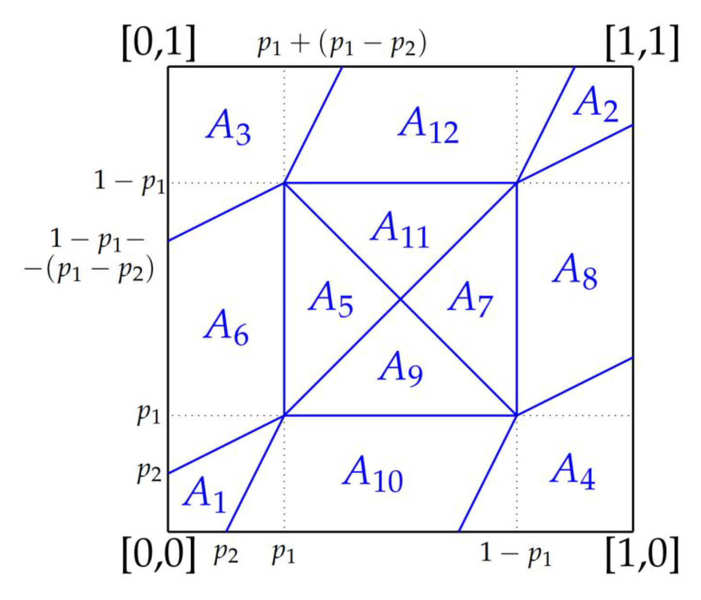
Now we construct a parametric class of fuzzy quasi-dissimilarity functions. Let us divide the unit square into 12 areas according to Figure 3 with the parameters:
  • s [ 0 , 1 ] , s = f ( 0.5 , 0.5 ) ;
  • p 1 [ 0 , 0.5 ] ;
  • p 2 [ 0 , p 1 [ .
It is also possible to take p 2 = p 1 , but in that case, the formula needs to be adjusted.
Then the function given by Equation (14) is a fuzzy quasi-dissimilarity function (see Figure 4 for an example of the function with the parameters s = 1 / 3 , p 1 = 1 / 4 and p 2 = 1 / 8 ).
Figure 3. The 12 areas of the unique square corresponding to Equation (14).
Make 04 00047 g003
Figure 4. The graph of the function Q D ( x , y ) given by Equation (14) for the parameters s = 1 / 3 , p 1 = 1 / 4 and p 2 = 1 / 8 .
Make 04 00047 g004
It is worth mentioning that taking s = 0 in Equation (14), the function Q D is a fuzzy dissimilarity function.
To evaluate the validity of the set of Equation (14), we have generated XOR-like data using gene expression values from patients suffering from kidney cancer. The data were retrieved from the Cancer Genome Atlas (https://www.cancer.gov/tcga accessed on 25 September 2022). We sampled two patients with similar phenotypic characteristics regarding age and smoking status. For these two patients, a total number of about 19,936 genes were available. We min-max normalised the expression values to a range of [ 0 , 1 ] . Following that, we calculated the absolute difference (Manhattan distance [50]) for each gene between the two patients. In the first investigation, we set an artificial threshold value of 0.5 . Differences in gene expression below that threshold were assigned with the label 1 (18,715 samples). The rest was labelled by the class 0 (1221 samples). The resulting XOR representation of the survival data allows a researcher to study the gene levels of single patient pairs and ultimately could help to detect biomarkers. This is particularly interesting for patients with similar medical characteristics. The causal force causing a death outcome may originate from a dysregulated gene function. Our XOR model may be used to explore such patterns and ultimately may help to detect novel biomarker genes.
Figure 5 depicts the original data, with inversed target value (the values of the target that were 0 were set to 1 and the ones that had the value 1 have now the value 0).
To search for adequate parameters p 1 , p 2 and s, an evolutionary algorithm was programmed in Python with the use of the library DEAP: https://deap.readthedocs.io/en/master/ (accessed on 25 September 2022). All figures were generated with the use of the plotly library https://plotly.com/ 25 September 2022. The parameterisation of the algorithm is the same as in Section 5.1.3. Added to that, the constraints p 1 [ 0 , 0.5 ] , p 2 [ 0 , p 1 [ , s [ 0 , 1 ] were implemented with the use of a penalty when the proposed p 1 , p 2 , s were distant from the region of feasible solutions. There were several combinations of p 1 , p 2 , s values that were a good local minimum; the approximated data depicted in Figure 6 are just one of them. The average value of the Mean Squared Error (MSE) of the discovered solutions w.r.t. the original XOR data was 0.046 for 10 independent runs.

5. Parameter Learning in Classification by Ordinal Sums with Evolutionary Algorithm and Reinforcement Learning

Parameter learning can be made reliably with the use of ordinal sums and evolutionary algorithms from real data [51,52]. We conducted two separate experiments with synthetically generated data; each of them containing 25 data samples created with the same pre-specified parameterisation and 4 with a slightly different perturbed version of the estimated parameter. The goal of the evolutionary algorithm is to estimate the original parameter from the perturbed data.

5.1. Parameter Learning for Conjunctive and Averaging Functions

For the learning, the input data are listed in Table 1 (for the conjunctive part of the classification space) and Table 2 (for the averaging part of the classification space, see Figure 1). Concerning the disjunctive part, it is dual to conjunctive and therefore is not examined.
The areas in Figure 1 can be roughly described by the following behaviour:
  • C 0 —Clear no
  • C > 0 —Very significant inclination to no
  • Avg—Averaging functions with possible inclination to no or yes
  • D < 1 —Very significant inclination to yes
  • D 1 —Clear yes

5.1.1. Averaging Behaviour for Class Maybe

The average function covers classification to class maybe when value of x is high and value of y is low and the opposite Figure 1. This function is managed by the power mean (Equation (11)) that generates the last column (the intensity to belonging to the class maybe) in Table 2.
Depending on the value of r, the following behaviour is expressed:
  • r = 1 : Neutral
  • r > 1 : Optimistic—A bit inclination to yes
  • 0 < r < 1 : Pessimistic—A bit inclination to no
Some examples of the output of function (11) on pairs of ( x , y ) variables:
( 0.3 , 0.7 ) 0.5 ( r = 1 ) ( 0.3 , 0.7 ) 0.58 ( r = 2 ) ( 0.3 , 0.7 ) 0.46 ( r = 0.5 )
Theoretically, r can be any value, whereas value 0 for the geometric mean is a special case. It cannot be learnt due to dividing by zero. The first solution is constraining learning to values in the interval ( 0 , 2 ) . This interval focuses on learning the so-called soft conjunctively and soft disjunctively polarised averaging functions. The second solution covers learning also hard conjunctively and hard disjunctively polarised functions (except for r = 0 ). These functions are examined in detail in [45]. Due to the internality principle of averaging functions, the solution is between the minimal and maximal value, but for the cases ( 0 , 1 ) the solution is 0 for the hard conjunctive polarisation and 1 for the hard disjunctive polarisation. This contradicts the classification into class maybe for a rule IF x is SMALL and y is HIGH THEN solution is MEDIUM.
An example of learning is shown in Table 2 where values indicate that classification (e.g., in Example 1) should be restrictive (a bit of inclination to class no, as domain expert indicated), whereas values marked as bold indicate that for these records classification has been recognised as neutral or optimistic. When we exclude these records, the solution is r = 0.75 . The influence of these records has increased the value of r towards the new learned value r = 0.88 . The results are depicted in Figure 7.

5.1.2. Conjunctive Behaviour for Class No

In this part of classification space, we should adjust the separation line (or curve) between C 0 and C > 0 , where
  • For area C > 0 : C L ( x , y ) > 0 and C L ( x , y ) < min ( x , y )
  • For area C > 0 : C ( x , y ) = 0
This classification is realised by the parametrised nilpotent family of conjunctive functions (10), i.e.,
  • λ = 1 : Linear case, i.e., ( 0.3 , 0.2 ) = 0
  • λ > 1 : More restrictive, for instance ( 0.3 , 0.4 ) = 0 , for λ = 2
  • λ < 1 : Less restrictive, for instance ( 0.3 , 0.2 ) = 0.1 , for λ = 0.1
An example of learning is shown in Table 1 where values indicate that classification into class no should contain a larger percentage of space, whereas values marked as bold indicate that for these records class no cover a smaller percentage of the classification space. When we exclude these records, the solution is λ = 1.25 . The influence of these records has decreased the value of λ towards the new learned value λ = 1.22 . The results are depicted in Figure 8.

5.1.3. Implementation of Parameter Estimation from Synthetically Generated Noisy Data with an Evolutionary Algorithm

The data that were used for the experiment for the averaging part are presented in Table 2. The data were in principle generated with r = 0.75 (more restrictive). For the marked records in red, r is different (two of them 1 and the other two 1.25 ). The evolutionary algorithm was implemented with the same software as the one mentioned in Section 4.
With an evolutionary algorithm, we search with the use of a population of 100 elements for the right r. The starting values should lie between ( 0 , 5 ) as was indicated above. However, when humans express a more restrictive classification of high and low values, the starting values lie between ( 0 , 1 ) and their starting distribution is uniform. The operators that are used are mating, mutation and selection. The mate probability was set to 0.5 ; the mutation Gaussian distribution has a mean equal to 0.0 and a standard deviation of 1.0 . The mutation probability was set to 0.2 . Those values were defined after several executions of the algorithm to provide the best possible mean squared error (MSE) between the original and estimated function. The number of generations that were needed for a satisfying result was 100 and the solution is computed in approximately 40 s even without parallelism. There were some edge cases that one needs to consider, such that during the evolutionary algorithm the r in 1 / r might take the value of zero or that in the averaging case Python does not raise a negative number to a fractional power.
The same observation holds for learning parameters for the conjunctive part, except for the different functions used. In the above experiment, the estimated value of λ is 1.25 . The size of the dataset depends on the number of outliers and on the data distribution to cover the whole domain.

5.1.4. Implementation of Parameter Estimation from Synthetically Generated Noisy Data with Reinforcement Learning

The estimation problem described in Section 5.1.3 can also be solved with the use of a reinforcement learning algorithm [53,54,55]. Although this might seem a too complex method for the solution of such a task, it is expected that for more sophisticated estimations with many more parameters and higher dimensionality, it can be proven beneficial.
As with every basic reinforcement learning algorithm, the first step was to define the environment and the agent; the environment does not consist of a known Markov Decision Process (MDP). The episode can terminate either when the number of maximum steps is reached or when the mean squared error (MSE) between the original and the estimated function is less than a predefined threshold (just as in the case of the evolutionary algorithm in the previous Section 5.1.3). The reward strategy can be either the minimum time to goal or one that is less discouraging and equal to the minus of the currently computed MSE. The agent’s states are all float numbers in the x axis between 0 and 1 (bounds that are provided by the problem definition and can be adapted). The permissible actions can move the agent either left or right in this axis by a small amount each time (currently set to 0.01 ).
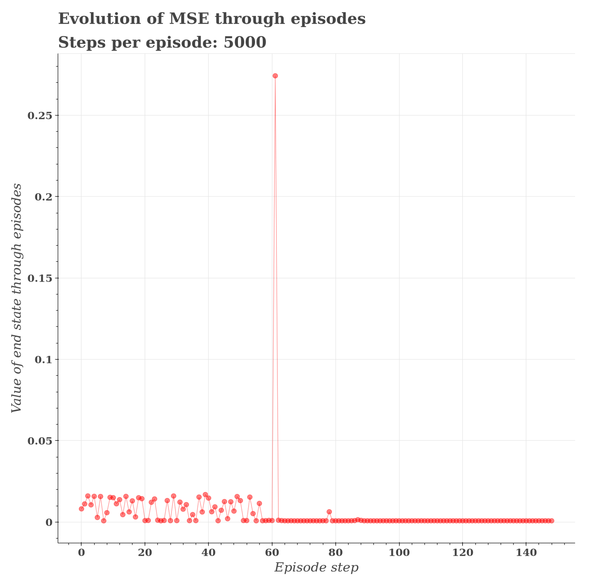
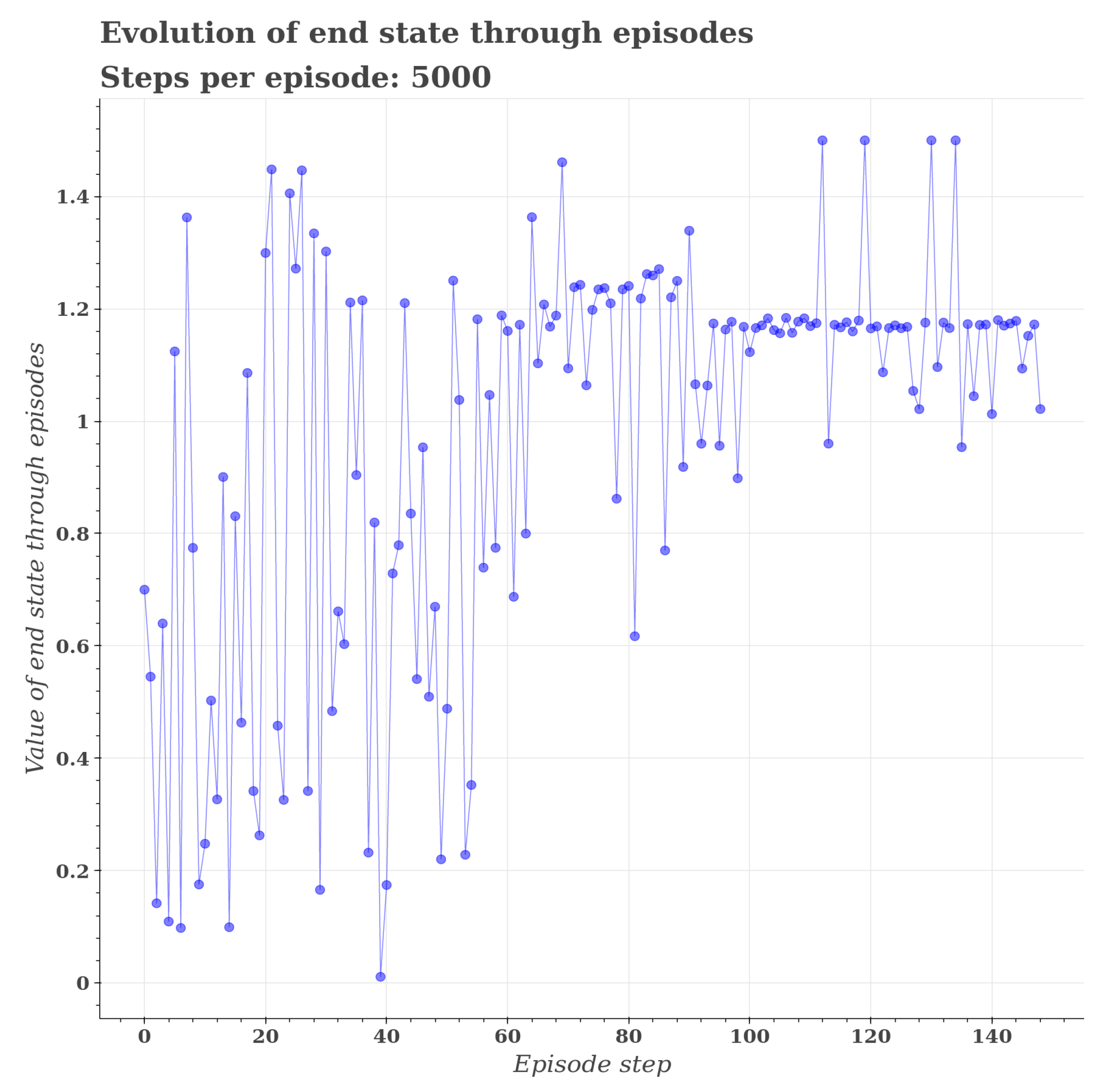
We implemented a custom environment and the agent with the following Python library: https://mushroomrl.readthedocs.io/en/latest/ (accessed on 25 September 2022). The reinforcement learning algorithm was used as the True online TD (lambda) [56]; since we do not have a defined MDP, we could also use a Deep Q-Network [57] in a more complex estimation problem. We tried two rewarding schemes; the use of the minus of the MSE to the solution and the minimum time to goal; the second one has proven not to converge in a reasonable time duration. We have tried several combinations of numbers of episodes and maximum steps per episode and the smallest one that provided us results comparable to the evolutionary algorithm for the averaging function was 150 and 5000, respectively. As one can see in Figure 9, the last state that the agent finds himself at the end of the episode converges to a value 0.87 and the same goes for the MSE, as shown in Figure 10.
The search for the appropriate parameter for the conjunctive function follows the same pattern. After the exploration phase, the agent finds the solution near 1.2 at the end of each episode, as seen in Figure 11 and Figure 12.

6. Experiment on Medical Data for Classification by Ordinal Sums

Medical data are valuable support for medical doctors when they can easily analyse them. In this section, the Cleveland Heart Disease dataset from the dataset repository of the University of California, Irvine (UCI) [58], is used. This dataset related to heart issues is an established real-world dataset that is largely used in the machine learning field [59,60,61]. The classification space is created in a way that medical doctors can adjust parameters intuitively. This section contains an example of such a process with the use of a novel tool to explore prepared datasets. This tool expects datasets in a comma-separated values (CSV) format and can theoretically be used for a wide variety of data. For this experiment, though, the application has been primarily programmed to visualise the diagnosis of each patient of the dataset described in Section 6.1 and compare it to the resulting distribution of the data points on a two-dimensional plot.

6.1. Dataset Information

The dataset was derived from clinical and non-invasive test results from 303 patients at the Cleveland Clinic in Cleveland, Ohio [62]. It contains 14 features, 4 of them being clinical attributes and the rest attributes gathered from clinical tests on the patient.
Clinical attributes are age, sex (0 = female, 1 = male), chest pain type and blood pressure. Chest pain type is further segregated into typical angina (angina pectoris), atypical angina, non-anginal pain and no pain (asymptomatic), which have the identifiers 1, 2, 3 and 4, respectively. Studies have shown that patients with typical angina are more likely to suffer from coronary disease while other types of pain do not give any indications toward this disease in general [63,64].
The remaining attributes were gathered during non-invasive tests. The resting electrocardiograph results are divided into three categories: normal results, results with ST-T wave abnormality and apparent left ventricular hypertrophy by Estes’ criteria. Similarly, there was an exercise electrocardiogram, but in this case, the maximum achieved heart rate was recorded. Obtaining good limits for this attribute is rather difficult. The measure for a value to be considered good depends on the age of the patient [65]. Generally, a higher value indicates a healthier patient. The limits chosen for this attribute are an educated guess based on prior research [66]. ST segment depression was recorded by comparing it to the resting baseline and is measured in mV. The slope of the ST segment peak was recorded as either upsloping, flat or downsloping and marked by the identifiers 1, 2 and 3, respectively. Lastly, thallium scintigraphic defects were recorded as either normal, fixed defects or reversible defects by the values 3, 6 and 7 in that order. Further attributes are serum cholestoral, fasting blood sugar (0 if ≤ 120 mg/dL, otherwise 1), exercise induced angina (0 = no, 1 = yes) and fluoroscopy for coronary calcium.
Finally, there is an attribute for the presence of heart disease. At value 0 there is an absence of disease in this patient and values 1–4 indicate a diameter narrowing larger than 50 % in at least one major blood vessel and thus a presence of heart disease.
It is noteworthy that the dataset contains six patients where the value for at least one of the attributes is missing. In the case of this experiment, these entries were simply removed from the dataset instead of substituting these values by using an average or assigning a random value (imputation), [67]. Thus the number of remaining patients in the used dataset amounts to 297.

6.2. Data Preprocessing

This application supports CSV files with a comma (“,”) as a separator. The first two lines of each CSV dataset are reserved for further information on the data for the tool to process. The first line of the file must contain all attribute names of the dataset in the structure A 1 , A 2 , , A n .
The second line must contain the limits of the attribute in the structure D L 1 | D H 1 , D L 2 | D H 2 , , D L n | D H n . The minimum ( D L i ) and maximum ( D H i ) limits of each attribute will be normalised to [0, 1] in the application. For the dataset from Section 6.1, these limits were defined as described in Table 3. For medical features, we assign value 0 to all values lower than or equal to D L and value 1 for values greater than or equal to D H when increasing means concern (above the value of D H is a full concern) and the opposite when decreased value means increased concern. For instance, the limit for the attribute thalach is given as [160, 120] which in this case simply means normalisation is inverted so that a value above 160 results in a 0 and a value below 120 results in a 1. The attribute age has a limit of [40, 65] in our dataset. However, when a new entity below 40 or above 65 is recorded, it does not simply mean that these values obtain values 0 or 1, respectively. New values of age adjust D L and D H . The remaining lines contain a patient entry each with all of their attribute values filled in the structure P A 1 , P A 2 , , P A n . Missing values are not supported and rows containing them have to be removed before being able to use the CSV file.
Generally, atomic attributes can be aggregated to a compound one in diverse ways. A convenient option is an aggregation by the fuzzy quantifier most of [68]. For instance, the most of declared distances in Example 1 should be short. In the medical domain, we cover cases when most of the symptoms belonging to the category should be met. The intensity of a quantified sentence indicates seriousness. More about the quantifier most of and its formalisation is in, e.g., [69].
The true value of the quantified sentence adapted to the evaluation of atomic attributes by the quantifier most of is expressed as
v ( x ) = μ Q 1 n i = 1 n μ P i ( x ) ,
where n is the number of atomic attributes, μ P i formalises the satisfaction of predicate P for the ith attribute and μ Q formalises quantifier most of as
μ Q ( y ) = 1 , f o r y n , y m n m , f o r m < y < n , 0 , f o r y m
where y is the proportion of satisfied atomic attributes, m and n are parameters expressing the strength of the quantifier.
For this quantification, the values m and n have to be set.

6.3. Tool Navigation

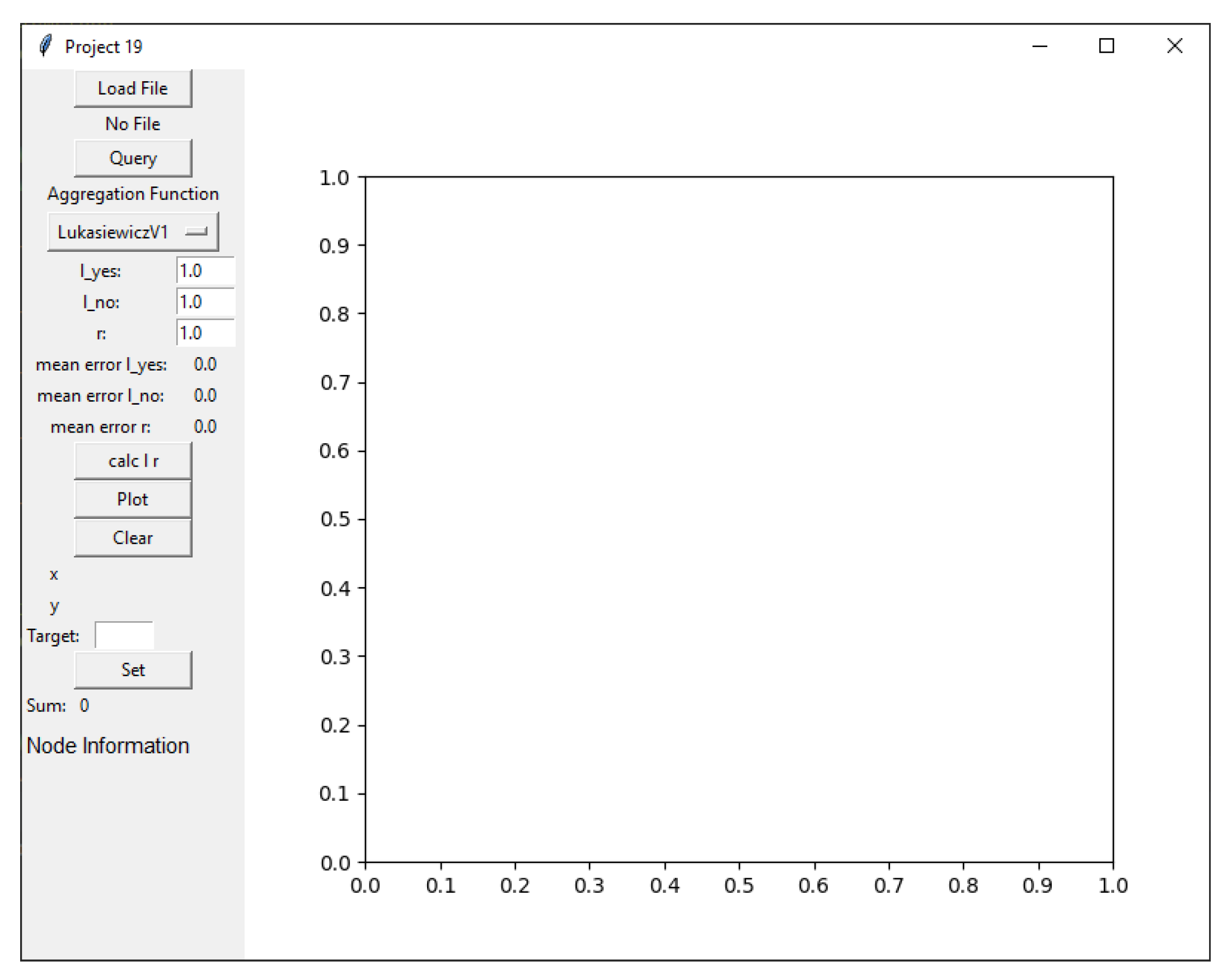
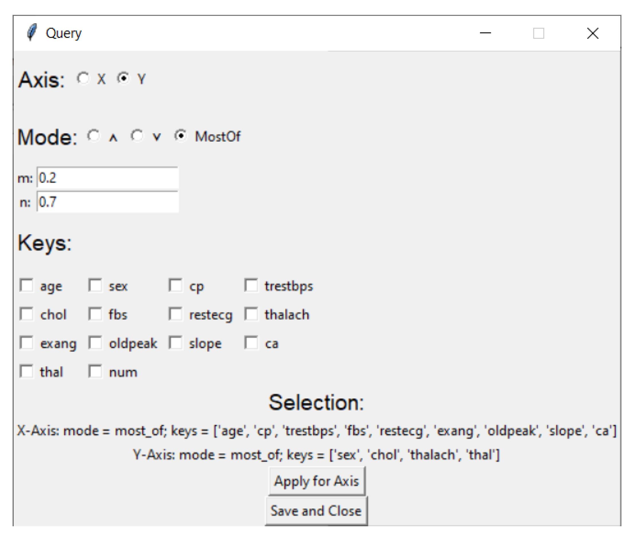
The interface of the custom application where the experiments and data exploration are performed is shown in Figure 13. Initially, a dataset as described in Section 6.2 needs to be loaded using the “Load File” button. When a file is loaded the “Query” button can be clicked in order to open the query window as seen in Figure 14. Within this window, the quantifier functions for the x and y axis can be defined by selecting the target axis, choosing an aggregation of atomic attributes (conjunctive or most of), selecting the target attributes from the dataset for the axis and clicking the “Apply for Axis” button. In case of most of quantifier, the parameters m and n need to be provided. The “Save and Close” button will then apply the settings and close the query window.
Now the “Plot” button can be clicked to plot the data. Using the parameters from Section 6.4 and the dataset as described above will then result in a plot seen in Figure 15. The user can then select a node by clicking on it, which displays information about the node in the “Node Information” field of the application. With a selected node, the target outcome value of the aggregation function can be defined by entering it into the “Target” input box and clicking the “Set” button. Providing the Cleveland Heart Disease dataset with the num attributes allows the application to preset the target values to 1 for patients with heart disease and 0 for patients without the disease. Additionally, nodes will be coloured based on the num attribute (0 = white, 1 = purple, 2 = green, 3 = blue, 4 = black).
Finally, using the “calc l r” button calculates a best match for the parameters λ and r. Note that for λ there are two separate input fields for the yes and no sections, respectively. The only prerequisite for obtaining a result from the “calc l r” button that differs from the default values is to have set at least one node to a target. After calculating those parameters, the labels “mean error l yes”, “mean error l no” and “mean error r” indicate mean error for each node with a target value.

6.4. Fitting Parameters

Defining parameters for the classification space is a challenging task. Usually, a domain expert can provide information in short sentences on how to quantify the data (e.g., Example 1). However, due to the lack of a domain expert, an automated way to define the parameters was used. For future and more complex tasks, we plan to include human-in-the-loop for explaining classification, validation and fine-tuning. The classification space was split into fields as shown in Figure 16. The goal was to fit as many patients into the correct classification as possible. The heart-disease-positive patients should be in the upper right half, while heart-disease-negative patients are expected in the bottom left area. To classify the nodes, a brute force approach was applied. For all possible subsets of attributes for the x and y axis, all possible values for m and n with a granularity of 0.1 were tested. For each possible parameter set, the number of nodes in the correct field was counted and the best overall score was used. In our experiment, we obtain the following values for quantifier most of (17) and compound attributes on axes:
  • m: 0.2
  • n: 0.7
  • x axis: [age, cp, trestbps, fbs, restecg, exang, oldpeak, slope, ca]
  • y axis: [sex, chol, thalach, thal]
Figure 16. Separation of the classification space for parameter fitting. The dataset from Section 6.1 is loaded in order to visualise the distribution of the points relative to the separator.
Make 04 00047 g016

6.5. Adjusting λ and r

The Schweizer–Sklar family of t-norms and t-conorms in ordinal sum require a parameter λ , whereas parameter r is required for the averaging functions, as described in Section 3. These parameters can be adjusted by the user to modify the strictness of the yes/no ( λ ) and the maybe (r) section. For example, if there are many data points in the no section that the user knows should be a definitive no (0), but are not classified as such, then the parameter λ of the no section can be increased to make the no section more inclusive and thus include these points. Similarly, the maybe section can be adjusted to tend more to no by decreasing the parameter r to indicate that data points near the no section within the maybe section lean more to a no decision. The same holds vice versa: To adjust the inclination in the other direction, the parameter r and λ of the yes section can be increased to alter the yes and maybe sections, respectively.
λ adjusts the strictness of the yes and no classifications. This enables the user to include or exclude data points inside the sections. The strictness of the yes and no sections can be independent of each other. The parameter r affects the strictness of the maybe classification. This leads to an inclination in the direction of the yes and no classifiers within the averaging class.

6.6. Interpretation of the Visualisation

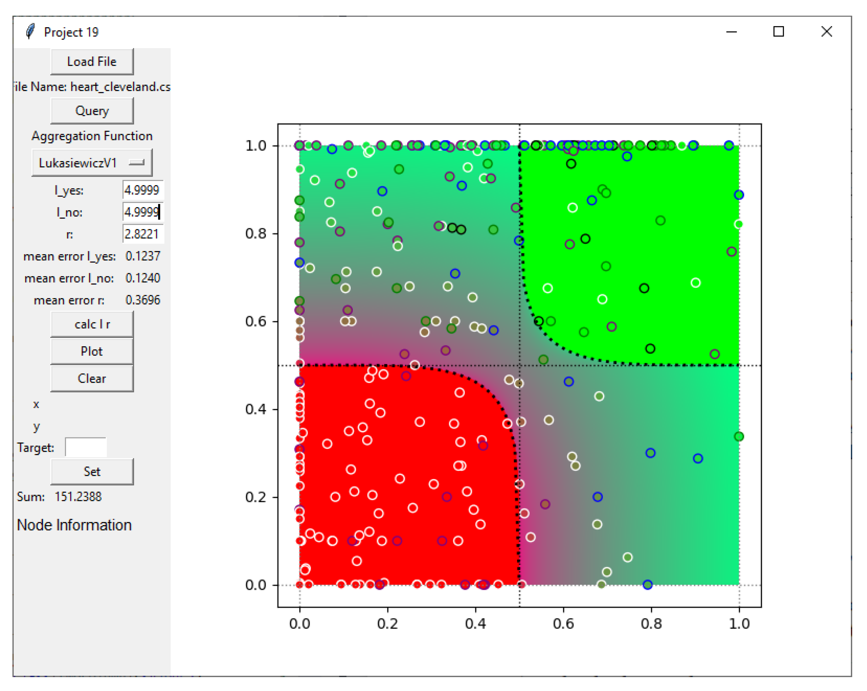
The aim is to achieve appropriate interaction between humans and data, so special care must be taken with visualisation to improve interactive processes [70]. Plotting the data without modifying the λ and r value results in a default value of 1 for these parameters. The plot for the example data described in Section 6.1 and quantified as explained in Section 6.4 can be seen in Figure 15. From this point on, the human-in-the-loop is essential to influence the classification [71]. Of course, the parameters λ and r can be manually set by the user, but a more intuitive way is for the domain expert to select data points within the plot and assign them to the yes or no class explicitly. After a moderate amount of assignments into both classes, the parameters can be trained by the tool and will yield a sensible adjustment to the strictness of the disjunctive, conjunctive and averaging classification. The resulting plot of the aforementioned data and set parameters results in the visualisation seen in Figure 17.
The colour coding as described in Section 6.3 assisted with the interpretation of the data. Naturally, there are some false positives and false negatives in the no and yes classes, respectively, but overall the classification of the data points within the yes and no class can be seen clearly.
Data points within the maybe classes require additional attention as these are interesting cases which do not have a clear yes or no answer to them and require further investigation by the user or domain expert. In the case of the Cleveland Heart Disease dataset, the number of patients in this category is quite high as humans react and develop symptoms very differently. Overall, the tendency for a data point to align with the overall correctness of identifying the disease is there. The outcome of the classification space is shown in Table 4.

7. Discussion and Future Works

By the concepts of aggregation functions (ordinal sums of conjunctive and disjunctive functions) for classification space, quantified and conjunctive aggregation for the atomic attributes and flexible XOR, we are able to perform classification tasks and moreover explain the result by functions and also linguistically.
In [3], we solved the classification task when the requirement is explained linguistically by a paragraph instead of rules. In this work, we have shown that, when we have a subset of data, for which we know to which class they belong, we are able to adjust parameters of nilpotency for the Schweizer–Sklar family of t-norms and t-conorms.
Next, we learned parameters for nilpotent conjunctive and disjunctive functions as well as the most suitable aggregation of atomic attributes into two compound ones. We obtain similar results as expected for classifying heart disease data. There is still space for improvement, but this is the first attempt to realise classification by ordinal sums on real-world data without domain expert intervention. The solution is interpreted graphically and interactively. The former means that when the domain expert move classified items inside the classification square, the new linear or non-linear separator between classes (parameter λ ) is learnt. The next task is to include human-in-the-loop (domain expert) especially for less frequently occurring events to explain classification tasks linguistically, learn separators of classes from a smaller subset of already classified data and allow a domain expert to adjust data positions in classification space and consequently fine-tune the classification space.
In our experiment, we explained classification space by a curve, which separates classes no and maybe, which is expressed by function (18):
T λ S ( x , y ) = ( max ( 0 , x 4.9999 + y 4.9999 0 . 5 4.9999 ) ) 1 4.9999
The class maybe and its inclination to yes or no is explained by the power mean:
M r ( x , y ) = ( 1 2 ( x 2.8221 + y 2.8221 ) ) 1 2.8221
Finally, class yes and its separation with class maybe is expressed by:
S λ S ( x , y ) = 1 ( max ( 1 , ( 1 x ) 4.9999 + ( 1 y ) 4.9999 0 . 5 4.9999 ) ) 1 4.9999
The value r in the averaging function for class maybe indicates inclination to class yes. It is a desirable solution because it is a better option to put a false alarm and indicate that the patient should be further examined than to indicate that the patient inclines to a healthy state despite quite significant values of attributes. For classes yes and no, the parameter λ obtains high values, which indicates that the respective quadrants almost fully cover clear yes and no, respectively. The future task should be also focused on the flexibility of the parameter in an ordinal sum which separates three classes.
This classification is not easily compared with the other approaches because it covers the class maybe. Existing approaches are usually binary or winner takes all (entity belongs to class with the highest matching degree). Nonetheless, the inclination is a valuable insight into data and an inclination to binary classes for a domain expert. Furthermore, the domain expert can interfere by providing a linguistic explanation of the classification space, which is contextual and sometimes also person-dependent (whether comfort is more or less relevant than distance).
The interpretability of black-box approaches can be mitigated by a transparent model with the aim of imitating the output of a black box, which is taken as an oracle, whereas a transparent model is a surrogate model [5]. From the experiment, we conclude that the proposed classification by ordinal sums and aggregating atomic conditions by quantified aggregation are suitable for this task, but further research is advisable.
In the classification by rule-based systems, neural networks, decision trees and the like, the entity is assigned to one class (in the case of fuzzy classification, the winner takes all or the entity is not classified). In the binary classification to classes yes and no, for many entities, this decision is not as simple as it looks at first sight. The option is to adopt classification into three classes, where belonging to the class maybe is clear for the remaining entities. However, for such entities domain experts would welcome information about the tendency towards the classes yes or no. It might be solved by additional classes like Tendency to no, Tendency to yes, which leads to the four-class classification. It adds flexibility but is still limited. In this approach, we have the clear belonging to classes yes and no for entities where the decision is clear and for all other entities we indicate the intensity of belonging to the class maybe. As intensity is lower, the entity inclines to class no. In the case of value 0.5, an entity has no inclination.
Upcoming future work is about learning parameters for the proposed dissimilarity function expressing flexible XOR for classification into three classes.

8. Conclusions

In many application areas, both experts and laypersons classify entities into binary classes (yes-no), e.g., healthy–sick, malignant–benign, credit accepted–rejected, etc.). However, for many entities, this decision is not as simple as it looks at first sight. In many cases, we need another class that can be labelled maybe, supported by a corresponding inclination towards one of these two extreme poles. Classification by ordinal sum of conjunctive and disjunctive behaviour is a new research field which is able to solve these requirements.
In our work, we developed a method for learning parameters of nilpotent t-norms and t-conorms and averaging functions from data. These parameters separate (linearly or non-linearly) three classes. Classification by two atomic or compound classifications is graphically interpretable. Thus, a domain expert is able to move entities into the desired classes or adjust inclination to one of two extreme poles. This information is input for re-learning and fine-tuning the classification space. Classification is demonstrated on the Cleveland Heart Disease dataset with a promising result. Accuracy can be improved by including human-in-the-loop in explaining requirements and fine-tuning.
The proposed classification approach is beneficial when requirements are expressed linguistically, the expert knowledge is not available in the form of rules, a labelled dataset is available or the labelled dataset has a smaller size, but the domain expert provides details relevant for recognising the sub-domains of parameters, e.g., the information about the tendency to be classified into class maybe. The proposed approach leads to an explainable and actionable AI solution.
The classification into class maybe requires further research as power means does not ideally cover soft conjunctive and soft disjunctive parts to apply ML. Further research in this direction is highly advisable to answer these observations. For future tasks, we also consider classification into several classes covering class “maybe”, to maintain the full belonging to one of the classes such as: “significant inclination to no”, “neutral inclination” and so forth.
The classification should be consistent, reliable and explainable. These three requirements are met by the proposed approach.
Next, we proposed the XOR classification into classes: “key difference”, “irrelevant difference” and “partial difference”. The novelty in comparison to the existing literature is the new dissimilarity function. Neither fuzzy XOR nor fuzzy dissimilarity is fully convenient, because we do not need a strong demand. A smaller deviation in the data (e.g., due to noise) should be handled. To solve this task, we introduced a fuzzy quasi-dissimilarity function and applied it on real-world data. The data that were used fulfil the XOR functional characteristics and both evolutionary algorithms as well as reinforcement learning can help us find adequate parameters that fit the data in a feasible region.

Author Contributions

All authors contributed to the writing of this manuscript. In particular, A.S. was responsible for conceptualisation, review and guiding software development and evaluation; M.H. contributed with conceptualisation, methodology, investigation, data analysis and theory development. E.M. contributed with data analysis, review and evaluation. Z.T. contributed with theory, evaluation and review; U.G. and C.K. contributed with software development, experiments and evaluation; B.P. contributed with evaluation and software analysis; A.H. contributed with conceptualisation, investigation, review and funding acquisition and acts as the corresponding author. Writing—review and editing, A.A.; Conceptualization, investigation, Writing—review and editing, A.H.; All authors have read and agreed to the published version of the manuscript.

Funding

Parts of this work have been funded by the Austrian Science Fund (FWF), Project: P-32554 “explainable Artificial Intelligence”.

Data Availability Statement

All code and data are openly available to the international research community via https://github.com/asaranti/Miroslav_Playground (accessed on 25 September 2022).

Acknowledgments

This work has been supported by the Austrian Science Fund (FWF), Project: P-32554 explainable Artificial Intelligence. Partial support of the KEGA No. 025EU-4/2021 project of the Ministry of Education, Science, Research and Sport of the Slovak Republic.

Conflicts of Interest

The authors declare no conflict of interests. This work does not raise any ethical issues.

References

  1. Bartoszuk, M.; Gagolewski, M. T-norms or t-conorms? How to aggregate similarity degrees for plagiarism detection. Knowl.-Based Syst. 2021, 231, 107427. [Google Scholar] [CrossRef]
  2. Patricia, M.; Daniel, S. Optimal design of type-2 fuzzy systems for diabetes classification based on genetic algorithms. Int. J. Hybrid Intell. Syst. 2021, 17, 15–32. [Google Scholar]
  3. Hudec, M.; Minarikova, E.; Mesiar, R.; Saranti, A.; Holzinger, A. Classification by ordinal sums of conjunctive and disjunctive functions for explainable AI and interpretable machine learning solutions. Knowl. Based Syst. 2021, 220, 106916. [Google Scholar] [CrossRef]
  4. Zadeh, L.A. Fuzzy logic = computing with words. IEEE Trans. Fuzzy Syst. 1996, 4, 103–111. [Google Scholar] [CrossRef] [Green Version]
  5. Alonso, J.M.; Castiello, C.; Magdalena, L.; Mencar, C. Explainable Fuzzy Systems; Springer: Cham, Switzerland, 2021. [Google Scholar]
  6. Wei, Z.; Man, L.; Zeshui, X.; Herrera-Viedma, E. Global fusion of multiple order relations and hesitant fuzzy decision analysis. Appl. Intell. 2021, 52, 6866–6888. [Google Scholar] [CrossRef]
  7. Arrieta, A.B.; Díaz-Rodríguez, N.; Del Ser, J.; Bennetot, A.; Tabik, S.; Barbado, A.; García, S.; Gil-López, S.; Molina, D.; Benjamins, R.; et al. Explainable Artificial Intelligence (XAI): Concepts, taxonomies, opportunities and challenges toward responsible AI. Inf. Fusion 2020, 58, 82–115. [Google Scholar] [CrossRef] [Green Version]
  8. Murray, B.; Anderson, D.T.; Havens, T.C. Actionable XAI for the Fuzzy Integral. In Proceedings of the IEEE International Conference on Fuzzy Systems (FUZZ-IEEE), Virtual, 11–14 July 2021; pp. 1–8. [Google Scholar] [CrossRef]
  9. Zhou, J.; Gandomi, A.H.; Chen, F.; Holzinger, A. Evaluating the Quality of Machine Learning Explanations: A Survey on Methods and Metrics. Electronics 2021, 10, 593. [Google Scholar] [CrossRef]
  10. Holzinger, A.; Saranti, A.; Molnar, C.; Biececk, P.; Samek, W. Explainable AI Methods - A Brief Overview. In XXAI-Lecture Notes in Artificial Intelligence LNAI 13200; Springer: Berlin/Heidelberg, Germany, 2022. [Google Scholar] [CrossRef]
  11. Shehab, M.; Abualigah, L.; Shambour, Q.; Abu-Hashem, M.A.; Shambour, M.K.Y.; Alsalibi, A.I.; Gandomi, A.H. Machine learning in medical applications: A review of state-of-the-art methods. Comput. Biol. Med. 2022, 145, 105458. [Google Scholar] [CrossRef]
  12. Holzinger, A.; Saranti, A.; Angerschmid, A.; Retzlaff, C.O.; Gronauer, A.; Pejakovic, V.; Medel, F.; Krexner, T.; Gollob, C.; Stampfer, K. Digital Transformation in Smart Farm and Forest Operations needs Human-Centered AI: Challenges and Future Directions. Sensors 2022, 22, 3043. [Google Scholar] [CrossRef]
  13. Hoenigsberger, F.; Saranti, A.; Angerschmid, A.; Retzlaff, C.O.; Gollob, C.; Witzmann, S.; Nothdurft, A.; Kieseberg, P.; Holzinger, A.; Stampfer, K. Machine Learning and Knowledge Extraction to Support Work Safety for Smart Forest Operations. In Proceedings of the International Cross-Domain Conference for Machine Learning and Knowledge Extraction, Vienna, Austria, 23–26 August 2022; pp. 362–375. [Google Scholar] [CrossRef]
  14. Holzinger, A.; Stampfer, K.; Nothdurft, A.; Gollob, C.; Kieseberg, P. Challenges in Artificial Intelligence for Smart Forestry. Eur. Res. Consort. Informatics Math. (ERCIM) News 2022, 130, 40–41. [Google Scholar]
  15. Holzinger, A. The Next Frontier: AI We Can Really Trust. In Proceedings of the ECML PKDD 2021, CCIS 1524, Bilbao, Spain, 13–17 September 2022; Kamp, M., Ed.; Springer Nature: Berlin/Heidelberg, Germany, 2021; pp. 427–440. [Google Scholar] [CrossRef]
  16. Krizhevsky, A.; Sutskever, I.; Hinton, G.E. Imagenet classification with deep convolutional neural networks. Commun. ACM 2017, 60, 84–90. [Google Scholar] [CrossRef] [Green Version]
  17. Araújo, T.; Aresta, G.; Castro, E.; Rouco, J.; Aguiar, P.; Eloy, C.; Polónia, A.; Campilho, A. Classification of breast cancer histology images using convolutional neural networks. PLoS ONE 2017, 12, e0177544. [Google Scholar] [CrossRef]
  18. Esteva, A.; Kuprel, B.; Novoa, R.A.; Ko, J.; Swetter, S.M.; Blau, H.M.; Thrun, S. Dermatologist-level classification of skin cancer with deep neural networks. Nature 2017, 542, 115–118. [Google Scholar] [CrossRef]
  19. Burt, J.R.; Torosdagli, N.; Khosravan, N.; RaviPrakash, H.; Mortazi, A.; Tissavirasingham, F.; Hussein, S.; Bagci, U. Deep learning beyond cats and dogs: Recent advances in diagnosing breast cancer with deep neural networks. Br. J. Radiol. 2018, 91, 20170545. [Google Scholar] [CrossRef]
  20. Stoeger, K.; Schneeberger, D.; Kieseberg, P.; Holzinger, A. Legal aspects of data cleansing in medical AI. Comput. Law Secur. Rev. 2021, 42, 105587. [Google Scholar] [CrossRef]
  21. French, R.M. Catastrophic forgetting in connectionist networks. Trends Cogn. Sci. 1999, 3, 128–135. [Google Scholar] [CrossRef]
  22. Novak, R.; Bahri, Y.; Abolafia, D.A.; Pennington, J.; Sohl-Dickstein, J. Sensitivity and generalization in neural networks: An empirical study. In Proceedings of the International Conference on Learning Representations, ICLR 2018, Vancouver, BC, Canada, 30 April–3 May 2018. [Google Scholar]
  23. Stoeger, K.; Schneeberger, D.; Holzinger, A. Medical Artificial Intelligence: The European Legal Perspective. Commun. ACM 2021, 64, 34–36. [Google Scholar] [CrossRef]
  24. Holzinger, A.; Mueller, H. Toward Human-AI Interfaces to Support Explainability and Causability in Medical AI. IEEE Comput. 2021, 54, 78–86. [Google Scholar] [CrossRef]
  25. Bedregal, B.C.; Reiser, R.H.; Dimuro, G.P. Xor-implications and E-implications: Classes of fuzzy implications based on fuzzy Xor. Electron. Notes Theor. Comput. Sci. 2009, 247, 5–18. [Google Scholar] [CrossRef] [Green Version]
  26. Mesiar, R.; Kolesarova, A.; Komornikova, M. Aggregation Functions on [0, 1]. In Springer Handbook of Computational Intelligence; Kacprzyk, J., Pedrycz, W., Eds.; Springer: Berlin/Heidelberg, Germany, 2015; pp. 61–74. [Google Scholar]
  27. Couso, I.; Garrido, L.; Sánchez, L. Similarity and dissimilarity measures between fuzzy sets: A formal relational study. Inf. Sci. 2013, 229, 122–141. [Google Scholar] [CrossRef]
  28. Bustince, H.; Mesiar, R.; Fernandez, J.; Galar, M.; Paternain, D.; Altalhi, A.; Dimuro, G.; Bedregal, B.; Takáč, Z. d-Choquet integrals: Choquet integrals based on dissimilarities. Fuzzy Sets Syst. 2021, 414, 1–27. [Google Scholar] [CrossRef]
  29. Kuncheva, L. Fuzzy Classifier Design; Physica-Verlag: Berlin/Heidelberg, Germany, 2000. [Google Scholar]
  30. Holzinger, A.; Plass, M.; Kickmeier-Rust, M.; Holzinger, K.; Crişan, G.C.; Pintea, C.M.; Palade, V. Interactive machine learning: Experimental evidence for the human in the algorithmic loop. Appl. Intell. 2019, 49, 2401–2414. [Google Scholar] [CrossRef] [Green Version]
  31. Lippmann, R.P. Pattern classification using neural networks. IEEE Commun. Mag. 1989, 27, 47–50. [Google Scholar] [CrossRef]
  32. Kohonen, T. Self-organized formation of topologically correct feature maps. Biol. Cybern. 1982, 43, 59–69. [Google Scholar] [CrossRef]
  33. Bishop, C.M. Neural Networks for Pattern Recognition; Oxford University Press: Oxford, UK, 1995. [Google Scholar]
  34. Bishop, C.M.; Nasrabadi, N.M. Pattern Recognition and Machine Learning; Springer: Berlin/Heidelberg, Germany, 2006. [Google Scholar]
  35. Keller, J.; Deroung, L.; Fogel, D. Fundamentals of Computational Intelligence; IEEE Press Wiley: Hoboken, NJ, USA, 2016. [Google Scholar]
  36. Aggarwal, C.C. Neural Networks and Deep Learning; Springer: Berlin/Heidelberg, Germany, 2018. [Google Scholar]
  37. He, K.; Zhang, X.; Ren, S.; Sun, J. Deep residual learning for image recognition. In Proceedings of the IEEE Conference on Computer Vision and Pattern Recognition, Las Vegas, NV, USA, 27–30 June 2016; pp. 770–778. [Google Scholar]
  38. Gu, J.; Wang, Z.; Kuen, J.; Ma, L.; Shahroudy, A.; Shuai, B.; Liu, T.; Wang, X.; Wang, G.; Cai, J. Recent advances in convolutional neural networks. Pattern Recognit. 2018, 77, 354–377. [Google Scholar] [CrossRef] [Green Version]
  39. Chollet, F. Deep Learning with Python; Simon and Schuster: New York, NY, USA, 2021. [Google Scholar]
  40. Bach, S.; Binder, A.; Montavon, G.; Klauschen, F.; Müller, K.R.; Samek, W. On pixel-wise explanations for non-linear classifier decisions by layer-wise relevance propagation. PLoS ONE 2015, 10, e0130140. [Google Scholar] [CrossRef] [Green Version]
  41. Alber, M.; Lapuschkin, S.; Seegerer, P.; Hägele, M.; Schütt, K.T.; Montavon, G.; Samek, W.; Müller, K.R.; Dähne, S.; Kindermans, P.J. iNNvestigate neural networks! J. Mach. Learn. Res. (JMLR) 2019, 20, 1–8. [Google Scholar]
  42. Yeom, S.K.; Seegerer, P.; Lapuschkin, S.; Binder, A.; Wiedemann, S.; Müller, K.R.; Samek, W. Pruning by explaining: A novel criterion for deep neural network pruning. Pattern Recognit. 2021, 115, 107899. [Google Scholar] [CrossRef]
  43. De Baets, B.; Mesiar, R. Ordinal sums of aggregation operators. In Technologies for Constructing Intelligent Systems 2; Springer: Berlin/Heidelberg, Germany, 2002; pp. 137–147. [Google Scholar]
  44. Durante, F.; Sempi, C. Semicopulae. Kybernetika 2005, 41, 315–328. [Google Scholar]
  45. Dujmovic, J. Soft Computing Evaluation Logic: The LSP Decision Method and Its Applications; John Wiley & Sons: Hoboken, NJ, USA, 2018. [Google Scholar]
  46. Schweizer, B.; Sklar, A. Statistical metric spaces. Pac. J. Math. 1960, 10, 313–334. [Google Scholar] [CrossRef]
  47. Beliakov, G.; Pradera, A.; Calvo, T. Aggregation Functions: A Guide for Practitioners; Springer: Berlin/Heidelberg, Germany, 2007; Volume 221. [Google Scholar]
  48. Liu, X. Entropy, distance measure and similarity measure of fuzzy sets and their relations. Fuzzy Sets Syst. 1992, 52, 305–318. [Google Scholar] [CrossRef]
  49. Takáč, Z.; Uriz, M.; Galar, M.; Paternain, D.; Bustince, H. Discrete IV dG-Choquet integrals with respect to admissible orders. Fuzzy Sets Syst. 2022, 441, 169–195. [Google Scholar] [CrossRef]
  50. Minkowski, H. Geometrie der Zahlen; BG Teubner; Springer: Berlin/Heidelberg, Germany, 1910. [Google Scholar]
  51. Kochenderfer, M.J.; Wheeler, T.A. Algorithms for Optimization; MIT Press: Cambridge, MA, USA, 2019. [Google Scholar]
  52. Buontempo, F. Genetic Algorithms and Machine Learning for Programmers: Create AI Models and Evolve Solutions; The Pragmatic Bookshelf; O’Reilly Media, Inc.: Sebastopol, CA, USA, 2019. [Google Scholar]
  53. Sutton, R.S.; Barto, A.G. Reinforcement Learning: An Introduction; MIT Press: Cambridge, MA, USA, 2018. [Google Scholar]
  54. Morales, M. Grokking Deep Reinforcement Learning; Manning Publications: Shelter Island, NY, USA, 2020. [Google Scholar]
  55. Graesser, L.; Keng, W.L. Foundations of Deep Reinforcement Learning: Theory and Practice in Python; Addison-Wesley Professional: Boston, MA, USA, 2019. [Google Scholar]
  56. Seijen, H.; Sutton, R. True online TD (lambda). In Proceedings of the International Conference on Machine Learning, PMLR, Reykjavik, Iceland, 22–25 April 2014; pp. 692–700. [Google Scholar]
  57. Mnih, V.; Kavukcuoglu, K.; Silver, D.; Rusu, A.A.; Veness, J.; Bellemare, M.G.; Graves, A.; Riedmiller, M.; Fidjeland, A.K.; Ostrovski, G.; et al. Human-level control through deep reinforcement learning. Nature 2015, 518, 529–533. [Google Scholar] [CrossRef]
  58. Detrano, R. The Cleveland Heart Disease Data Set; VA Medical Center, Long Beach and Cleveland Clinic Foundation: Long Beach, CA, USA, 1988.
  59. Pouriyeh, S.; Vahid, S.; Sannino, G.; De Pietro, G.; Arabnia, H.; Gutierrez, J. A comprehensive investigation and comparison of machine learning techniques in the domain of heart disease. In Proceedings of the 2017 IEEE Symposium on Computers and Communications (ISCC), Heraklion, Greece, 3–6 July 2017; pp. 204–207. [Google Scholar]
  60. Haq, A.U.; Li, J.P.; Memon, M.H.; Nazir, S.; Sun, R. A hybrid intelligent system framework for the prediction of heart disease using machine learning algorithms. Mob. Inf. Syst. 2018, 2018, 3860146. [Google Scholar] [CrossRef]
  61. Nahar, J.; Imam, T.; Tickle, K.S.; Chen, Y.P.P. Computational intelligence for heart disease diagnosis: A medical knowledge driven approach. Expert Syst. Appl. 2013, 40, 96–104. [Google Scholar] [CrossRef]
  62. Detrano, R.; Janosi, A.; Steinbrunn, W.; Pfisterer, M.; Schmid, J.J.; Sandhu, S.; Guppy, K.H.; Lee, S.; Froelicher, V. International application of a new probability algorithm for the diagnosis of coronary artery disease. Am. J. Cardiol. 1989, 64, 304–310. [Google Scholar] [CrossRef]
  63. Kannel, W.B.; Feinleib, M. Natural history of angina pectoris in the Framingham study: Prognosis and survival. Am. J. Cardiol. 1972, 29, 154–163. [Google Scholar] [CrossRef]
  64. Detrano, R.; Yiannikas, J.; Salcedo, E.E.; Rincon, G.; Go, R.; Williams, G.; Leatherman, J. Bayesian probability analysis: A prospective demonstration of its clinical utility in diagnosing coronary disease. Circulation 1984, 69, 541–547. [Google Scholar] [CrossRef] [Green Version]
  65. Mesquita, A.; Trabulo, M.; Mendes, M.; Viana, J.; Seabra-Gomes, R. The maximum heart rate in the exercise test: The 220-age formula or Sheffield’s table? Rev. Port. Cardiol. Orgao Of. Soc. Port. Cardiol. Port. J. Cardiol. Off. J. Port. Soc. Cardiol. 1996, 15, 139–144. [Google Scholar]
  66. Abdar, M. Using decision trees in data mining for predicting factors influencing of heart disease. Carpathian J. Electron. Comput. Eng. 2015, 8, 31. [Google Scholar]
  67. McKinney, W. Python for Data Analysis: Data Wrangling with Pandas, NumPy, and IPython; O’Reilly Media, Inc.: Sebastopol, CA, USA, 2012. [Google Scholar]
  68. Sojka, P.; Hudec, M.; Švaňa, M. Linguistic Summaries in Evaluating Elementary Conditions, Summarizing Data and Managing Nested Queries. Informatica 2020, 31, 841–856. [Google Scholar] [CrossRef]
  69. Kacprzyk, J.; Zadrożny, S. Protoforms of linguistic database summaries as a human consistent tool for using natural language in data mining. Int. J. Softw. Sci. Comput. Intell. 2009, 1, 100–111. [Google Scholar] [CrossRef]
  70. Jeanquartier, F.; Jean-Quartier, C.; Holzinger, A. Integrated web visualizations for protein-protein interaction databases. BMC Bioinform. 2015, 16, 195. [Google Scholar] [CrossRef] [PubMed] [Green Version]
  71. Holzinger, A.; Malle, B.; Saranti, A.; Pfeifer, B. Towards Multi-Modal Causability with Graph Neural Networks enabling Information Fusion for explainable AI. Inf. Fusion 2021, 71, 28–37. [Google Scholar] [CrossRef]
  72. Géron, A. Hands-On Machine Learning with Scikit-Learn, Keras, and TensorFlow: Concepts, Tools, and Techniques to Build Intelligent Systems; O’Reilly Media, Inc.: Sebastopol, CA, USA, 2019. [Google Scholar]
  73. MacKay, D.J.; Mac Kay, D.J. Information Theory, Inference and Learning Algorithms; Cambridge University Press: Cambridge, UK, 2003. [Google Scholar]
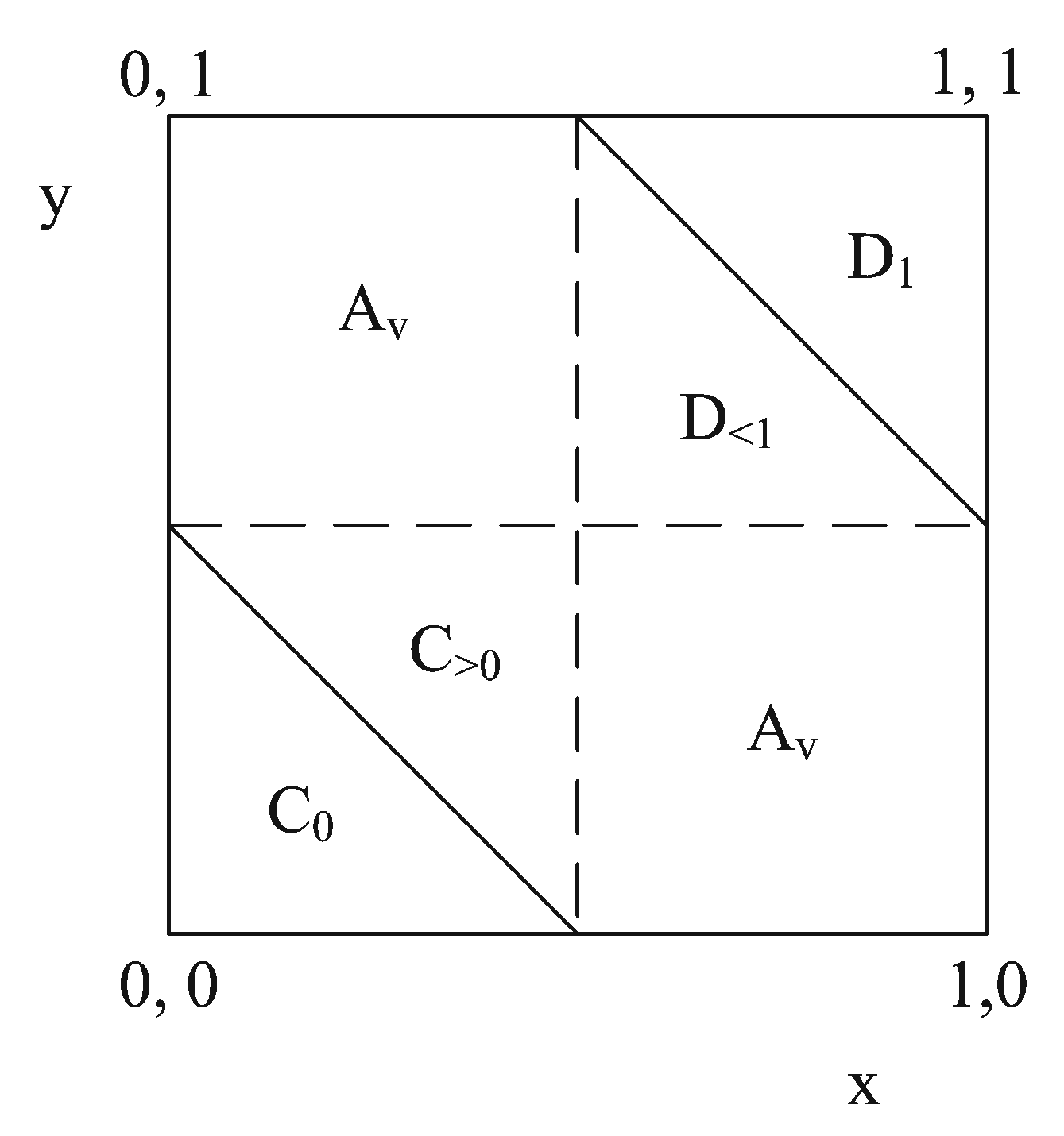
Figure 1. Classification into three classes, no, maybe, yes, by ordinal sums of conjunctive and disjunctive functions.
Make 04 00047 g001
Figure 2. Learning of the disjunctive part of classification by ordinal sums for class no.
Make 04 00047 g002
Figure 5. The original XOR data. The values on the x-axis correspond to the feature “survived”, the values on the y-axis correspond to the feature “non-survived” and the corresponding inverted values of the “target” are on the z-axis.
Make 04 00047 g005
Figure 6. The approximated XOR data with the use of p 1 = 0.076 , p 2 = 0.0731 , s = 0.012 according to Equation (14).
Make 04 00047 g006
Figure 7. Parameter estimation with the use of an evolutionary algorithm for the average case. The blue points represent the samples with r = 0.75 , whereas the red points are the ones that were created with r = 1 or r = 1.25 . The blue surface is the one created by the application of function (11) with the original r = 0.75 . The red surface is the one created by the application of the same function with the best found r = 0.88 .
Make 04 00047 g007
Figure 8. Parameter estimation with the use of an evolutionary algorithm for the conjunctive case. The blue points represent the samples with λ = 1.25 , whereas the red points are the ones that were created with λ = 0.75 or λ = 1 . The blue surface is the one created by the application of the function (10) with the original λ = 1.25 . The red surface is the one created by the application of the same function with the best found λ = 1.22 .
Make 04 00047 g008
Figure 9. State of the agent at the end of each of the 150 episodes for the averaging function. After the exploration phase, around episode 70 the agent reaches a value near 0.87 , which is similar to the solution provided by the evolutionary algorithm.
Make 04 00047 g009
Figure 10. MSE between original data and estimated solution at the end of each of the 150 episodes for the averaging function. After the exploration phase, the MSE converges to 0.
Make 04 00047 g010
Figure 11. State of the agent at the end of each of the 150 episodes for the conjunctive function. After the exploration phase, around episode 70 the agent reaches a value near 1.2 , which is similar to the solution provided by the evolutionary algorithm.
Make 04 00047 g011
Figure 12. MSE between original data and estimated solution at the end of each of the 150 episodes for the conjunctive function. After the exploration phase, the MSE converges to 0.
Make 04 00047 g012
Figure 13. The initial state of the tool for the visualisation of the experiments.
Make 04 00047 g013
Figure 14. The query window allows the user to define the quantifier function for each axis. The axis (“Axis”), quantifier mode (“Mode”) and the attributes (“Keys”) can be selected here. The bottom section shows the current selection.
Make 04 00047 g014
Figure 15. Visualisation of the Cleveland Heart Disease dataset in the classification space before adjusting λ and r.
Make 04 00047 g015
Figure 17. Result of calculating λ and r after assigning to each patient the target value of 1 for yes if the patient has heart disease and 0 for no if the patient has no heart disease. The classification space is presented as red for definitive no, green for definitive yes and a gradient from pink (tendency more to no) to turquoise (tendency more to yes) for maybe.
Make 04 00047 g017
Table 1. Data for parameter learning of the conjunctive function for the class no.
λ 1.251.251.251.250.751.251.251.251.251.25
x0.010.250.260.230.250.270.050.490.220.48
y0.410.480.390.340.350.300.490.490.060
solution00.220.1200.1200.030.4700
λ 1.251.251.250.751.251.251.251.251.251.25
x0.500.390.030.200.090.250.400.110.100.35
y0.130.390.200.300.200.090.490.500.100.07
solution0.130.2700.05000.380.1100
λ 11.251.251.251.251.251.251
x0.250.460.460.500.210.500.110.19
y0.4400.030.240.240.030.320.35
solution0.19000.2400.0300.04
Table 2. Data for parameter learning of the averaging function inclined to the class no.
r0.750.750.750.750.751.250.750.750.750.75
x0.420.370.260.100.290.290.420.320.360.35
y0.800.570.950.550.670.700.980.780.990.63
solution0.700.430.650.130.440.510.880.570.820.46
r10.750.750.750.750.751.250.750.750.75
x0.00.140.310.360.370.470.120.380.340.44
y1.00.690.960.600.920.570.590.780.570.73
solution0.50.280.730.450.760.530.230.640.400.66
r0.750.750.7510.750.750.750.750.75
x0.460.500.360.200.010.170.450.470.02
y0.560.500.740.800.630.560.710.680.98
solution0.510.500.580.500.070.210.650.640.33
Table 3. The 14 attributes of the processed Cleveland Heart Disease dataset with their specified limits. More details on the attributes in Section 6.1 and details on maximum and minimum limit in Section 6.2.
LabelMin LimitMax LimitDescription
age4065Age in years
sex01Sex
cp21Chest pain type
trestbps120140Resting blood pressure in mm Hg
chol180300Serum cholesterol in mg/dL
fbs01Fasting blood sugar
restecg02Resting electrocardiographic results
thalach160120Maximum heart rate during exercise electrocardiogram.
exang01Exercise-induced angina
oldpeak04.4ST depression relative to rest (mV)
slope13The slope of the peak exercise ST segment
(1 = upsloping, 2 = flat, 3 = downsloping)
ca03Number of major vessels coloured by fluoroscopy
thal37Thallium scintigraphic defects
(3 = normal, 6 = fixed defect, 7 = reversible defect)
num Presence of disease
Table 4. Classification outcome; one can observe that the majority of points are correctly classified. Nevertheless, since the ground truth does not provide us with the actual number of patients belonging to the maybe class, one cannot use a well-known metric as accuracy, confusion matrix or mutual information [72,73]. A human-in-the-loop approach must be used to provide the labels for the samples in the maybe class.
Patients without disease in the no section97
Patients with disease in the no section13
Patients without disease in the yes section7
Patients with disease in the yes section52
Patients without disease in the maybe section56
Patients with disease in the maybe section73
Publisher’s Note: MDPI stays neutral with regard to jurisdictional claims in published maps and institutional affiliations.