
Prospective Neural Network Model for Seismic Precursory Signal Detection in Geomagnetic Field Records


Abstract
:1. Introduction
2. Detectability of Electromagnetic Emissions from Pre-Earthquake Phenomena
3. Data and Methods

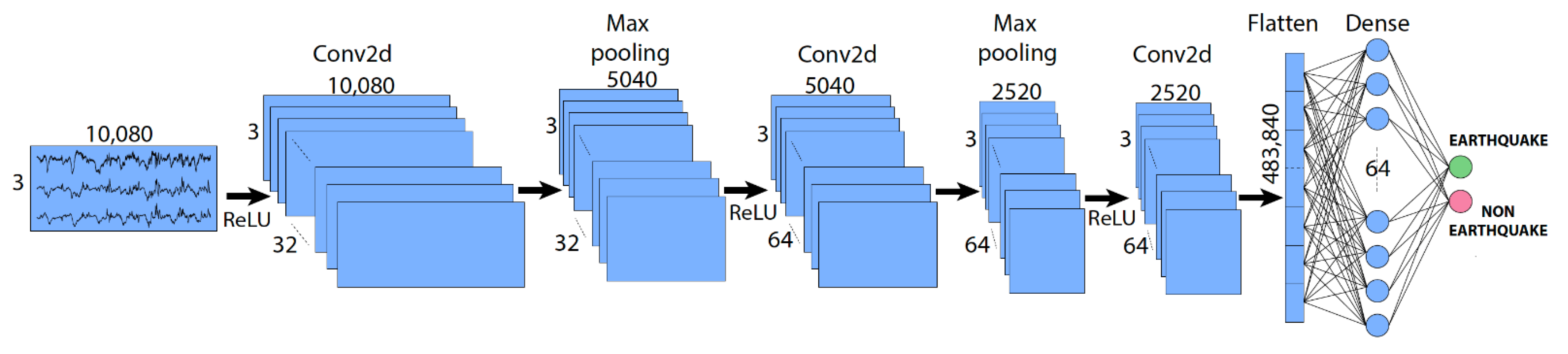
| Layer Type | No. of Output Filters | Conv. or Pooling Window Size | Padding | Activation Function | Output Shape | No. of Parameters |
|---|---|---|---|---|---|---|
| Conv2D | 32 | 3 × 3 | Yes | ReLU | (3, 10,080, 32) | 320 |
| MaxPooling | - | 1 × 2 | - | - | (3, 5040, 32) | 0 |
| Conv2D | 64 | 1 × 3 | Yes | ReLU | (3, 5040, 64) | 6208 |
| MaxPooling | - | 1 × 2 | - | - | (3, 2520, 64) | 0 |
| Conv2D | 64 | 1 × 3 | Yes | ReLU | (3, 2520, 64) | 12,352 |
| Flattened | - | - | - | - | 483,840 | 0 |
| Dense | - | - | - | Softmax | 64 | 30,965,824 |
| Dense | - | - | - | - | 2 | 130 |
4. Proof of Concept Design
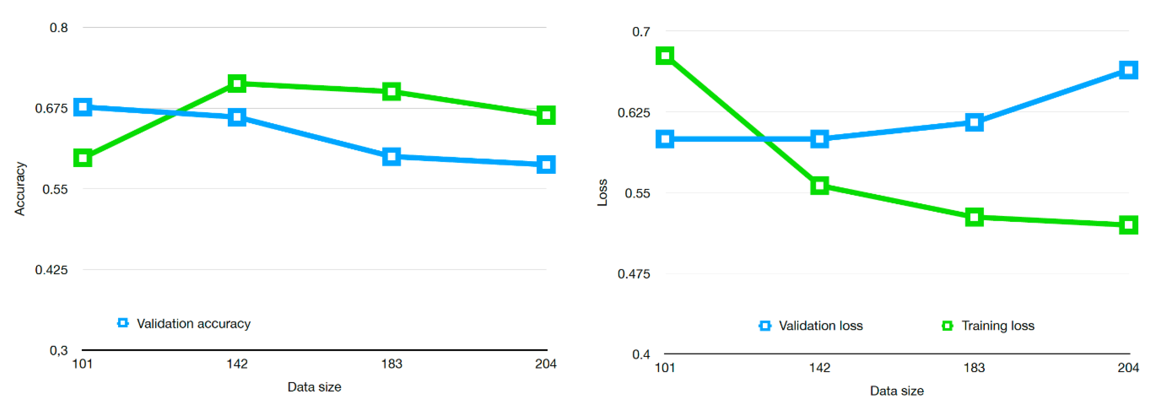
5. Preliminary Results and Future Work
- Geomagnetic field variations are not correlated with the occurrence of small-magnitude earthquakes at the predicted distances;
- An observational bias exists, implying that other geomagnetic signals obscure precursory signals and that stricter conditions need to be imposed on the detectability threshold values;
- The data available at present are insufficient to train the proposed convolutional neural network model.
6. Conclusions
Author Contributions
Funding
Institutional Review Board Statement
Informed Consent Statement
Data Availability Statement
Acknowledgments
Conflicts of Interest
References
- Shedlock, K.M.; Giardini, D.; Grunthal, G.; Zhang, P. The GSHAP global seismic hazard map. Seismol. Res. Lett. 2000, 71, 679–686. [Google Scholar] [CrossRef] [Green Version]
- Cicerone, R.D.; Ebel, J.E.; Britton, J. A systematic compilation of earthquake precursors. Tectonophysics 2009, 476, 371–396. [Google Scholar] [CrossRef]
- Currie, J.L.; Waters, C.L. On the use of geomagnetic indices and ULF waves for earthquake precursor signatures. Geophys. Res. Space Phys. 2014, 119, 992–1003. [Google Scholar] [CrossRef]
- Campbell, W.H. Introduction to Geomagnetic Fields, 2nd ed.; Cambridge University Press: Cambridge, UK, 2003. [Google Scholar]
- Stănică, D.A.; Stănică, D. Possible Correlations between the ULF Geomagnetic Signature and Mw6. 4 Coastal Earthquake, Albania, on 26 November 2019. Entropy 2021, 23, 233. [Google Scholar] [CrossRef]
- Moldovan, I.A.; Placinta, A.O.; Constantin, A.P.; Moldovan, A.S.; Ionescu, C. Correlation of geomagnetic anomalies recorded at Muntele Rosu Seismic Observatory (Romania) with earthquake occurrence and solar magnetic storms. Ann. Geophys. 2012, 55, 1. [Google Scholar]
- Xu, G.; Han, P.; Huang, Q.; Hattori, K.; Febriani, F.; Yamaguchi, H. Anomalous behaviors of geomagnetic diurnal variations prior to the 2011 off the Pacific coast of Tohoku earthquake (Mw9. 0). J. Asian Earth Sci. 2013, 77, 59–65. [Google Scholar] [CrossRef] [Green Version]
- Hayakawa, M.; Schekotov, A.; Potirakis, S.; Eftaxias, K. Criticality features in ULF magnetic field prior to the 2011 Tohoku earthquake. Proc. Jpn. Acadademy Ser. 2015, 91, 25–30. [Google Scholar] [CrossRef] [Green Version]
- Krizhevsky, A.; Sutskever, I.; Hinton, G.E. Imagenet classification with deep convolutional neural networks. Adv. Neural Inf. Process. Syst. 2012, 25, 84–90. [Google Scholar] [CrossRef] [Green Version]
- Masci, F.; Thomas, J.N. Are there new findings in the search for ULF magnetic precursors to earthquakes? J. Geophys. Res. Space Phys. 2015, 120, 10289–10304. [Google Scholar] [CrossRef] [Green Version]
- Freund, F.; Takeuchi, A.; Lau, B. Electric currents streaming out of stressed igneous rocks—A step towards understanding preearthquake low frequency EM emissions. Phys. Chem. Earth 2006, 31, 389–396. [Google Scholar] [CrossRef] [Green Version]
- Dahlgren, R.P.; Johnston, M.J.S.; Vanderbilt, V.C.; Nakaba, R.N. Comparison of the stress-stimulated current of dry and fluid-saturated gabbro samples. Bull. Seism. Soc. Am. 2014, 104, 2662–2672. [Google Scholar] [CrossRef]
- Draganov, A.B.; Inan, U.S.; Taranenko, Y.N. ULF magnetic signatures at the Earth’s surface due to ground water flow: A possible precursor to earthquakes. Geophys. Res. Lett. 1991, 18, 1127–1130. [Google Scholar] [CrossRef]
- Sasai, Y. Tectonomagnetic modeling on the basis of the linear piezomagnetic effect. Bull. Earthq. Res. Inst. Univ. Tokyo 1991, 66, 585–722. [Google Scholar]
- Eftaxias, E.; Potirakis, S.M. Current challenges for pre-earthquake electromagnetic emissions: Shed- ding light from micro-scale plastic flow, granular packings, phase transitions and self-affinity notion of fracture process. Nonlinear Processes Geophys. 2013, 20, 771–792. [Google Scholar] [CrossRef] [Green Version]
- Rabinovitch, A.; Frid, V.; Bahat, D. Surface oscillations: A possible source of fracture induced electromagnetic radiation. Tectonophysics 2007, 431, 15–21. [Google Scholar] [CrossRef]
- Koulouras, G.; Balasis, G.; Kiourktsidis, I.; Nannos, E.; Kontakos, K.; Stonham, J.; Ruzhin, Y.; Eftaxias, K.; Cavouras, D.; Nomicos, C. Discrimination between pre-seismic electromagnetic anomalies and solar activity effects. Phys. Scr. 2009, 79, 045901. [Google Scholar] [CrossRef]
- Ben-David, O.; Cohen, G.; Fineberg, J. The dynamic of the onset of frictional slip. Science 2010, 330, 211–214. [Google Scholar] [CrossRef]
- Rabinovitch, A.; Frid, V.; Bahat, D. Use of electromagnetic radiation for potential forecast of earthquakes. Geol. Mag. 2018, 155, 992–996. [Google Scholar] [CrossRef]
- Molchanov, O.A.; Hayakawa, M.; Rafalsky, V.A. Penetration characteristics of electromagnetic emissions from an underground seismic source into the atmosphere, ionosphere, and magnetosphere. J. Geophys. Res. Space Phys. 1995, 100, 1691–1712. [Google Scholar] [CrossRef]
- Gotoh, K.; Akinaga, Y.; Hayakawa, M.; Hattori, K. Principal component analysis of ULF geomagnetic data for Izu islands earthquakes in July 2000. J. Atmos. Electr. 2002, 22, 1–12. [Google Scholar] [CrossRef]
- Morgunov, V.; Malzev, S. A multiple fracture model of pre-seismic electromagnetic phenomena. Tectonophysics 2007, 431, 61–72. [Google Scholar] [CrossRef]
- Simonyan, K.; Zisserman, A. Very deep convolutional networks for large-scale image recognition. arXiv 2014, arXiv:1409.1556. [Google Scholar]
- DeVries, P.M.R.; Viégas, F.; Wattenberg, M. Deep learning of aftershock patterns following large earthquakes. Nature 2018, 560, 632–634. [Google Scholar] [CrossRef]
- Popova, I.; Rozhnoi, A.; Solovieva, M.; Levin, B.; Hayakawa, M.; Hobara, Y.; Biagi, P.F.; Schwingenschuh, K. Neural network approach to the prediction of seismic events based on low-frequency signal monitoring of the Kuril-Kamchatka and Japanese regions. Ann. Geophys. 2013, 56, 0328. [Google Scholar]
- Shahrisvand, M.; Akhoondzadeh, M.; Sharifi, M.A. Detection of gravity changes before powerful earthquakes in GRACE satellite observations. Ann. Geophys. 2014, 57, 0543. [Google Scholar] [CrossRef]
- Chollet, F. Keras. 2015. Available online: https://github.com/fchollet/keras (accessed on 1 March 2022).
- Goodfellow, I.; Bengio, Y.; Courville, A. Deep Learning (Adaptive Computation and Machine Learning Series); The MIT Press: Cambridge, MA, USA, 2017; pp. 321–359. [Google Scholar]
- Kingma, D.P.; Ba, J. Adam: A method for stochastic optimization. arXiv 2014, arXiv:1412.6980. [Google Scholar]
- Chiarabba, C.; Jovane, L.; DiStefano, R. A new view of Italian seismicity using 20 years of instrumental recordings. Tectonophysics 2005, 395, 251–268. [Google Scholar] [CrossRef]
- Şengör, A.M.C.; Tüysüz, O.; Imren, C.; Sakınç, M.; Eyidoğan, H.; Görür, N.; Le Pichon, X.; Rangin, C. The North Anatolian fault: A new look. Annu. Rev. Earth Planet. Sci. 2005, 33, 37–112. [Google Scholar] [CrossRef]
- Wenzel, F.; Lorenz, F.; Sperner, B.; Oncescu, M. Seismotectonics of the Romanian Vrancea area. In Vrancea Earthquakes: Tectonics, Hazard and Risk Mitigation; Springer: Dordrecht, The Netherlands, 1999; pp. 15–25. [Google Scholar]
- Oncescu, M.C.; Marza, V.I.; Rizescu, M.; Popa, M. The Romanian Earthquake Catalogue Between 984–1997. In Vrancea Earthquakes: Tectonics, Hazard and Risk Mitigation; Springer: Dordrecht, The Netherlands, 1999; pp. 43–47. [Google Scholar]
- Storchak, D.A.; Harris, J.; Brown, L.; Lieser, K.; Shumba, B.; Di Giacomo, D. Rebuild of the Bulletin of the International Seismological Centre (ISC)—Part 2: 1980–2010. Geosci. Lett. 2020, 7, 18. [Google Scholar] [CrossRef]
- Matzka, J.; Stolle, C.; Yamazaki, Y.; Bronkalla, O.; Morschhauser, A. The geomagnetic Kp index and derived indices of geomagnetic activity. Space Weather 2021, 19, e2020SW002641. [Google Scholar] [CrossRef]
- Yu, T.; Zhu, H. Hyper-parameter optimization: A review of algorithms and applications. arXiv 2020, arXiv:2003.05689. [Google Scholar]
- Cho, J.; Lee, K.; Shin, E.; Choy, G.; Do, S. How much data is needed to train a medical image deep learning system to achieve necessary high accuracy? arXiv 2015, arXiv:1511.06348. [Google Scholar]
- Russakovsky, O.; Deng, J.; Su, H.; Krause, J.; Satheesh, S.; Ma, S.; Huang, Z.; Karpathy, A.; Khosla, A.; Bernstein, M.; et al. ImageNet Large Scale Visual Recognition challenge. Int. J. Comput. Vis. 2015, 115, 211–252. [Google Scholar] [CrossRef] [Green Version]
- Figueroa, R.L.; Zeng-Treitler, Q.; Kandula, S.; Ngo, L.H. Predicting sample size required for classification performance. BMC Med. Inform. Decis. Mak. 2012, 12, 8. [Google Scholar] [CrossRef]
- Jaipuria, N.; Zhang, X.; Bhasin, R.; Arafa, M.; Chakravarty, P.; Shrivastava, S.; Manglani, S.; Murali, V.N. Deflating Dataset Bias using Synthetic Data Augmentation. In Proceedings of the IEEE/CVF Conference on Computer Vision and Pattern Recognition Workshops, Virtual, 14–19 June 2020; pp. 772–773. [Google Scholar]
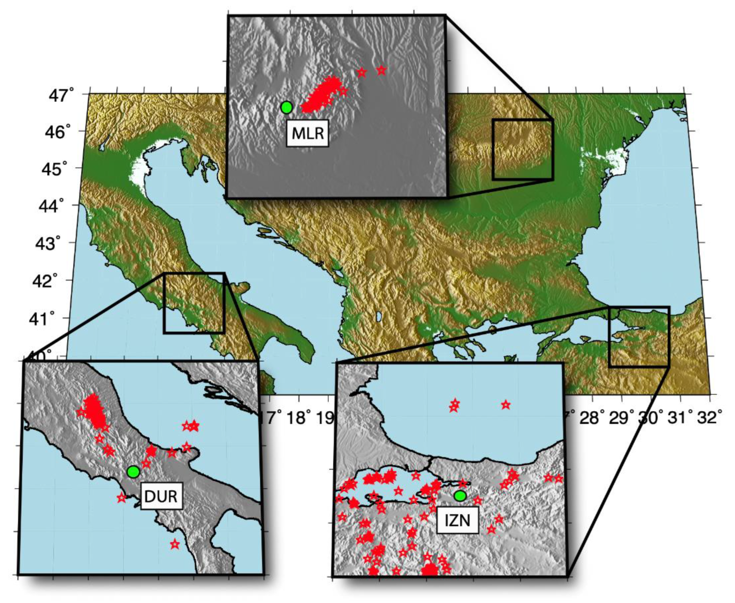


| Magnetic Observatory | Code | Country | Latitude °N | Longitude °E | Data Availability * | Data Provider | Mmax |
|---|---|---|---|---|---|---|---|
| Muntele Rosu | MLR | Romania | 45.491 | 25.945 | 2013–2022 | NIEP | 5.7 |
| Duronia | DUR | Italy | 41.390 | 14.280 | 2011–2022 | INTERMAGNET | 6.6 |
| Iznik | IZN | Türkiye | 40.500 | 29.720 | 2007–2022 | INTERMAGNET | 5.9 |
Publisher’s Note: MDPI stays neutral with regard to jurisdictional claims in published maps and institutional affiliations. |
© 2022 by the authors. Licensee MDPI, Basel, Switzerland. This article is an open access article distributed under the terms and conditions of the Creative Commons Attribution (CC BY) license (https://creativecommons.org/licenses/by/4.0/).
Share and Cite
Petrescu, L.; Moldovan, I.-A. Prospective Neural Network Model for Seismic Precursory Signal Detection in Geomagnetic Field Records. Mach. Learn. Knowl. Extr. 2022, 4, 912-923. https://doi.org/10.3390/make4040046
Petrescu L, Moldovan I-A. Prospective Neural Network Model for Seismic Precursory Signal Detection in Geomagnetic Field Records. Machine Learning and Knowledge Extraction. 2022; 4(4):912-923. https://doi.org/10.3390/make4040046
Chicago/Turabian StylePetrescu, Laura, and Iren-Adelina Moldovan. 2022. "Prospective Neural Network Model for Seismic Precursory Signal Detection in Geomagnetic Field Records" Machine Learning and Knowledge Extraction 4, no. 4: 912-923. https://doi.org/10.3390/make4040046
APA StylePetrescu, L., & Moldovan, I.-A. (2022). Prospective Neural Network Model for Seismic Precursory Signal Detection in Geomagnetic Field Records. Machine Learning and Knowledge Extraction, 4(4), 912-923. https://doi.org/10.3390/make4040046