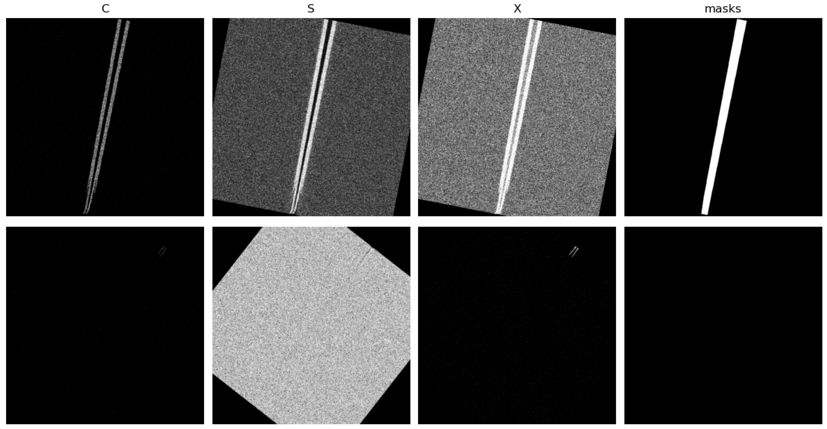
Figure 1.
Images for two wake events (one per row) are displayed in this figure. The first column on the left is the C-band images, followed by the S-band and X-band images. The final column to the right is the wake masks used for the U-Net segmentation model. Note that there is no persistent wake for the images in the second row, and therefore there is no mask. All images with a wake event have the same augmentation applied to them for consistency in the augmented dataset.
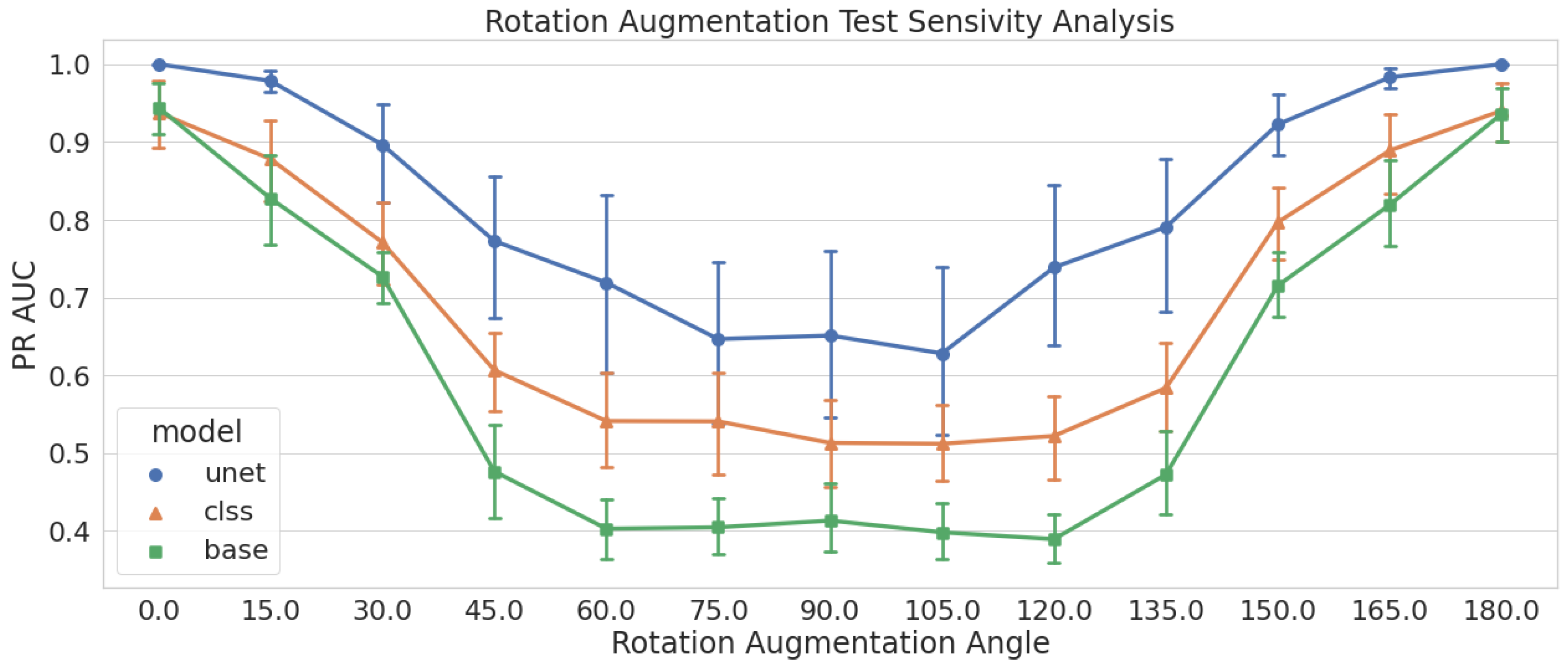
Figure 2.
Performance of models trained with no augmentations tested on all rotation augmentations sets. Models are measured using the PR AUC metric, and we see models drop to their lowest performance around the 90 rotation.
Figure 2.
Performance of models trained with no augmentations tested on all rotation augmentations sets. Models are measured using the PR AUC metric, and we see models drop to their lowest performance around the 90 rotation.
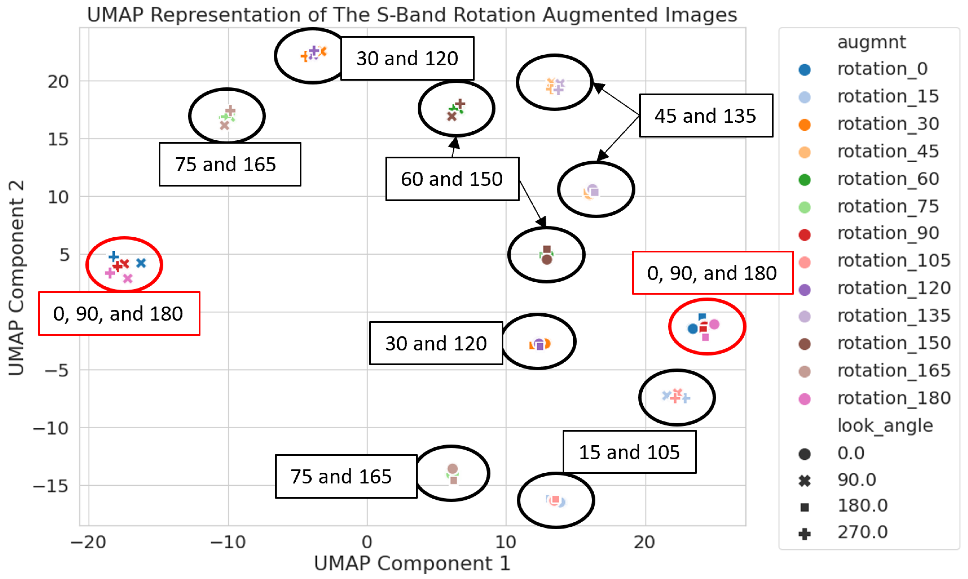
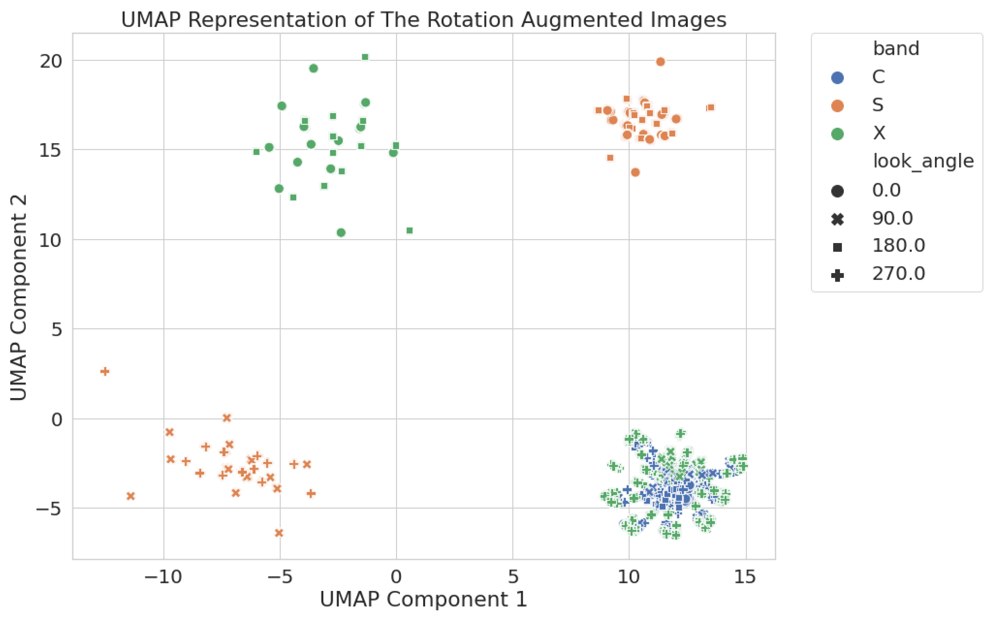
Figure 3.
S-band latent space with labels for the rotation augmentation angle of each cluster. These labels help to show that clusters are forming based on the difference of the rotation angle from 0° or 90°, revealing inadvertent clustering based on the rotation of a square image.
Figure 3.
S-band latent space with labels for the rotation augmentation angle of each cluster. These labels help to show that clusters are forming based on the difference of the rotation angle from 0° or 90°, revealing inadvertent clustering based on the rotation of a square image.
Figure 4.
Circular cropping is applied to the images so that rotation augmentations do not create triangular clippings that are seen in
Figure 1. Any time a rotation is applied to these images, there is no change in the amount or shape of overall information in the image—only the orientation of the wake. Note that there is no persistent wake for the images in the second row, and therefore there is no mask.
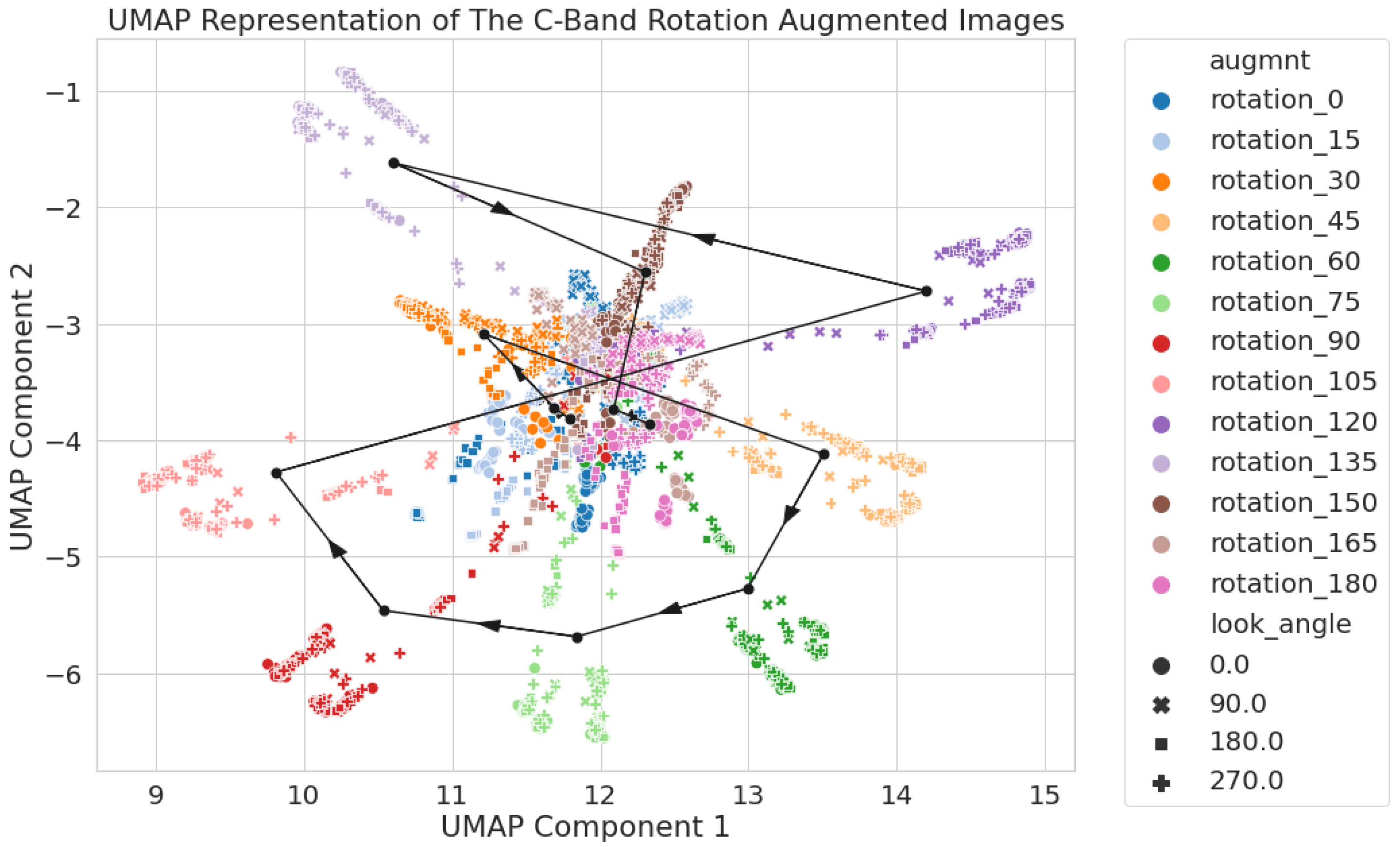
Figure 5.
C-band only 2D UMAP latent space using circular crop images. Each augmentation set has its mean location pin-pointed with a black dot and connected via a black line with arrows to show the direction of the increasing rotation angle.
Figure 5.
C-band only 2D UMAP latent space using circular crop images. Each augmentation set has its mean location pin-pointed with a black dot and connected via a black line with arrows to show the direction of the increasing rotation angle.
Figure 6.
S-band only 2D UMAP latent space using circular crop images. All rotation augmentations are used, and the results show two clusters of images based on the look angle, 0 and 180 in the upper right and 90 and 270 are in the lower left.
Figure 6.
S-band only 2D UMAP latent space using circular crop images. All rotation augmentations are used, and the results show two clusters of images based on the look angle, 0 and 180 in the upper right and 90 and 270 are in the lower left.
Figure 7.
X-band only 2D UMAP latent space using circular crop images. All rotation augmentations are used, and the results show two clusters of images based on the look angle, 0
and 180
in the upper left and 90
and 270
are in the lower right. The 90
and 270
look angle images form a pattern similar to C-band (
Figure 5), while the 90
and 270
look angle images form a pattern similar to S-band (
Figure 6).
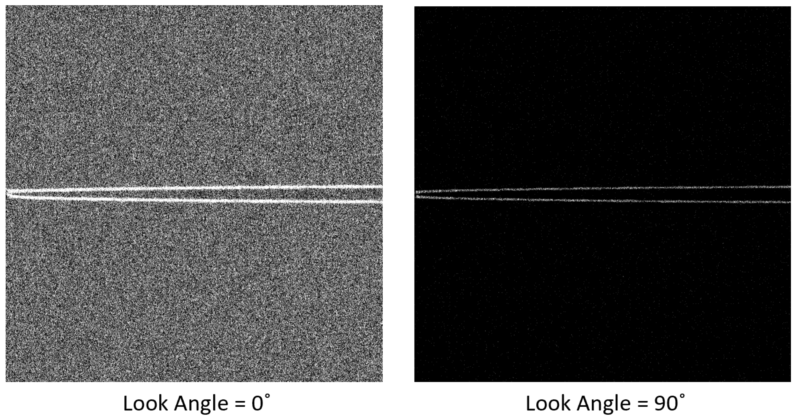
Figure 8.
Comparison of the same wake event in the X-Band. On the left is the wake with a look angle of 0°, and on the right is the wake with a look angle of 90°. All other generation parameters are the same for these images. The noise level in the background ocean surface in the left is typical of 0° and 180° look angles, while the one on the right is typical of look angles of 90° and 270°.
Figure 9.
Two-dimensional UMAP latent space generated using all rotation-augmented circular crop images. C-band and the 90 and 270 look angle X-band images cluster together in the lower right of the image. S-band and the 0 and 180 X-band images all cluster apart.
Figure 9.
Two-dimensional UMAP latent space generated using all rotation-augmented circular crop images. C-band and the 90 and 270 look angle X-band images cluster together in the lower right of the image. S-band and the 0 and 180 X-band images all cluster apart.
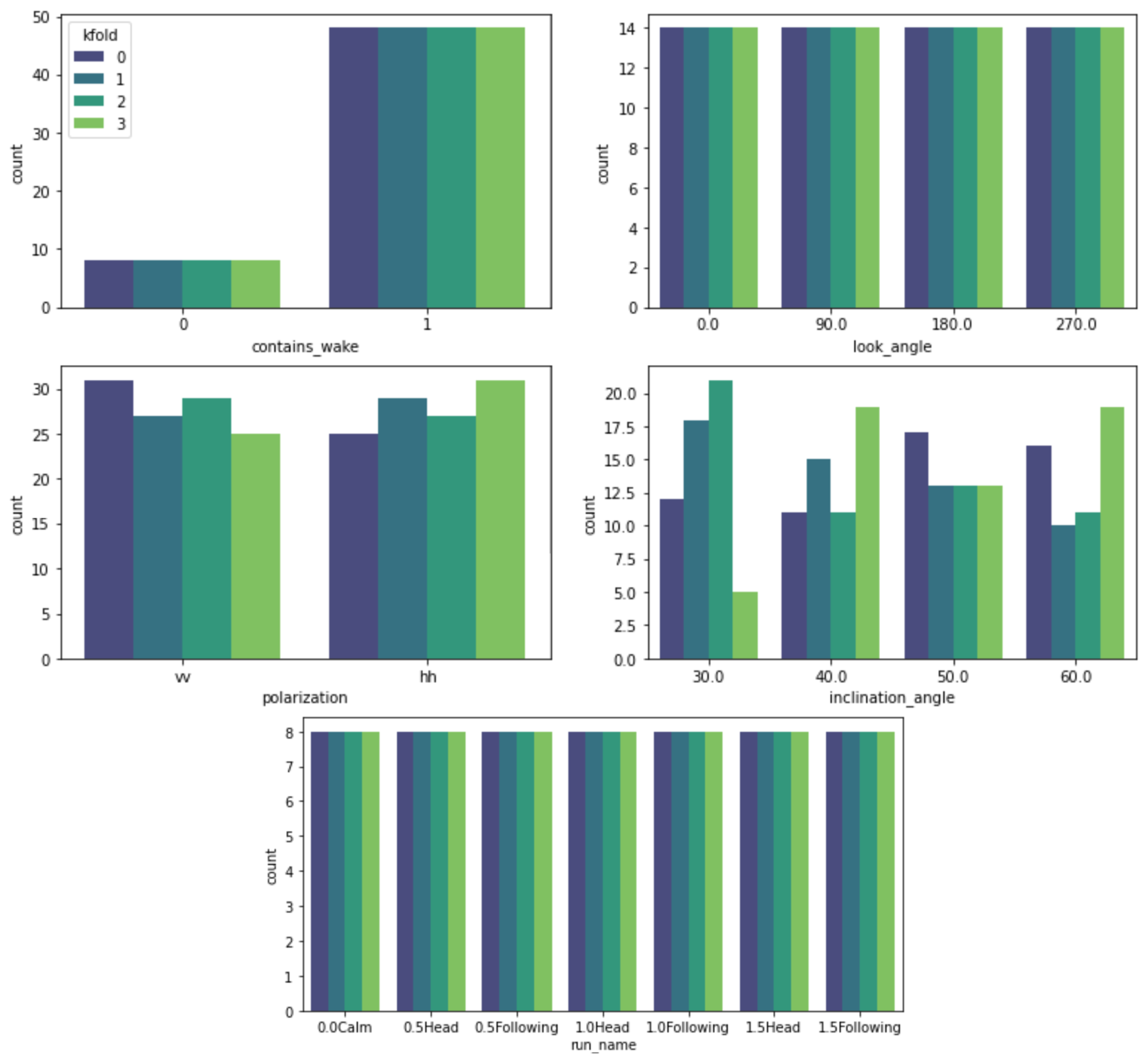
Figure 10.
Distribution of the metadata features for the four training and testing folds used in the baseline study. The folds are designed to stratify contains_wake, look_angle, and run_name to have matching distributions for each fold.
Figure 10.
Distribution of the metadata features for the four training and testing folds used in the baseline study. The folds are designed to stratify contains_wake, look_angle, and run_name to have matching distributions for each fold.
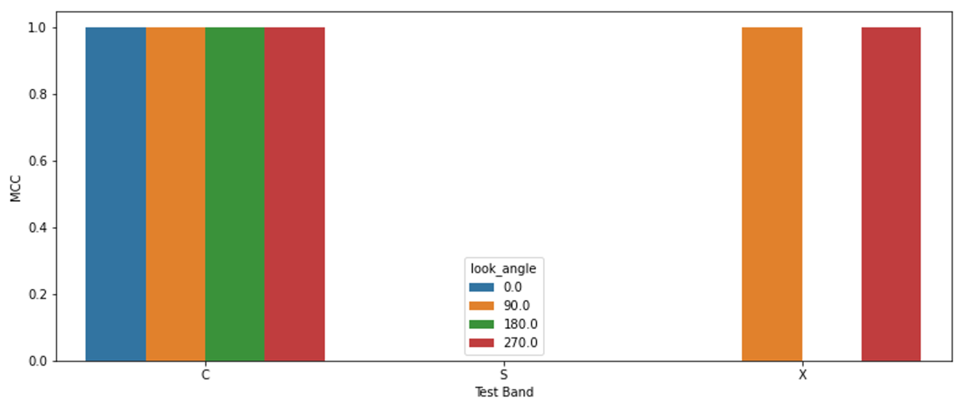
Figure 11.
Results for the baseline latent space study. This study is run with four sets of the data using a combination of non-rotated or randomly-rotated images and either normal crop image or circular crop images. All sets have matching results, so only one set is presented. The models trained on C-band performed perfectly for C-band and the 90 and 270 look angle X-band images, while it did poorly for S-band and the 0 and 180 look angle X-band images. These results confirm the latent space representation of the data has a relation to the model’s performance on that data. The results also convey that latent space is useful regardless of image cropping or applied augmentations. However, cropping and augmentations are consistent between the training and testing images—the only difference is the SAR band.
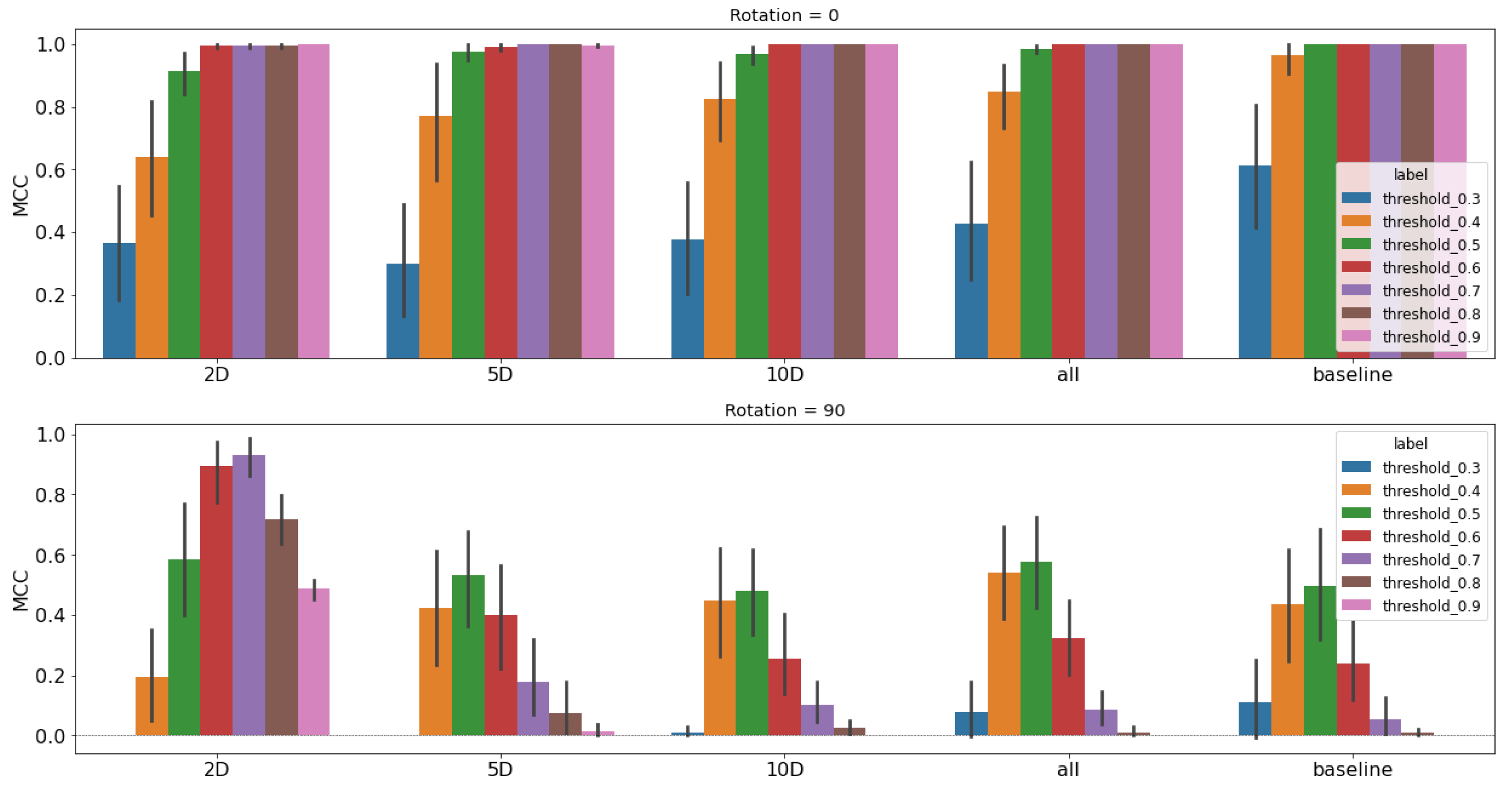
Figure 12.
Performance study results for C-band using the unet classifier architecture. Each model is trained with an even split of augmented and non-augmented images, then tested on 0 rotated images (top row) and 90 rotated images (bottom row). We use the MCC metric and a sweep of thresholds to present a profile of performance rather than single metric. Training augmentations are chosen from different latent space representations; moving left to right, they are 2D, 5D, 10D, a combined selection using all three, and then finally the baseline performance is on the far right for comparison.
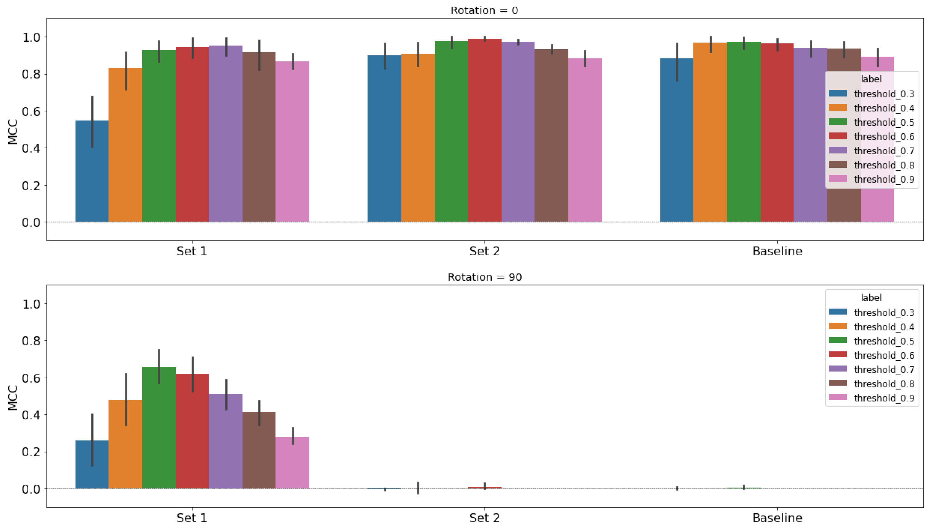
Figure 13.
Performance study results for S-band using the unet classifier architecture. Each model is trained with an even split of augmented and non-augmented images, then tested on 0 rotated images (top row) and 90 rotated images (bottom row). We use the MCC metric and a sweep of thresholds to present a profile of performance rather than single metric. Training augmentations are chosen from the 2D latent space representations. Set 1 chooses based on the 90/270 look angle images, and Set 2 chooses based on the 0/180 look angle images. The baseline model performance is on the far right for comparison.
Figure 14.
Performance study results for X-band using the unet classifier architecture. Each model is trained with an even split of augmented and non-augmented images, then tested on 0 rotated images (top row) and 90 rotated images (bottom row). We use the MCC metric and a sweep of thresholds to present a profile of performance rather than single metric. Training augmentations are chosen from the 2D latent space representations. Set 1 chooses based on the 90/270 look angle images, and Set 2 chooses based on the 0/180 look angle images. The baseline model performance is on the far right for comparison.
Table 1.
Run matrix for SAR image generation from [
17]. The look angle is the azimuth angle between the radar direction and the ship direction, and the inclination angle is the angle between the vertical axis and the direction from the radar to the ship wake [
18].
Table 1.
Run matrix for SAR image generation from [
17]. The look angle is the azimuth angle between the radar direction and the ship direction, and the inclination angle is the angle between the vertical axis and the direction from the radar to the ship wake [
18].
| Parameter | Possible Values |
|---|
| SAR band | C, S, X |
| Look angle | 0, 90, 180, 270 |
| Polarization | VV, HH |
| Inclination angle | 30, 40, 50, 60 |
Table 2.
Mean 2D UMAP coordinates for the C-band circular crop images from the 2D latent space representation, as shown in
Figure 9. For each augmentation set, the rotation angle and coordinates are listed.
Table 2.
Mean 2D UMAP coordinates for the C-band circular crop images from the 2D latent space representation, as shown in
Figure 9. For each augmentation set, the rotation angle and coordinates are listed.
| Rotation Angle | Mean UMAP Component 1 | Mean UMAP Component 2 |
|---|
| 0 | 11.79 | −3.82 |
| 15 | 11.69 | −3.72 |
| 30 | 11.21 | −3.09 |
| 45 | 13.51 | −4.12 |
| 60 | 12.99 | −5.27 |
| 75 | 11.84 | −5.68 |
| 90 | 10.54 | −5.46 |
| 105 | 9.81 | −4.27 |
| 120 | 14.20 | −2.72 |
| 135 | 10.61 | −1.62 |
| 150 | 12.30 | −2.56 |
| 165 | 12.09 | −3.73 |
| 180 | 12.33 | −3.86 |
Table 3.
Mahalanobis distances between the 90
rotated image set and every other rotated augmentation set in the C-band latent space. Two-dimensional distances are calculated using the coordinates in
Table 2, and a similar procedure is used for 5D and 10D representations. The All dimension sums the distances from 2D, 5D, and 10D. The far right column lists the closest rotation angle (
) to 90
.
| Dim. | 0 | 15 | 30 | 45 | 60 | 75 | 90 | 105 | 120 | 135 | 150 | 165 | 180 | |
|---|
| 2D | 1.72 | 1.75 | 2.10 | 2.69 | 2.06 | 1.12 | - | 1.22 | 3.78 | 3.32 | 2.85 | 1.93 | 1.99 | 75 |
| 5D | 2.83 | 2.52 | 4.24 | 3.12 | 3.89 | 4.41 | - | 4.55 | 3.65 | 3.39 | 4.07 | 2.71 | 2.72 | 15 |
| 10D | 3.53 | 4.31 | 4.92 | 4.99 | 4.99 | 4.99 | - | 5.00 | 5.00 | 5.00 | 5.00 | 4.48 | 4.94 | 0 |
| All | 8.09 | 8.58 | 11.27 | 10.80 | 10.94 | 10.51 | - | 10.76 | 12.43 | 11.70 | 11.91 | 9.13 | 9.65 | 0 |
Table 4.
Training augmentation sets chosen using different latent space representations (UMAP Dimension) for the C-band study. Training augmentations are selected based on the smallest Mahalanobis distance between the 90 rotated images and every other augmentation set. The All UMAP Dimension uses a combination of distances from the 2D, 5D, and 10D latent spaces.
| Band | UMAP Dimensions | Train Augmentations | Test Augmentations |
|---|
| C | 2D | 0, 75 | 0, 90 |
| C | 5D | 0, 15 | 0, 90 |
| C | 10D | 0, 15 | 0, 90 |
| C | All | 0, 15 | 0, 90 |
Table 5.
C-band results tabulating unet model training data, testing data, the peak MCC performance with 95% confidence interval (CI), and the corresponding threshold.
Table 5.
C-band results tabulating unet model training data, testing data, the peak MCC performance with 95% confidence interval (CI), and the corresponding threshold.
| Dimensions | Training Rotation | Testing Rotation | MCC | 95% CI | Threshold |
|---|
| 2 | 0, 75 | 0 | 1.0 | N/A | 0.9 |
| 5 | 0, 15 | 0 | 1.0 | N/A | 0.7 |
| 10 | 0, 15 | 0 | 1.0 | N/A | 0.6 |
| All | 0, 15 | 0 | 1.0 | N/A | 0.6 |
| Baseline | 0 | 0 | 1.0 | N/A | 0.5 |
| 2 | 0, 75 | 90 | 0.93 | 0.069 | 0.7 |
| 5 | 0, 15 | 90 | 0.53 | 0.17 | 0.5 |
| 10 | 0, 15 | 90 | 0.48 | 0.16 | 0.5 |
| All | 0, 15 | 90 | 0.58 | 0.17 | 0.5 |
| Baseline | 0 | 90 | 0.49 | 0.19 | 0.5 |
Table 6.
Training augmentation sets chosen using different look angles (0 and 75 for Set 1, and 0 and 180 for Set 2) for the S- and X-band studies. Training augmentations are selected based on the smallest Mahalanobis distance between the 90 rotated images and every other augmentation set.
Table 6.
Training augmentation sets chosen using different look angles (0 and 75 for Set 1, and 0 and 180 for Set 2) for the S- and X-band studies. Training augmentations are selected based on the smallest Mahalanobis distance between the 90 rotated images and every other augmentation set.
| Band | Set | UMAP Dimensions | Train Augmentations | Test Augmentations | Look Angle |
|---|
| S | 1 | 2D | 0, 75 | 0, 90 | 90/270 |
| S | 2 | 2D | 0, 180 | 0, 90 | 0/180 |
| X | 1 | 2D | 0, 75 | 0, 90 | 90/270 |
| X | 2 | 2D | 0, 180 | 0, 90 | 0/180 |
Table 7.
S-band results tabulating unet model training data, testing data, the peak MCC performance with 95% confidence interval (CI), and the corresponding threshold.
Table 7.
S-band results tabulating unet model training data, testing data, the peak MCC performance with 95% confidence interval (CI), and the corresponding threshold.
| Set | Training Rotation | Testing Rotation | MCC | 95% CI | Threshold |
|---|
| 1 | 0, 75 | 0 | 0.95 | 0.054 | 0.7 |
| 2 | 0, 180 | 0 | 0.99 | 0.011 | 0.6 |
| Baseline | 0 | 0 | 0.97 | 0.056 | 0.4 |
| 1 | 0, 75 | 90 | 0.66 | 0.092 | 0.5 |
| 2 | 0, 180 | 90 | 0.010 | 0.021 | 0.6 |
| Baseline | 0 | 90 | 0.0057 | 0.012 | 0.5 |
Table 8.
X-band results tabulating unet model training data, testing data, the peak MCC performance with 95% confidence interval (CI), and the corresponding threshold.
Table 8.
X-band results tabulating unet model training data, testing data, the peak MCC performance with 95% confidence interval (CI), and the corresponding threshold.
| Set | Training Rotation | Testing Rotation | MCC | 95% CI | Threshold |
|---|
| 1 | 0, 75 | 0 | 1.0 | N/A | 0.8 |
| 2 | 0, 180 | 0 | 1.0 | N/A | 0.4 |
| Baseline | 0 | 0 | 1.0 | N/A | 0.5 |
| 1 | 0, 75 | 90 | 0.82 | 0.11 | 0.5 |
| 2 | 0, 180 | 90 | 0.048 | 0.071 | 0.3 |
| Baseline | 0 | 90 | 0.093 | 0.13 | 0.3 |


