A Comparison of Surrogate Modeling Techniques for Global Sensitivity Analysis in Hybrid Simulation

Abstract

Hybrid simulation is a method used to investigate the dynamic response of a system subjected to a realistic loading scenario. The system under consideration is divided into multiple individual substructures, out of which one or more are tested physically, whereas the remaining are simulated numerically. The coupling of all substructures forms the so-called hybrid model. Although hybrid simulation is extensively used across various engineering disciplines, it is often the case that the hybrid model and related excitation are conceived as being deterministic. However, associated uncertainties are present, whilst simulation deviation, due to their presence, could be significant. In this regard, global sensitivity analysis based on Sobol’ indices can be used to determine the sensitivity of the hybrid model response due to the presence of the associated uncertainties. Nonetheless, estimation of the Sobol’ sensitivity indices requires an unaffordable amount of hybrid simulation evaluations. Therefore, surrogate modeling techniques using machine learning data-driven regression are utilized to alleviate this burden. This study extends the current global sensitivity analysis practices in hybrid simulation by employing various different surrogate modeling methodologies as well as providing comparative results. In particular, polynomial chaos expansion, Kriging and polynomial chaos Kriging are used. A case study encompassing a virtual hybrid model is employed, and hybrid model response quantities of interest are selected. Their respective surrogates are developed, using all three aforementioned techniques. The Sobol’ indices obtained utilizing each examined surrogate are compared with each other, and the results highlight potential deviations when different surrogates are used.

1. Introduction

Hybrid simulation (HS), also known as hardware-in-the-loop (HiL), is a method used to investigate the dynamic response of a system subjected to a realistic loading scenario. The system under consideration is divided into multiple individual substructures, out of which one or more are tested physically and, thus, correspond to the physical substructures (PS), whereas the remaining substructures are simulated numerically, namely, the numerical substructures (NS). The coupling of PS and NS forms the so-called hybrid model. The response of the latter is obtained from a step-by-step numerical solution of the equations governing the motion of the underlying hybrid model, combined with measurements acquired from the PS. Therefore, the calculation of the next HS time step is computed online. An arrangement of transfer systems, e.g., servo-controlled motors or actuators, is used to deliver the motion between NS and PS. The employed transfer system accounts for the substructure coupling and, hence, for synchronizing their dynamic boundary conditions in every time step of the HS. From the coupling of substructures, several challenges arise, e.g., time delays due to inherent transfer system dynamics or due to computational power needed to compute the NS response. Advanced control techniques [1,2,3,4] and model order reduction methods [5,6] have been used to tackle such issues. Albeit the challenges, the HS approach is beneficial since it can be used to experimentally study the inner workings of specific substructures over their linear regime and, hence, acquire realistic results but without constructing the entire considered system nor risking damaging it. A detailed overview of HS can be found in [7,8].

HS is widely used across different engineering disciplines [9,10,11,12,13,14,15]. However, it is often the case that the hybrid model and related excitation are conceived as being deterministic. Nonetheless, this assumption does not reflect real-world structures and systems, as loading is stochastic, whereas hybrid model parameters may be highly uncertain. A thorough investigation of all possible parameter and excitation variations is not feasible considering the cost related to an individual HS evaluation. Still, uncertainties are present whilst simulation deviation, due to their presence, could be significant.

In this regard, surrogate modeling is proposed to perform global sensitivity analysis (GSA) of a quantity of interest (QoI) hybrid model response with respect to a set of input parameters originating from both substructures and excitation [16,17]. GSA aims to quantitatively determine the degree each input parameter affects the selected QoI of the hybrid model response. Sobol’ indices are a popular methodology to perform variance-based GSA in which the variance of the response QoI is decomposed as a sum of contributions related to each input variable or combination with each other [18]. Monte Carlo simulations can be used to estimate Sobol’ indices. Nonetheless, for each index estimation, $\mathcal{O}\left({10}^3\right)$ model evaluations would be required [16]. To alleviate this burden, surrogate models of the QoI response can be developed. Surrogates (i.e., metamodels) are used to substitute an expensive-to-compute model with an inexpensive-to-compute surrogate, and are developed using machine learning data-driven regression techniques. Therefore, Monte Carlo simulations using the developed surrogates can be performed at affordable cost, and Sobol’ indices’ estimation becomes easier to compute. In particular, for the case that a polynomial chaos expansion (PCE) is constructed, then the Sobol’ indices can be computed analytically as a byproduct of the polynomial coefficients at no additional cost [19,20].

As explained in [16], PCE is used to surrogate the hybrid model response and to then compute the Sobol’ indices. This study extends the GSA framework proposed in [16] by utilizing multiple and different surrogate modeling techniques to conduct GSA via Sobol’ indices in HS. In particular, apart from PCE, Kriging (i.e., Gaussian process) and polynomial chaos Kriging (PCK) are used to surrogate the selected hybrid model QoI responses and to perform GSA. In addition, this study serves also as a demonstration of how the obtained Sobol’ indices could possibly deviate from each other when different surrogate modeling techniques are used. To validate the performance of the aforementioned methodologies, a case study encompassing a virtual hybrid model is employed, and specific QoI of the hybrid model response are selected. Surrogates for the selected QoI are constructed, and their performance is evaluated. Sobol’ indices are computed using each developed surrogate, and a comparison with each other is made to highlight potential deviations. The results demonstrate the effectiveness of each examined surrogate modeling method to perform GSA in HS. It should be noted that the utilized methodologies for conducting GSA handle the hybrid model as a black-box, and thus, they can be applied to any dynamic system investigated via HS.

This paper is organized as follows. Section 2 and Section 3 present the background of the examined surrogate modeling methods as well as the GSA with Sobol’ indices. Section 4 presents the case study with the virtual hybrid model and Section 5 discusses the respective results. Finally, Section 6 presents the overall conclusions of this study.

2. Surrogate Modeling Methods

Considering an input vector $\mathit{X}\in {\mathcal{D}}_{\mathit{X}}\subset {\mathbb{R}}^N$ and a computational model $\mathit{Y}=\mathcal{M}\left(\mathit{X}\right)$ with $\mathit{Y}\in {\mathbb{R}}^N$, machine learning data-driven regression algorithms formulate a map ${\mathcal{M}}^s:\mathit{X}\mapsto \mathit{Y}$ based on an obtained sample set of input points $\mathit{X}={\left\{{\mathit{x}}^{\left(1\right)},\dots ,{\mathit{x}}^{\left(N\right)}\right\}}^T$ and of the respective output values, i.e., model evaluations or experimental measurements, $\mathit{Y}={\left\{{\mathit{y}}^{\left(1\right)},\dots ,{\mathit{y}}^{\left(N\right)}\right\}}^T$. The set of $\mathit{X},\mathit{Y}$ realizations corresponds to the so-called experimental design (ED).

2.1. Polynomial Chaos Expansion

PCE is a well-known uncertainty quantification spectral method used to substitute the dynamics of an expensive-to-compute numerical model with an inexpensive-to-compute surrogate (i.e., metamodel), representing the outputs of the model by a polynomial function of its inputs [21,22]. It is proven to be a powerful surrogate technique used in a wide variety of engineering contexts to replicate the dynamic response of complex high-dimensional models [16,23,24].

In more detail, given a random input vector $\mathit{X}$ with independent components expressed by the joint PDF $f_{\mathit{X}}$ and a finite variance computational model $Y=\mathcal{M}\left(\mathit{X}\right)$, such that $\mathbb{E}\left[Y^2\right]={\int }_{{\mathcal{D}}_{\mathit{X}}}{\mathcal{M}}^2\left(\mathit{x}\right)f_{\mathit{X}}\left(\mathit{x}\right)d\mathit{x}<\infty$, the PCE of $\mathcal{M}\left(\mathit{X}\right)$ follows:

$$Y=\mathcal{M}\left(\mathit{X}\right)\approx {\mathcal{M}}^{PCE}\left(\mathit{X}\right)=\sum _{\alpha \in {\mathbb{N}}^N}{y}_{\mathbf{\alpha }}{\Psi }_{\mathbf{\alpha }}\left(\mathit{X}\right).$$

(1)

The PCE function is built on the ${\Psi }_{\mathbf{\alpha }}\left(\mathit{X}\right)$ multivariate orthonormal polynomial basis with respect to the input vector $f_{\mathit{X}}$. The degree of the ${\Psi }_{\mathbf{\alpha }}$ polynomials components is identified by the $\mathbf{\alpha }=({\alpha }_1,\cdots ,{\alpha }_N),\alpha \in {\mathbb{N}}^N$ multi-index for each of the input variables, while $y_{\alpha }$ corresponds to the polynomial coefficients.

2.1.1. Polynomial Basis

The multivariate polynomials are constructed as a tensor product of their univariate orthonormal polynomials ${\varphi }_k^{\left(i\right)}\left(x^{\left(i\right)}\right)$, such that

$${\Psi }_{\mathbf{\alpha }}\left(\mathit{X}\right)=\prod _{i=1}^N{\varphi }_{{\alpha }_i}^{\left(i\right)}\left(x^{\left(i\right)}\right).$$

(2)

The latter meets the orthonormality criteria:

$$〈{\varphi }_j^{\left(i\right)}(x^{\left(i\right)}),{\varphi }_k^{\left(i\right)}(x^{\left(i\right)})〉={\int }_{{\mathcal{D}}_{X_i}}{\varphi }_j^{\left(i\right)}(x^{\left(i\right)}){\varphi }_k^{\left(i\right)}(x^{\left(i\right)})f_{X_i}(x^{\left(i\right)})d{x}_i={\delta }_{jk},$$

(3)

where i corresponds to the input variable, j and k to the polynomial degree, $f_{X_i}\left(x^{\left(i\right)}\right)$ to the $i$-input marginal PDF and ${\delta }_{jk}$ to the Kronecker symbol. The selection of the univariate orthonormal polynomial families depends on the marginal PDF of each input variable to which they are orthogonal, e.g., if an input variable follows the uniform/Gaussian distribution, then the Legendre/Hermite orthogonal polynomial family is used respectively for this specific input variable [22,25].

2.1.2. Truncation Schemes

Once the univariate polynomials families are selected for each input variable, the next step is the construction of the PCE following Equation (1). However, because the sum of Equation (1) consists of infinite terms, it is often truncated to a finite number of terms for practical reasons. Hence, the truncated basis is defined as $\mathcal{A}\subset {\mathbb{N}}^N$, and the PCE of $\mathcal{M}\left(\mathit{X}\right)$ admits

$${\mathcal{M}}^{PCE}\left(\mathit{X}\right)=\sum _{\mathbf{\alpha }\in \mathcal{A}}{y}_{\mathbf{\alpha }}{\Psi }_{\mathbf{\alpha }}\left(\mathit{X}\right).$$

(4)

The performance of PCE is closely connected with the truncation scheme used. Underfitting or overfitting is possible when too many terms are discarded or introduced, respectively [24]. In the standard basis truncation scheme [22] the maximum degree $p\in {\mathbb{N}}^{+}$ is defined such that the degree of each polynomial is capped by this value. Therefore, the standard basis truncation scheme consists of $\left(\genfrac{}{}{0pt}{}{N+p}{p}\right)=\frac{(N+p)!}{N!p!}$ elements and follows

$${\mathcal{A}}^{N,p}=\left\{\mathbf{\alpha }\in {\mathbb{N}}^N:|\mathbf{\alpha }|\le p\right\},$$

(5)

where N corresponds to the number of input variables of $\mathcal{M}\left(\mathit{X}\right)$ and $|\mathbf{\alpha }|={\sum }_{i=1}^N{\alpha }_i$ to the total degree of all polynomials in $\Psi$. To further reduce the polynomial basis size, additional truncation schemes were developed, namely, the maximum interaction and hyperbolic truncation scheme.

In the maximum interaction truncation scheme [25], the basis of Equation (5) is reduced such that the $\mathbf{\alpha }$ indices to include at most are r non-zero components, and thus the rank of $\mathbf{\alpha }$ is decreased [25]. Accordingly, Equation (5) is written as

$${\mathcal{A}}^{N,p,r}=\left\{\mathbf{\alpha }\in {\mathcal{A}}^{N,p}:{\left||\mathbf{\alpha }|\right|}_0\le r\right\},$$

(6)

where ${\left||\mathbf{\alpha }|\right|}_0={\sum }_{i=1}^N{\mathbb{1}}_{\{{\alpha }_i>0\}}$ and ${\mathbb{1}}_{\{{\alpha }_i>0\}}$ is the indicator function.

The hyperbolic (i.e., q-norm) truncation scheme [26] reforms the basis of Equation (5) such that

$${\mathcal{A}}^{N,p,q}=\left\{\mathbf{\alpha }\in {\mathcal{A}}^{N,p}:{\left||\mathbf{\alpha }|\right|}_q\le p\right\},$$

(7)

where ${\left||\mathbf{\alpha }|\right|}_q={\left({\sum }_{i=1}^N{a}_i^q\right)}^{\frac{1}{q}}$ and $q\in (0,1]$.

2.1.3. PCE Coefficient Calculation

Once the truncation scheme is determined, the next step is the calculation of coefficients $\mathit{y}=\{{\mathit{y}}_{\mathbf{\alpha }},\mathbf{\alpha }\in \mathcal{A}\}$ of Equation (4). Various methods were developed to do this [25]. One of these techniques is the least-squares minimization [27]. This is an non-intrusive method, meaning that the coefficients are obtained after post-processing the ED points. More specifically, Equation (4) is reformed as

$${\mathcal{M}}^{PCE}\left(\mathit{X}\right)=\sum _{j=0}^{P-1}{y}_j{\Psi }_j\left(\mathit{X}\right)+{\epsilon }_P={\mathit{y}}^T\mathsf{\Psi }\left(\mathit{X}\right)+{\epsilon }_P,$$

(8)

where $\mathit{y}={(y_0,\cdots ,y_{P-1})}^T$ denote the PCE coefficients, ${\epsilon }_P$ the truncation error, $\mathsf{\Psi }\left(\mathit{X}\right)={\{{\Psi }_0\left(\mathit{X}\right),\cdots ,{\Psi }_{P-1}\left(\mathit{X}\right)\}}^T$ the multivariate orthonormal polynomials, and $P=\left(\genfrac{}{}{0pt}{}{N+p}{p}\right)$. Then, the PCE coefficients are obtained by solving

$$\widehat{\mathit{y}}=arg\underset{\mathit{y}\in {\mathbb{R}}^{\left|\mathcal{A}\right|}}{min}\mathbb{E}\left[{\left({\mathit{y}}^T\mathsf{\Psi }\left(\mathit{X}\right)-\mathcal{M}\left(\mathit{X}\right)\right)}^2\right].$$

(9)

The solution of Equation (9) is attained by ordinary least-squares (OLS) and follows:

$$\widehat{\mathit{y}}={\left({\mathit{A}}^T\mathit{A}\right)}^{-1}{\mathit{A}}^T\mathit{Y},$$

(10)

where the experimental matrix is $A_{ij}={\Psi }_j\left({\mathit{x}}^{\left(i\right)}\right)$ with $i=1,\cdots ,N$ and $j=0,\cdots ,P-1$.

However, for $N<P-1$, the ${\mathit{A}}^T\mathit{A}$ matrix is non-invertible, and thus the OLS problem cannot be solved [24,28]. Nonetheless, through sparse regression, accurate surrogates can be constructed with fewer coefficients. A way to achieve sparse regression in high-dimensions is by a modification of the least-squares minimization method. In more detail, a penalty term is introduced in Equation (9) and the latter is modified as

$$\widehat{\mathit{y}}=arg\underset{\mathit{y}\in {\mathbb{R}}^{\left|\mathcal{A}\right|}}{min}\mathbb{E}\left[{\left({\mathit{y}}^T\Psi \left(\mathit{X}\right)-\mathcal{M}\left(\mathit{X}\right)\right)}^2\right]+\lambda {\left|\left|\mathit{y}\right|\right|}_1,$$

(11)

where ${\left|\left|\mathit{y}\right|\right|}_1={\sum }_{\mathbf{\alpha }\in \mathcal{A}}\left|y_{\mathbf{\alpha }}\right|$ and $\lambda$ is a parameter of the penalty term. This penalty term causes the minimization to facilitate sparse solutions. One of the widely utilized techniques, used to solve the minimization problem of Equation (11), is the least angle regression (LAR) algorithm [26]. The latter is also employed in the case study in Section 4 for the respective PCE surrogate. Apart from the LAR algorithm, in the literature, there exist also other methods for solving the minimization problem of Equation (11), such as orthogonal matching pursuit (OMP) and greedy coordinate descent (GCD). For a more comprehensive review of such algorithms, the reader is encouraged to consult [25,29] and the references therein.

2.2. Kriging

Kriging (i.e., Gaussian process) is a widely used surrogate modeling method. It considers the output of a model $\mathit{Y}=\mathcal{M}\left(\mathit{X}\right)$ as a realization of a Gaussian process, with $\mathit{x}\in {\mathcal{D}}_{\mathit{X}}\subset {\mathbb{R}}^N$ and follows [30,31]

$${\mathcal{M}}^{Krig}\left(\mathit{x}\right)={\beta }^T\mathit{f}(\mathit{x})+{\sigma }^{2}Z(\mathit{x},\omega ),$$

(12)

where $\mathbf{\beta }=({\mathbf{\beta }}_1,\cdots ,{\mathbf{\beta }}_P)$ and $\mathit{f}\left(\mathit{x}\right)=(f_1\left(\mathit{x}\right),\cdots ,f_P\left(\mathit{x}\right))$ are coefficients and regression functions, respectively. The product of the latter two corresponds to the mean values of the Gaussian process, i.e., the Kriging trend, while ${\sigma }^2$ to its variance. $Z(\mathit{x},\omega )$ is a stationary Gaussian process with zero mean and unit variance, defined by an autocorrelation function $R\left(\mathit{x},{\mathit{x}}^{\prime };\mathbf{\theta }\right)$ and its hyperparameters $\mathbf{\theta }$. The coefficients $\mathbf{\beta }$ are computed from the generalized least-square solution, following

$$\mathbf{\beta }={\left({\mathit{F}}^T{\mathit{R}}^{-1}\mathit{F}\right)}^{-1}{\mathit{F}}^T{\mathit{R}}^{-1}\mathit{Y},$$

(13)

where ${\mathit{F}}_{ij}=f_j\left({\mathit{x}}^{\left(i\right)}\right)$ and ${\mathit{R}}_{ik}=R\left({\mathit{x}}^{\left(i\right)},{\mathit{x}}^{\left(k\right)};\mathbf{\theta }\right)$ are the correlation matrix with $i,k=1,\cdots ,N$ and $j=1,\cdots ,P$.

In Kriging, the model Y and surrogate $\widehat{Y}\left(\mathit{x}\right)={\mathcal{M}}^{Krig}\left(\mathit{x}\right)$ response is assumed to have a joint Gaussian distribution and therefore the mean value and variance of the prediction $\widehat{Y}\left(\mathit{x}\right)$ read as [30,32]

$$\begin{array}{c}{\mu }_{\widehat{Y}}\left(\mathit{x}\right)=\mathit{f}{\left(\mathit{x}\right)}^T\mathbf{\beta }+\mathit{r}{\left(\mathit{x}\right)}^T{\mathit{R}}^{-1}\left(\mathit{Y}-\mathit{F}\mathbf{\beta }\right),\end{array}$$

(14)

$$\begin{array}{c}{\sigma }_{\widehat{Y}}^2\left(\mathit{x}\right)={\sigma }^2\left(1-\mathit{r}{\left(\mathit{x}\right)}^T{\mathit{R}}^{-1}\mathit{r}\left(\mathit{x}\right)+\mathit{u}{\left(\mathit{x}\right)}^T{\left({\mathit{F}}^T{\mathit{R}}^{-1}\mathit{F}\right)}^{-1}\mathit{u}\left(\mathit{x}\right)\right),\end{array}$$

(15)

where ${\mathit{r}}_i\left(\mathit{x}\right)=R\left(\mathit{x},{\mathit{x}}^{\left(i\right)};\mathbf{\theta }\right)$ consists of the cross-correlations between predictions $\mathit{x}$ and sample points ${\mathit{x}}^{\left(i\right)}$ with $i=1,\cdots ,N$ and $\mathit{u}\left(\mathit{x}\right)={\mathit{F}}^T{\mathit{R}}^{-1}\mathit{r}\left(\mathit{x}\right)-\mathit{f}\left(\mathit{x}\right)$.

2.2.1. Trend Families

The first step in constructing a Kriging surrogate is to determine its trend family. Three common family types can be found in the literature [32,33], namely, the simple Kriging expressed by ${\mathbf{\beta }}^T\mathit{f}(\mathit{x})={\sum }_{j=1}^P{f}_j\left(\mathit{x}\right)$, the ordinary with ${\mathbf{\beta }}^T\mathit{f}(\mathit{x})={\mathbf{\beta }}_0$ and the universal which follows ${\mathbf{\beta }}^T\mathit{f}(\mathit{x})={\sum }_{j=1}^P{\mathbf{\beta }}_j{f}_j\left(\mathit{x}\right)$. The latter is a generic type admitting a variety of formations, e.g., multivariate polynomials (see Section 2.3).

2.2.2. Autocorrelation Functions

The autocorrelation functions used in Kriging metamodeling represent the relative position of two input sample points $\mathit{x}$ and ${\mathit{x}}^{\prime }$. Some common autocorrelation function families [32,33] are the linear,

$$R\left(\mathit{x},{\mathit{x}}^{\prime };\mathbf{\theta }\right)=\prod _{i=1}^{N}max\left(0,1-\frac{|x^{\left(i\right)}-x^{\prime \left(i\right)}|}{{\theta }_i}\right),$$

(16)

the exponential,

$$R\left(\mathit{x},{\mathit{x}}^{\prime };\mathbf{\theta }\right)=exp\left(-\sum _{i=1}^N\frac{|x^{\left(i\right)}-x^{\prime \left(i\right)}|}{{\theta }_i}\right),$$

(17)

the Gaussian,

$$R\left(\mathit{x},{\mathit{x}}^{\prime };\mathbf{\theta }\right)=exp\left(-\sum _{i=1}^N{\left(\frac{|x^{\left(i\right)}-x^{\prime \left(i\right)}|}{{\theta }_i}\right)}^2\right)$$

(18)

and the Matérn,

$$R\left(\mathit{x},{\mathit{x}}^{\prime };\mathbf{\theta },v\right)=\prod _{i=1}^N\frac{1}{2^{v-1}\Gamma \left(v\right)}{\left(2\sqrt{v}\frac{|x^{\left(i\right)}-x^{\prime \left(i\right)}|}{{\theta }_i}\right)}^v{\mathcal{K}}_v\left(2\sqrt{v}\frac{|x^{\left(i\right)}-x^{\prime \left(i\right)}|}{{\theta }_i}\right),$$

(19)

where $v\ge 1/2$ corresponds to the shape parameter, $\Gamma$ is the Euler gamma function, and ${\mathcal{K}}_v$ is the modified Bessel function of the second kind.

2.2.3. Hyperparameter Estimation

Following the selection of trend and autocorrelation family, the next step in building the Kriging surrogate consists of estimating the unknown hyperparameters $\mathbf{\theta }$. One of the existing methodologies is the maximum-likelihood estimation. The goal of the latter is to maximize the likelihood of model evaluations $\mathit{Y}$ by determining the appropriate set of the Kriging parameters $\mathbf{\beta }$, ${\sigma }^2$ and $\mathbf{\theta }$. The likelihood function of $\mathit{Y}$ admits

$$\mathcal{L}(\mathbf{\beta },{\sigma }^2,\mathbf{\theta };\mathit{Y})=\frac{{\left(det\mathit{R}\right)}^{-1/2}}{{\left(2\pi {\sigma }^2\right)}^{N/2}}exp\left(-\frac{1}{2{\sigma }^2}{\left(\mathit{Y}-\mathit{F}\mathbf{\beta }\right)}^T{\mathit{R}}^{-1}\left(\mathit{Y}-\mathit{F}\mathbf{\beta }\right)\right).$$

(20)

The hyperparameters $\mathbf{\theta }$ are computed by solving the optimization problem,

$$\begin{array}{cc}\hfill \mathbf{\theta }& =arg\underset{\mathbf{\theta }\in {\mathcal{D}}_{\mathbf{\theta }}}{min}\left(-log\mathcal{L}(\mathbf{\theta };\mathit{Y})\right)\hfill \\ \hfill & =arg\underset{\mathbf{\theta }\in {\mathcal{D}}_{\mathbf{\theta }}}{min}\frac{1}{2}\left(log(det\mathit{R})+Nlog\left(2\pi {\sigma }^2\right)+N\right).\hfill \end{array}$$

(21)

For a more detailed description of the derivation of Equation (21) along with additional methods for hyperparameter estimation, e.g., cross-validation estimation, the reader should refer to [30,33].

2.2.4. Optimization Methods

The solution of Equation (21) is obtained by employing an optimization algorithm. Two main categories of such algorithms are the local, e.g., gradient-based, and global, e.g., evolutionary algorithms, methods. Local methods need less objective functions evaluations and can converge faster. However, their performance may be comprised due to multiple local minima. Integrating characteristics from both local and global methods results in a third category, the hybrid methods. Such a method is, for example, the hybrid genetic algorithm [32,34].

The Kriging surrogate used later in the case study of this paper is of the ordinary trend type using the Matérn autocorrelation function family, while the hyperparameters are estimated with the maximum-likelihood method and optimized using the hybrid genetic algorithm method.

2.3. Polynomial Chaos Kriging

PCK is another surrogate modeling method that combines features from PCE and Kriging into one. In more detail, PCK is a Kriging model with a universal trend type. Its trend, though, is formulated from sparse orthogonal polynomials. The output of PCK combines Equations (4) and (12) and follows [35,36,37]:

$${\mathcal{M}}^{PCK}\left(\mathit{x}\right)=\sum _{\mathbf{\alpha }\in \mathcal{A}}{y}_{\mathbf{\alpha }}{\Psi }_{\mathbf{\alpha }}\left(\mathit{X}\right)+{\sigma }^{2}Z(\mathit{x},\omega ).$$

(22)

The first term, ${\sum }_{\mathbf{\alpha }\in \mathcal{A}}{y}_{\mathbf{\alpha }}{\Psi }_{\mathbf{\alpha }}\left(\mathit{X}\right)$, is the trend of the Kriging model as described in Section 2.2 and is computed from sparse PCE as described in Section 2.1. The second term of Equation (22) corresponds to the variance of the Gaussian process ${\sigma }^2$ and $Z(\mathit{x},\omega )$ is a stationary Gaussian process with zero mean and unit variance as of Equation (12).

Therefore, building a PCK involves a step of constructing the PCE and an additional one to determine the Kriging model, i.e., to estimate its parameters. Two ways of combining the above two steps are the so-called sequential and optimal approaches [35,36,38].

The PCK surrogate used later in the case study of this paper is developed using the optimal approach, and the Matérn autocorrelation function family is used along with the maximum-likelihood estimation and the hybrid genetic algorithm optimization method.

2.4. Leave-One-Out Cross-Validation Error

To assess the performance of the developed surrogates, the leave-one-out (LOO) cross-validation error is used, defined by

$${\epsilon }_{LOO}=\frac{1}{N}\sum _{i=1}^N{\left(\mathcal{M}({\mathit{x}}^{\left(i\right)})-{\mathcal{M}}^{s\setminus i}({\mathit{x}}^{\left(i\right)})\right)}^2,$$

(23)

where ${\mathcal{M}}^{s\setminus i}\left({\mathit{x}}^{\left(i\right)}\right)$ corresponds to the surrogates developed from the subset of the ED, acquired by removing the ${\mathit{x}}^{\left(i\right)}$ point.

3. Global Sensitivity Analysis with Sobol’ Indices

Broadly speaking, GSA aims to quantitatively identify the level to which each input variable in $\mathit{X}={\left\{{\mathit{x}}^{\left(1\right)},\dots ,{\mathit{x}}^{\left(N\right)}\right\}}^T$, $\mathit{X}\in {\mathcal{D}}_X\subset {\mathbb{R}}^N$ affects the response of $Y=\mathcal{M}\left(\mathit{X}\right)$, $Y\in \mathbb{R}$. As mentioned previously, the Sobol’ indices are used for GSA. It should be noted that this method is only valid for independent input variables.

3.1. Sobol’–Hoeffding Decomposition

For $\mathit{X}\in {\mathcal{D}}_X\subset {\mathbb{R}}^N$ with independent components, $Y=\mathcal{M}\left(\mathit{X}\right)$ with $\mathrm{Var}\left[Y\right]<+\infty$ can be rewritten as [16,39]

$$\begin{array}{cc}\hfill {\mathcal{M}}^s\left(\mathit{X}\right)& ={\mathcal{M}}_0+\sum _{i=1}^N{\mathcal{M}}_i\left(x^{\left(i\right)}\right)+\sum _{1\le i\le j\le N}{\mathcal{M}}_{ij}(x^{\left(i\right)},x^{\left(j\right)})+\cdots +{\mathcal{M}}_{1,2,\cdots ,N}\left(\mathit{X}\right)\hfill \\ \hfill & ={\mathcal{M}}_0+\sum _{\begin{array}{c}\mathsf{u}\subset \{1,\dots ,N\}\\ \mathsf{u}\ne \varnothing \end{array}}{\mathcal{M}}_{\mathit{u}}\left({\mathit{X}}_{\mathit{u}}\right),\hfill \end{array}$$

(24)

where ${\mathcal{M}}_0$ is constant and denotes the mean value of Y, $\mathsf{u}\ne \varnothing ,\mathsf{u}\subset \{1,\dots ,N\}$ and ${\mathit{X}}_{\mathit{u}}$ is a sub-vector of $\mathit{X}$, including the $\mathit{u}$-indexed elements. The summands in the latter equation correspond to $2^{N-1}$ terms. The elementary functions are defined by conditional expectations:

$${\mathcal{M}}_{\mathsf{u}}\left({\mathit{X}}_{\mathsf{u}}\right)=\sum _{\mathsf{v}\subset \mathsf{u}}{(-1)}^{\left|\mathsf{u}\right|-\left|\mathsf{v}\right|}\mathbb{E}\left[Y\mid {\mathit{X}}_{\mathsf{v}}={\mathit{x}}_{\mathsf{v}}\right],$$

(25)

where $\left|\mathsf{u}\right|$ gives the cardinality of $\mathsf{u}$. When the following holds,

$${\int }_{{\mathcal{D}}_{X_m}}{\mathcal{M}}_{\mathit{u}}\left({\mathit{X}}_{\mathit{u}}\right)f_{X_m}\left(x_m\right)d{x}_m=0,\mathrm{if}m\in \mathit{u},$$

(26)

the Sobol’–Hoeffding decomposition of Equation (24) is unique. Due to this uniqueness, the orthogonality property

$$\mathbb{E}\left[{\mathcal{M}}_{\mathit{u}}\left({\mathit{X}}_{\mathit{u}}\right)·{\mathcal{M}}_{\mathit{v}}\left({\mathit{X}}_{\mathit{v}}\right)\right]=0,\mathrm{if}\mathit{u}\ne \mathit{v},$$

(27)

also holds. Because of Equations (26) and (27), the total variance of $\mathcal{M}\left(\mathit{X}\right)$ decomposes as

$$D=\mathrm{Var}\left[\mathcal{M}\left(\mathit{X}\right)\right]=\sum _{\begin{array}{c}\mathsf{u}\subset \{1,\dots ,N\}\\ \mathsf{u}\ne \varnothing \end{array}}{D}_{\mathit{u}},$$

(28)

where

$$D_{\mathit{u}}=\mathrm{Var}\left[{\mathcal{M}}_{\mathit{u}}\left({\mathit{X}}_{\mathit{u}}\right)\right]=\mathbb{E}\left[{\mathcal{M}}_{\mathit{u}}^2\left({\mathit{X}}_{\mathit{u}}\right)\right],$$

(29)

corresponds to the partial variance.

3.2. Sobol’ Indices

The Sobol’ index $S_{\mathit{u}}$ is determined as the ratio between the partial and total variance that represents the $\mathit{u}$-indexed set of input variables, and follows

$$S_{\mathit{u}}=\frac{D_{\mathit{u}}}{D}.$$

(30)

For $\left|\mathsf{u}\right|=1$, the separate impact of each input variable $x^{\left(i\right)}$ to the response $Y=\mathcal{M}\left(\mathit{X}\right)$ is described by the indices respective to this specific variable, namely, the first-order indices $S_i^{\left(1\right)}=D_i/D$. The impact originating from the interaction of pairs of the input variables $(x^{\left(i\right)},x^{\left(j\right)})$ and not already accounted in the $S_i$, $S_j$ is described by the second-order indices $S_{ij}^{\left(2\right)}=D_{ij}/D$. The impact from interaction of a larger set of input variables is described from the higher-order indices. Total indices $S_{T_i}$ describe the overall impact of each input variable, considering its first-order index and all interactions with the other input variables, and admit

$$S_{T_i}=1-S_{-i},$$

(31)

where $S_{-i}$ denotes the sum of all $S_{\mathit{u}}$ of $\mathit{u}$ but i. It follows that ${\sum }_{\mathit{u}\ne \varnothing }{S}_{\mathit{u}}=1$.

3.3. Sobol’ Indices Estimation

3.3.1. Monte Carlo-Based Estimation

The variances of Equations (28) and (29) can be obtained by estimators from Monte Carlo simulations. These read as [40]

$$\begin{array}{cc}\hfill {\widehat{\mathcal{M}}}_0& =\frac{1}{N}\sum _{i=1}^N{\mathcal{M}}^s\left(x^{\left(i\right)}\right)\hfill \\ \hfill \widehat{D}& =\frac{1}{N}\sum _{i=1}^N{\mathcal{M}}^s{\left(x^{\left(i\right)}\right)}^2-{\widehat{\mathcal{M}}}_0^2\hfill \\ \hfill {\widehat{D}}_{\mathit{u}}& =\frac{1}{N}\sum _{i=1}^N{\mathcal{M}}^s\left(x_n^{\left(i\right)},x_{\sim n}^{\left(i\right)}\right){\mathcal{M}}^s\left(x_n^{\left(i\right)},x_{\sim n}^{\prime \left(i\right)}\right)-{\widehat{\mathcal{M}}}_0^2,\hfill \end{array}$$

(32)

where $x_{\sim n}^{\left(i\right)}$ denotes the i-th realization of x that does not involve the n input variable, and $x^{\prime }$ corresponds to a realization of $\mathit{X}$ which is independent of $x={\left(x_n^{\left(i\right)},x_{\sim n}^{\left(i\right)}\right)}^T$. Once the total and partial variance estimators are computed, the Sobol’ indices can be derived from Equations (30) and (31).

3.3.2. Sobol’ Indices from Polynomial Chaos Expansion

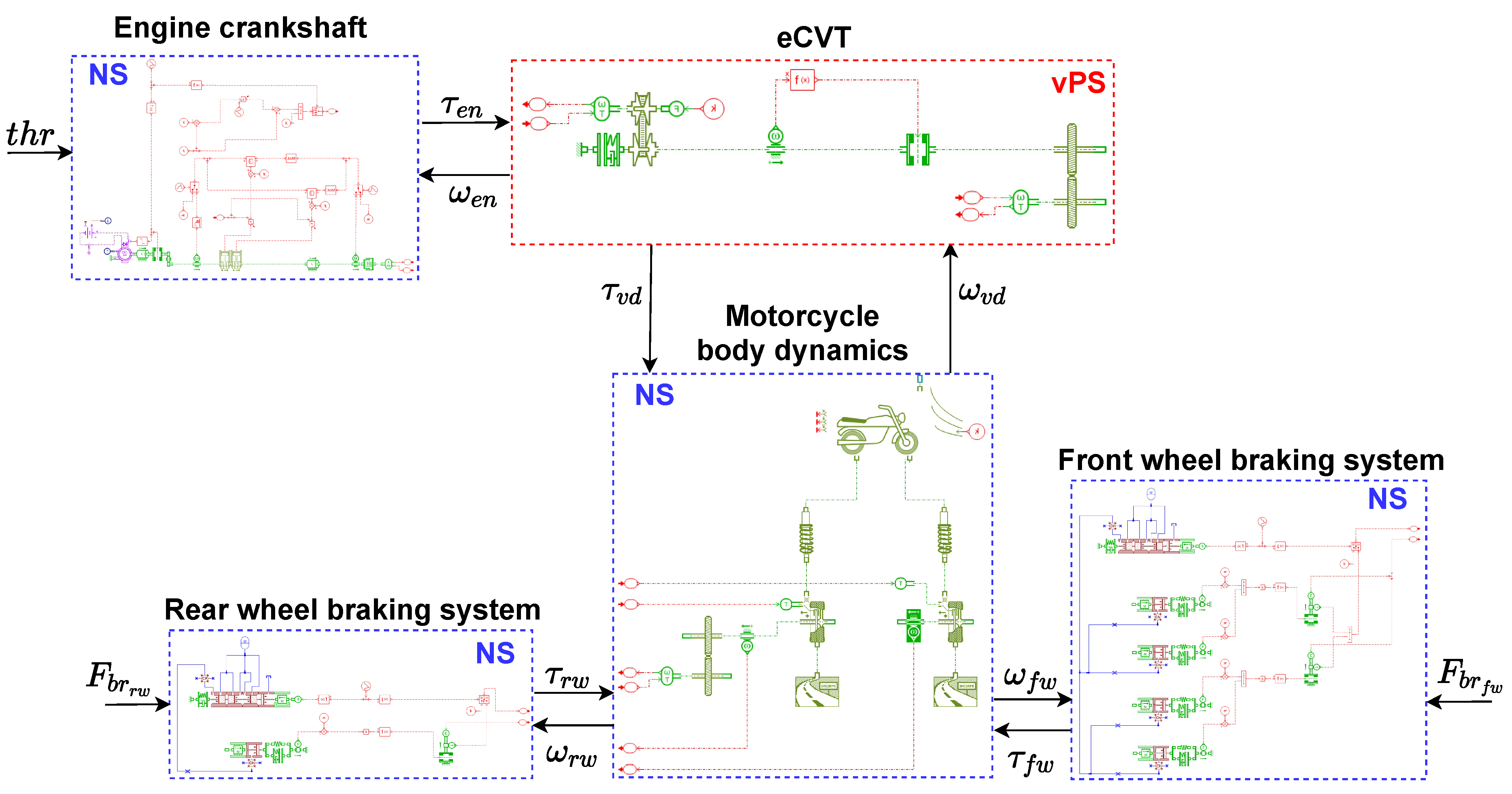
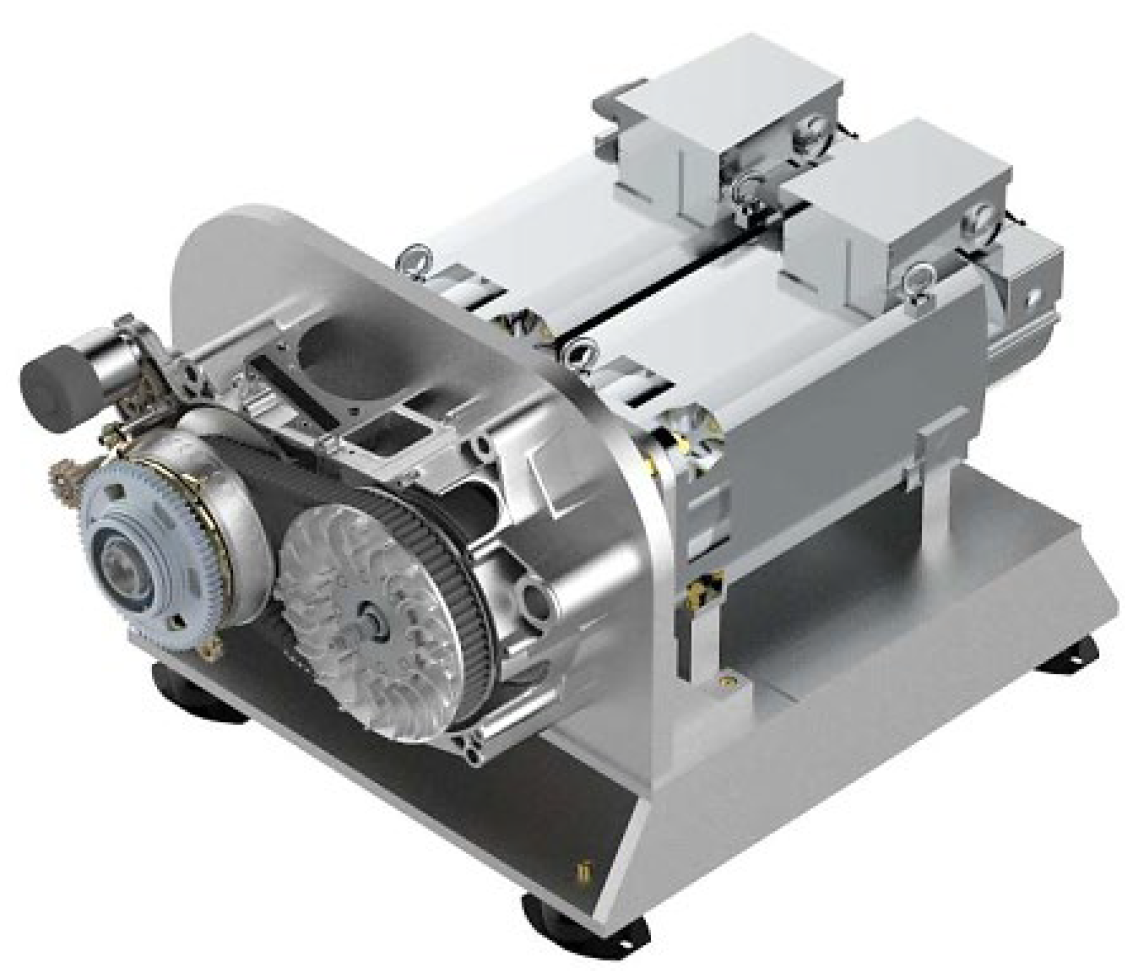
Recall from Equation (4) that the PCE of $\mathcal{M}\left(\mathit{X}\right)$ admits

$${\mathcal{M}}^{PCE}\left(\mathit{X}\right)=\sum _{\mathbf{\alpha }\in \mathcal{A}}{y}_{\mathbf{\alpha }}{\Psi }_{\mathbf{\alpha }}\left(\mathit{X}\right).$$

(33)

Due to the orthonormality of the PCE basis, the mean and variance of ${\mathcal{M}}^{PCE}\left(\mathit{X}\right)$ can be computed analytically from the $\mathit{y}$ coefficients at no extra cost, and follow [20]

$$\begin{array}{cc}\hfill \widehat{\mu }=\mathbb{E}\left[{\mathcal{M}}^{PCE}\left(\mathit{X}\right)\right]& =\mathbb{E}\left[\sum _{\mathbf{\alpha }\in \mathcal{A}}{y}_{\mathbf{\alpha }}{\Psi }_{\mathbf{\alpha }}\left(\mathit{X}\right)\right]=y_0\hfill \end{array}$$

(34)

$$\begin{array}{cc}\hfill {\widehat{\sigma }}^2=\mathrm{Var}\left[{\mathcal{M}}^{PCE}\left(\mathit{X}\right)\right]& =\mathbb{E}\left[{\left({\mathcal{M}}^{PCE}\left(\mathit{X}\right)-y_0\right)}^2\right]=\sum _{\begin{array}{c}\mathbf{\alpha }\in \mathcal{A}\\ \mathbf{\alpha }\ne \mathbf{0}\end{array}}{y}_{\mathbf{\alpha }}^2.\hfill \end{array}$$

(35)

The above equations hold since ${\Psi }_0\equiv 1$. Therefore, for the case that a PCE of Y is already constructed, the Sobol’–Hoeffding decomposition of Equation (24) can be rewritten as

$${\mathcal{M}}^{PCE}\left(\mathit{X}\right)=y_0+\sum _{\begin{array}{c}\mathsf{u}\subset \{1,\dots ,N\}\\ \mathsf{u}\ne \varnothing \end{array}}{\mathcal{M}}_{\mathit{u}}^{PCE}\left({\mathit{X}}_{\mathit{u}}\right),$$

(36)

where ${\mathcal{A}}_{\mathit{u}}=\{\mathbf{\alpha }\in \mathcal{A}:{\alpha }_m\ne 0\mathrm{if}\mathrm{and}\mathrm{only}\mathrm{if}m\in \mathit{u}\}$ corresponds to the set of multi-indices including only $\mathit{u}$ and ${\mathcal{M}}_{\mathit{u}}^{PCE}\left({\mathit{X}}_{\mathit{u}}\right)={\sum }_{\mathbf{\alpha }\in {\mathcal{A}}_{\mathit{u}}}{y}_{\mathbf{\alpha }}{\Psi }_{\mathbf{\alpha }}\left({\mathit{X}}_{\mathit{u}}\right)$, as in Equation (33). Thus, because the Sobol’–Hoeffding decomposition is unique, there exists an analytical representation of ${\mathcal{M}}_{\mathit{u}}^{PCE}$ [19]. Accordingly to Equations (34) and (35), the total and partial variances of ${\mathcal{M}}^{PCE}\left(\mathit{X}\right)$ admit

$$\begin{array}{cc}\hfill D& =\mathrm{Var}\left[{\mathcal{M}}^{PCE}\left(\mathit{X}\right)\right]=\sum _{\mathbf{\alpha }\in \mathcal{A}}{y}_{\mathbf{\alpha }}^2\hfill \\ \hfill D_{\mathit{u}}& =\mathrm{Var}\left[{\mathcal{M}}_{\mathit{u}}^{PCE}\left(\mathit{X}\right)\right]=\sum _{\mathbf{\alpha }\in {\mathcal{A}}_{\mathit{u}}}{y}_{\mathbf{\alpha }}^2.\hfill \end{array}$$

(37)

Hence, the first-order and total Sobol’ indices are obtained from

$$\begin{array}{cc}\hfill S_i^{\left(1\right)}& =\frac{{\sum }_{\mathbf{\alpha }\in {\mathcal{A}}_i}{y}_{\mathbf{\alpha }}^2}{{\sum }_{\mathbf{\alpha }\in \mathcal{A}}{y}_{\mathbf{\alpha }}^2},{\mathcal{A}}_i=\left\{\mathbf{\alpha }\in \mathcal{A}:{\alpha }_i>0,{\alpha }_{i\ne j}=0\right\}\hfill \\ \hfill S_{T_i}& =\frac{{\sum }_{\mathbf{\alpha }\in {\mathcal{A}}_i^T}{y}_{\mathbf{\alpha }}^2}{{\sum }_{\mathbf{\alpha }\in \mathcal{A}}{y}_{\mathbf{\alpha }}^2},{\mathcal{A}}_i^T=\left\{\mathbf{\alpha }\in \mathcal{A}:{\alpha }_i>0\right\},\hfill \end{array}$$

(38)

respectively. Therefore, the Sobol’ indices can be obtained as a byproduct of the PCE coefficients at no extra cost [19].

4. Case Study

This case study employs a virtual hybrid model to conduct the respective HS. Therefore, a virtual PS (vPS) is utilized instead of physical specimen, and the overall HS is performed numerically, resulting, thus, in a virtual HS (vHS).

The hybrid model represents a prototype motorcycle. It consists of one vPS, the electronically controlled continuously variable transmission (eCVT) of the motorcycle, and four NS, namely (i) the engine, (ii) the motorcycle body dynamics, (iii) the rear wheel braking system and (iv) the front wheel braking system. Figure 1 depicts how the NS and vPS are interconnected, forming the hybrid model.

The eCVT vPS is a multiple-input-multiple-output (MIMO) model, including two sets of one input and one output each. The first set is interconnected to the motorcycle engine NS, which simulates the dynamics of the combustion engine, and the second set to the motorcycle body NS. The latter connection represents the motorcycle’s transmission output shaft. The motorcycle body NS includes the motorcycle’s body/chassis dynamics along with the dynamics of the wheels, tires and suspensions. The profile of the road, as well as the environmental driving conditions, are also included in this NS. The engine NS is expressed by a multiple-input-single-output (MISO) model. Its inputs are the throttle percentage $thr$ and the angular velocity of the engine ${\omega }_{en}$, whereas its output is the torque of the engine ${\tau }_{en}$. The motorcycle body NS is expressed by a MIMO model, which includes three sets of one input and one output each. The first set of input/output is the torque ${\tau }_{vd}$ and angular velocity ${\omega }_{vd}$ of the transmission output shaft, respectively. The last two sets are connected to the rear and front wheel braking systems NS, respectively. The latter NS are both MISO models. In detail, the inputs of the rear wheel braking system NS are the angular velocity of the rear wheel ${\omega }_{rw}$ and the applied force on the brake pedal $F_{b{r}_{rw}}$, whereas its output is the braking torque of the rear wheel ${\tau }_{rw}$. Accordingly, the inputs of the front wheel braking system NS are the angular velocity of the front wheel ${\omega }_{fw}$ and the applied force on the brake lever $F_{b{r}_{fw}}$, whereas its output is the braking torque of the front wheel ${\tau }_{fw}$. The aforementioned substructures are developed using the multi-physics simulation software Simcenter Amesim. The report of [41] provides a detailed description of the development of these substructures, explaining the equations that govern their motion. Figure 2 depicts the real eCVT PS, located at the testing facilities of Siemens Industry Software, that would be utilized in a non-virtual HS.

To examine the performance of the motorcycle prototype, testing of its virtual hybrid model under predefined driving, road and wind scenarios takes place. To co-simulate the employed substructures and to coordinate the overall vHS algorithm, the Simcenter real-time platform is utilized. For the time integration scheme of the vHS, the fourth-order Runge–Kutta (RK4) method is used with a fixed time-step of 0.1 milliseconds.

The simulation duration of the case study is 45 s long, on a given driving scenario and wind/road conditions. In particular, the driving scenario is defined by the variations of the throttle $thr$ and of the forces applied to the brakes. It is assumed that the force applied in the brake lever is equal to the force applied in the brake pedal of the motorcycle in each time step of the vHS, namely $F_{b{r}_{rw}}=F_{b{r}_{fw}}$. Equations (39) and (40) describe the values that the throttle and braking forces obtain in each time step of the simulation, while Figure 3 illustrates their variations in time. It should be noted that the maximum applied throttle is $0.5$ (50%), which corresponds to a half-open throttle, and the braking forces are expressed in newtons. Equation (41) describes the road profile, namely, the height of the ground, that is assumed in this case study. It is expressed by the sinusoidal function $h\left(x\right)$, where x denotes the current position of the motorcycle in meters. Additionally, the ambient wind velocity is considered to be zero.

$$\begin{array}{c}thr\left(t\right)=\left\{\begin{array}{cc}0.125t\hfill & ,5\le t<9\hfill \\ 0.5\hfill & ,9\le t\le 13\hfill \\ -0.125t\hfill & ,13<t\le 17\hfill \\ 0\hfill & ,\mathrm{elsewhere}\hfill \end{array}\right.\end{array}$$

(39)

$$\begin{array}{c}{F}_{b{r}_{rw}}\left(t\right)=\left\{\begin{array}{cc}10t\hfill & ,20\le t<25\hfill \\ 50\hfill & ,25\le t\le 32\hfill \\ -10t\hfill & ,32<t\le 37\hfill \\ 0\hfill & ,\mathrm{elsewhere}\hfill \end{array}\right.\end{array}$$

(40)

$$\begin{array}{c}h\left(x\right)=\left\{\begin{array}{cc}0\hfill & ,0\le x\le 2\hfill \\ 0.02\left(cos\left(\frac{2\pi x}{3}\right)-1\right)\hfill & ,\mathrm{elsewhere}\hfill \end{array}\right.\end{array}$$

(41)

For the GSA, two hybrid model response QoI are selected, namely, the maximum $v_{\max }$ and mean $v_{\mathrm{mean}}$ values of the motorcycle velocity. Both QoI are expressed in km/h. Scalar quantities from the dynamic response of the motorcycle’s velocity are chosen in particular since the latter is a global response parameter that can characterize the overall dynamic behavior of the hybrid model of the prototype motorcycle. In addition, the input variables to GSA are the 12 parameters which are listed in

Table 1. Input variables of the hybrid model for GSA and their probability distributions.

Param.	Prob. Distrib.	Mean Value	Stand. Dev.	CV (%)	Parameter Description	Units
$K_{rt}$	Unif.	58,570	11,714	20	Vertical stiffness rear tire	$\frac{\mathrm{N}}{\mathrm{m}}$
$Z_{rt}$	Unif.	11,650	3495	30	Vertical damping rear tire	$\frac{\mathrm{N}\mathrm{s}}{\mathrm{m}}$
$K_{ft}$	Unif.	25,000	5000	20	Vertical stiffness front tire	$\frac{\mathrm{N}}{\mathrm{m}}$
$Z_{ft}$	Unif.	2134	$640.2$	30	Vertical damping front tire	$\frac{\mathrm{N}\mathrm{s}}{\mathrm{m}}$
$K_{rs}$	Unif.	125,000	25,000	20	Stiffness rear suspension	$\frac{\mathrm{N}}{\mathrm{m}}$
$Z_{rs}$	Unif.	10,000	3000	30	Damping rear suspension	$\frac{\mathrm{N}\mathrm{s}}{\mathrm{m}}$
$K_{fs}$	Unif.	19,000	3800	20	Stiffness front suspension	$\frac{\mathrm{N}}{\mathrm{m}}$
$Z_{fs}$	Unif.	1250	375	30	Damping front suspension	$\frac{\mathrm{N}\mathrm{s}}{\mathrm{m}}$
M	Unif.	300	15	5	Motorcycle mass	$\genfrac{}{}{0.0pt}{}{\mathrm{Kg}}{}$
J	Unif.	$0.0115$	$0.0023$	20	Engine moment of inertia	$\genfrac{}{}{0.0pt}{}{{\mathrm{Kgm}}^2}{}$
$E\mu$	Unif.	$0.0012$	$0.00018$	15	Engine coefficient of viscous friction	$\frac{\mathrm{Nm}}{\mathrm{rev}/\min }$
$B\mu$	Unif.	$0.13$	$0.0195$	15	Brake coefficient of viscous friction	$\frac{\mathrm{Nm}}{\mathrm{rad}/\mathrm{s}}$

. The probability distributions that are assigned to each parameter along with their respective moments are also presented in Table 1. The bounds of each parameter are identified from [42,43,44,45] to reflect a range of possible parameter variations of the corresponding motorcycle components. According to the notation presented in Section 2 and Section 3, the experimental design (ED) vectors for this case study follow

$$\begin{array}{c}\begin{array}{c}\mathit{X}=\{K_{rt},Z_{rt},K_{ft},Z_{ft},K_{rs},Z_{rs},K_{fs},Z_{fs},M,J,E\mu ,B\mu \}\\ \mathit{Y}=\{v_{\max },v_{\mathrm{mean}}\},\end{array}\end{array}$$

(42)

From the input parameters of Table 1, 200 points are generated using the Latin hypercube sampling (LHS) method [46], and accordingly, 200 vHS are conducted, collecting the QoI values in the $\mathit{Y}$ vector of Equation (42). With the obtained data in ED$\{\mathit{X},\mathit{Y}\}$, a PCE, a Kriging and a PCK surrogate are developed for each QoI, as described in Section 2.1, Section 2.2 and Section 2.3, respectively. Figure 4 illustrates a sample vHS time history response of the hybrid model, indicating the QoI of the case study, which are highlighted in red color. Additionally, Figure 5 depicts some indicative dynamic responses of the variables that couple the substructures in the virtual hybrid model. The responses in the latter two figures are obtained using the mean, i.e., nominal, values of Table 1, while the hybrid model is excited with the driving scenario, the road profile and wind conditions that are described by Equations (39)–(41).

In addition, the time history responses of Figure 4 and Figure 5 can be intuitively interpreted. Figure 5b shows the response of the front wheel braking torque ${\tau }_{fw}$, generated by the utilized driving scenario. Recall from Figure 3 and Equation (40) that the brakes of the motorcycle are enabled in the time interval between the 20th and 37th second of the simulation and as a result, the braking torques are non-zero only then. According to Figure 3 and Equation (39), the throttle applied in the motorcycle’s engine in the five first seconds of the simulation is zero, and therefore its velocity is also zero (Figure 4). In the time interval between the 5th and 17th second of the simulation, the throttle starts to increase and hence, the motorcycle starts to accelerate. From Figure 4, it can be seen that the velocity is also increasing. After the 20th second of the simulation, the braking starts (Equation (40)) and as a result, the velocity of the motorcycle begins to decrease, while it is brought to almost a full stop in the 45th second of the simulation.

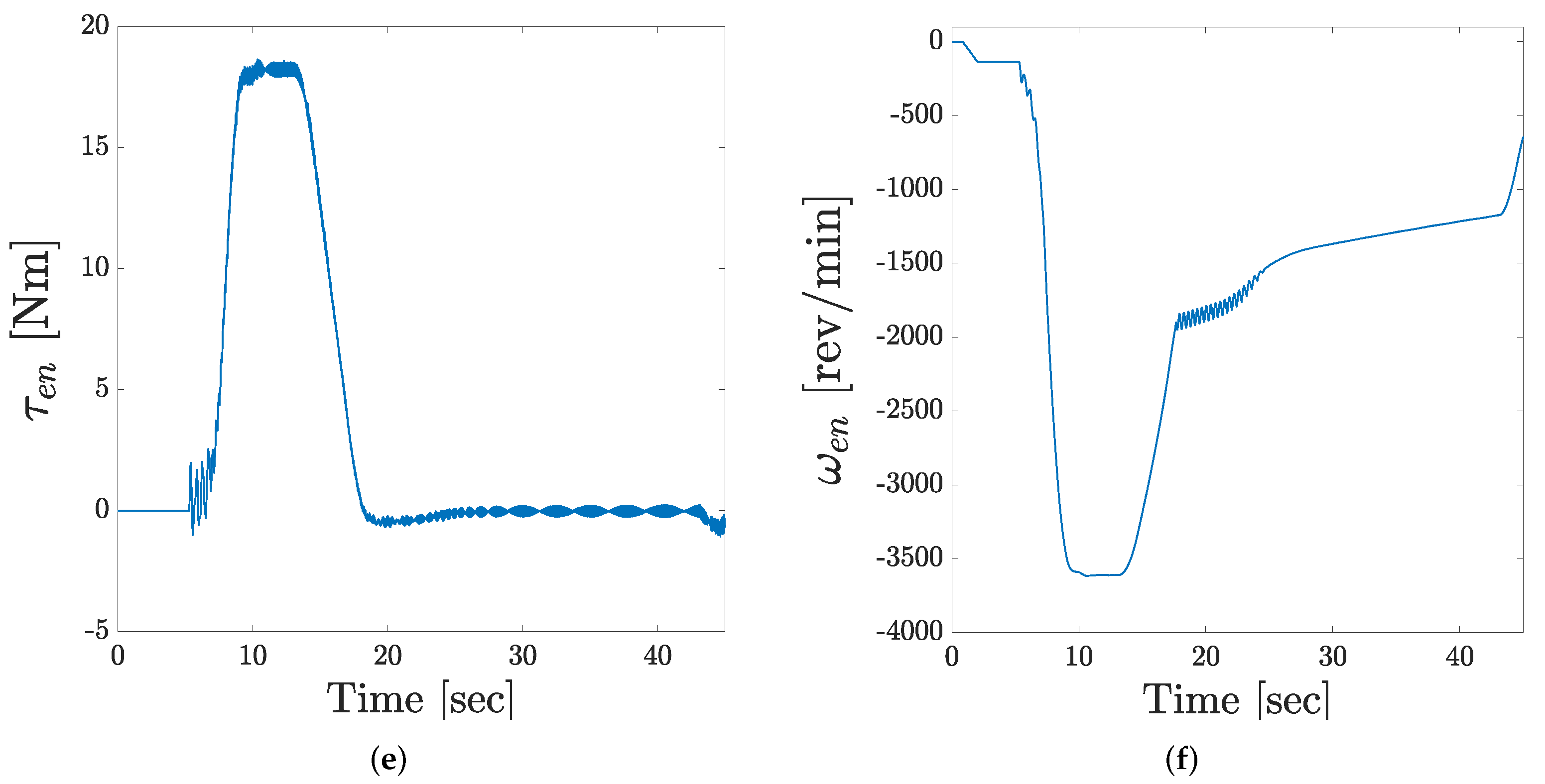
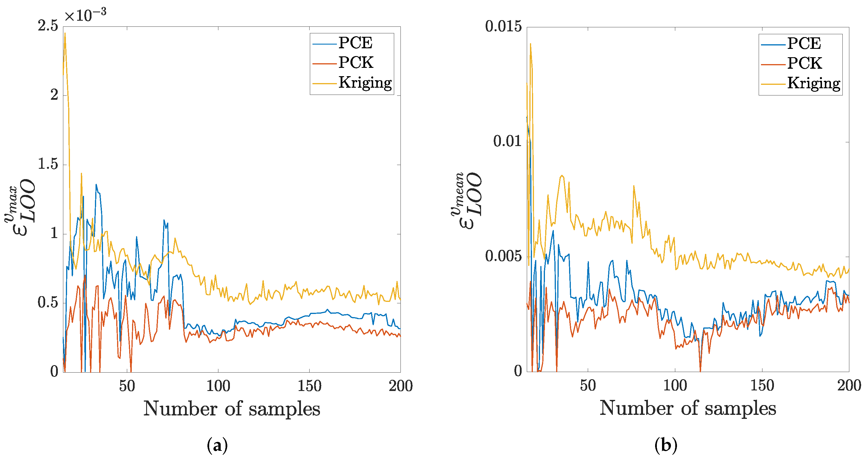
5. Results and Discussion

Figure 6 displays the convergence of the LOO errors of the PCE, PCK and Kriging surrogates for both QoI. The LOO errors are computed using EDs of increasing size from 15 to 200 samples. From Figure 6, it can be appreciated that the LOO errors of PCE and PCK are quite close, while the error of Kriging is slightly larger. Yet, all the errors are negligibly small, as they converge to values in the magnitude of ${10}^{-3}$ or smaller. The satisfying performance of the surrogates can be also confirmed from Figure 7, which illustrates validation scatter plots by comparing the measurements of the two QoI with the respective predictions from the corresponding PCE, PCK and Kriging surrogates. In more detail, for each QoI, the surrogates are trained on 150 samples of the ED, and the remaining 50 samples are used to validate them.

In addition, Figure 8 and Figure 9 depict the convergence plots of the PCE-based moments estimates, i.e., mean, standard deviation and coefficient of variation (CV) values, for both QoI. Recall that the PCE-based moments estimates can be computed from the PCE coefficients as a post-process at no additional computational cost [19]. However, the latter is not a feature of Kriging or PCK. Thus, Figure 8 and Figure 9 do not include moment estimates from these two surrogates. Nevertheless, to further evaluate the performance of the developed surrogates, Figure 10 compares the prediction PDF of each surrogate against the histograms of the measurements for each QoI. The surrogate predictions are evaluated based on 200 random samples, generated from the distributions described in Table 1 using the LHS method. From Figure 10, it can be acknowledged that all three developed surrogates can capture quite well both the mean value and the variance of the corresponding measurements.

From Figure 6, Figure 7 and Figure 10, it can be appreciated that the performance and accuracy prediction of PCE, PCK and Kriging are similar. However, it should be noted that the computational time associated to train each surrogate differs. For the case of PCE and Kriging, the training computational times are approximately $6.1$ and $7.5$ s, respectively. Nevertheless, for the case of PCK, it is approximately 38 s. The latter finding can be intuitively interpreted, as in the PCK case, the training phase consists of two steps: one constructing the PCE and a second one to determine the Kriging model. Note that these timings depend heavily on the ED sample size as well as on the settings for which each surrogate is developed.

Once the surrogates of each QoI are developed, the Sobol’ indices can be computed. For the case of PCE, the Sobol’ indices are computed analytically at no extra cost [19], as described in Section 3.3.2. For the cases of PCK and Kriging, though, this is not possible; thus the Sobol’ indices are computed using Monte Carlo evaluations of the surrogate response QoI, as described in Section 3.3.1. It should be noted that more than ${10}^4$ Monte Carlo evaluations of the Kriging and PCK surrogates are needed to ensure convergence of the Sobol’ indices. In this case study, ${10}^5$ evaluations of the response QoI of the Kriging and PCK surrogates are performed to compute the respective Sobol’ indices. However, it is worth mentioning that the computational cost of running these evaluations is negligibly small (≈1 s for each surrogate).

In Figure 11 the first-order and total Sobol’ indices for both QoI $v_{\max }$ and $v_{\mathrm{mean}}$ are reported. Clearly, both first-order and total Sobol’ indices computed utilizing the different examined surrogates are admittedly close with each other. This confirms that the indices obtained from the PCK and Kriging converge to the analytical values computed from the PCE coefficients. From Figure 11, it can be stated that the input variables related to the motorcycle mass M as well as to the engine coefficient of viscous friction $E\mu$ are the most sensitive variables for both QoI. In particular, for the QoI related to the maximum motorcycle velocity, namely, $v_{\max }$, the motorcycle mass has a greater effect than the engine friction coefficient, whereas, for the QoI related to the mean motorcycle velocity, namely $v_{\mathrm{mean}}$, the engine friction coefficient contributes more than the motorcycle mass. On the contrary, the remaining input variables of Table 1 do not affect significantly the selected QoI. Furthermore, since the first-order and total Sobol’ indices for both QoI are quite close, it can be noticed that the effect from high-order interactions between the input variables is negligible.

The development and implementation of the surrogate modeling, as well as the GSA, are performed with the UQLab software framework developed by the Chair of Risk, Safety and Uncertainty Quantification in ETH Zurich [47].

6. Conclusions

This paper shows how different surrogate modeling methods can be used to perform global sensitivity analysis via Sobol’ indices in hybrid simulation. Global sensitivity analysis using Sobol’ indices is established as a powerful tool to unveil the sensitivity of a structural system, i.e., its hybrid model, subjected to parameter and loading variations. However, estimation of the Sobol’ indices through Monte Carlo simulations of the original hybrid model is rarely affordable since many hybrid model evaluations are essential, while each evaluation relies on a single hybrid simulation. To alleviate this burden, surrogate models of selected hybrid model response quantities of interest can be constructed and used to estimate the Sobol’ indices at a much lower cost. A case study encompassing a virtual hybrid model is employed to investigate this approach by using a variety of different surrogate modeling techniques. In this regard, polynomial chaos expansion, Kriging (i.e., Gaussian process) and polynomial chaos Kriging are used to develop surrogates of the selected quantities of interest. For the case of polynomial chaos expansion, the Sobol’ indices are computed as a by-product of the polynomial coefficients, and hence, no additional computational cost is required. However, the latter is not a feature of Kriging and polynomial chaos Kriging. Therefore, Monte Carlo simulations using these surrogates are performed to estimate the Sobol’ indices. Performance comparisons between each developed surrogate indicate that the respective validation errors were similar. Additionally, negligibly small deviations are observed in the Sobol’ indices obtained using the different surrogate modeling techniques. Future work aims at adaptive sampling of the input parameter space of the hybrid model to minimize the experimentation cost necessary to compute an accurate surrogate model for global sensitivity analysis.

References

1. Tsokanas, N.; Wagg, D.; Stojadinović, B. Robust Model Predictive Control for Dynamics Compensation in Real-Time Hybrid Simulation. Front. Built Environ. 2020, 6, 127. [Google Scholar] [CrossRef]
2. Tsokanas, N.; Pastorino, R.; Stojadinovic, B. Adaptive model predictive control for actuation dynamics compensation in real-time hybrid simulation. engrXiv 2021. [Google Scholar] [CrossRef]
3. Li, H.; Maghareh, A.; Montoya, H.; Condori Uribe, J.W.; Dyke, S.J.; Xu, Z. Sliding mode control design for the benchmark problem in real-time hybrid simulation. Mech. Syst. Signal Process. 2021, 151, 107364. [Google Scholar] [CrossRef]
4. Simpson, T.; Dertimanis, V.K.; Chatzi, E.N. Towards Data-Driven Real-Time Hybrid Simulation: Adaptive Modeling of Control Plants. Front. Built Environ. 2020, 6, 158. [Google Scholar] [CrossRef]
5. Tsokanas, N.; Simpson, T.; Pastorino, R.; Chatzi, E.; Stojadinovic, B. Model Order Reduction for Real-Time Hybrid Simulation: Comparing Polynomial Chaos Expansion and Neural Network methods. engrXiv 2021. [Google Scholar] [CrossRef]
6. Miraglia, G.; Petrovic, M.; Abbiati, G.; Mojsilovic, N.; Stojadinovic, B. A model-order reduction framework for hybrid simulation based on component-mode synthesis. Earthq. Eng. Struct. Dyn. 2020, 49, 737–753. [Google Scholar] [CrossRef]
7. Schellenberg, A.H.; Mahin, S.A.; Fenves, G.L. Advanced Implementation of Hybrid Simulation; Technical Report PEER 2009/104; Pacific Earthquake Engineering Research Center, University of California: Berkeley, CA, USA, 2009. [Google Scholar]
8. Tsokanas, N. Real-Time and Stochastic Hybrid Simulation. Ph.D. Thesis, ETH Zurich, Zurich, Switzerland, 2021. [Google Scholar] [CrossRef]
9. Abbiati, G.; Lanese, I.; Cazzador, E.; Bursi, O.S.; Pavese, A. A computational framework for fast-time hybrid simulation based on partitioned time integration and state-space modeling. Struct. Control Health Monit. 2019, 26, e2419. [Google Scholar] [CrossRef]
10. Abbiati, G.; Covi, P.; Tondini, N.; Bursi, O.S.; Stojadinović, B. A Real-Time Hybrid Fire Simulation Method Based on Dynamic Relaxation and Partitioned Time Integration. J. Eng. Mech. 2020, 146, 04020104. [Google Scholar] [CrossRef]
11. Song, W.; Sun, C.; Zuo, Y.; Jahangiri, V.; Lu, Y.; Han, Q. Conceptual Study of a Real-Time Hybrid Simulation Framework for Monopile Offshore Wind Turbines Under Wind and Wave Loads. Front. Built Environ. 2020, 6, 129. [Google Scholar] [CrossRef]
12. Idinyang, S.; Franza, A.; Heron, C.M.; Marshall, A.M. Real-time data coupling for hybrid testing in a geotechnical centrifuge. Int. J. Phys. Model. Geotech. 2018, 19, 208–220. [Google Scholar] [CrossRef]
13. Tsokanas, N.; Abbiati, G.; Kanellopoulos, K.; Stojadinovic, B. Multi-Axial Hybrid Fire Testing based on Dynamic Relaxation. Fire Saf. J. 2021, 126, 103468. [Google Scholar] [CrossRef]
14. Tsokanas, N.; Stojadinovic, B. A stochastic real-time hybrid simulation of the seismic response of a magnetorheological damper. In Proceedings of the 17th World Conference on Earthquake Engineering (17WCEE 2020), Sendai, Japan, 13–18 September 2020. [Google Scholar] [CrossRef]
15. Tsokanas, N.; Stojadinovic, B. Design of an Actuation Controller for Physical Substructures in Stochastic Real-Time Hybrid Simulations. In Model Validation and Uncertainty Quantification; Mao, Z., Ed.; Society for Experimental Mechanics Series; Springer International Publishing: Cham, Switzerland, 2020; Volume 3, pp. 69–82. [Google Scholar] [CrossRef]
16. Abbiati, G.; Marelli, S.; Tsokanas, N.; Sudret, B.; Stojadinović, B. A global sensitivity analysis framework for hybrid simulation. Mech. Syst. Signal Process. 2021, 146, 106997. [Google Scholar] [CrossRef]
17. Tsokanas, N.; Zhu, X.; Abbiati, G.; Marelli, S.; Sudret, B.; Stojadinović, B. A Global Sensitivity Analysis Framework for Hybrid Simulation with Stochastic Substructures. Front. Built Environ. 2021, 7, 154. [Google Scholar] [CrossRef]
18. Saltelli, A.; Ratto, M.; Andres, T.; Campolongo, F.; Cariboni, J.; Gatelli, D.; Saisana, M.; Tarantola, S. Global Sensitivity Analysis. The Primer; John Wiley & Sons, Ltd.: Chichester, UK, 2007; Volume 76. [Google Scholar]
19. Sudret, B. Global sensitivity analysis using polynomial chaos expansions. Reliab. Eng. Syst. Saf. 2008, 93, 964–979. [Google Scholar] [CrossRef]
20. Le Gratiet, L.; Marelli, S.; Sudret, B. Metamodel-Based Sensitivity Analysis: Polynomial Chaos Expansions and Gaussian Processes. In Handbook of Uncertainty Quantification; Ghanem, R., Higdon, D., Owhadi, H., Eds.; Springer International Publishing: Cham, Switzerland, 2017; pp. 1289–1325. [Google Scholar]
21. Ghanem, R.; Spanos, P.D. Polynomial Chaos in Stochastic Finite Elements. J. Appl. Mech. 1990, 57, 197–202. [Google Scholar] [CrossRef]
22. Xiu, D.; Karniadakis, G.E. The Wiener–Askey Polynomial Chaos for Stochastic Differential Equations. SIAM J. Sci. Comput. 2002, 24, 619–644. [Google Scholar] [CrossRef]
23. Spiridonakos, M.D.; Chatzi, E.N. Metamodeling of dynamic nonlinear structural systems through polynomial chaos NARX models. Comput. Struct. 2015, 157, 99–113. [Google Scholar] [CrossRef]
24. Torre, E.; Marelli, S.; Embrechts, P.; Sudret, B. Data-driven polynomial chaos expansion for machine learning regression. J. Comput. Phys. 2019, 388, 601–623. [Google Scholar] [CrossRef] [Green Version]
25. Marelli, S.; Sudret, B. UQLab User Manual—Polynomial Chaos Expansions; Technical Report # UQLab-V1.3-104; Risk, Safety and Uncertainty Quantification, ETH Zurich: Zurich, Switzerland, 2019. [Google Scholar]
26. Blatman, G.; Sudret, B. Adaptive sparse polynomial chaos expansion based on least angle regression. J. Comput. Phys. 2011, 230, 2345–2367. [Google Scholar] [CrossRef]
27. Berveiller, M.; Sudret, B.; Lemaire, M. Stochastic finite element: A non intrusive approach by regression. Eur. J. Comput. Mech. 2006, 15, 81–92. [Google Scholar] [CrossRef] [Green Version]
28. Eldred, M.; Webster, C.; Constantine, P. Evaluation of Non-Intrusive Approaches for Wiener-Askey Generalized Polynomial Chaos. In Proceedings of the 49th AIAA Structures, Structural Dynamics, and Materials Conference, Schaumburg, IL, USA, 7–10 April 2008. [Google Scholar]
29. Zhang, J.; Yue, X.; Qiu, J.; Zhuo, L.; Zhu, J. Sparse polynomial chaos expansion based on Bregman-iterative greedy coordinate descent for global sensitivity analysis. Mech. Syst. Signal Process. 2021, 157, 107727. [Google Scholar] [CrossRef]
30. Santner, T.J.; Williams, B.J.; Notz, W.I. The Design and Analysis of Computer Experiments; Springer Series in Statistics; Springer: New York, NY, USA, 2003. [Google Scholar]
31. Rasmussen, C.E.; Williams, C.K.I. Gaussian Processes for Machine Learning (Adaptive Computation and Machine Learning); The MIT Press: Cambridge, MA, USA, 2005. [Google Scholar]
32. Lataniotis, C.; Wicaksono, D.; Marelli, S.; Sudret, B. UQLab User Manual —Kriging (Gaussian Process Modeling); Technical Report # UQLab-V1.3-105; Risk, Safety and Uncertainty Quantification, ETH Zurich: Zurich, Switzerland, 2019. [Google Scholar]
33. Dubourg, V. Adaptive Surrogate Models for Reliability Analysis and Reliability-Based Design Optimization. Ph.D. Thesis, Université Blaise Pascal-Clermont-Ferrand II, Clermont-Ferrand, France, 2011. [Google Scholar]
34. Goldberg, D.E.; Holland, J.H. Genetic Algorithms and Machine Learning. Mach. Learn. 1988, 3, 95–99. [Google Scholar] [CrossRef]
35. Schobi, R.; Sudret, B.; Wiart, J. Polynomial-chaos-based Kriging. Int. J. Uncertain. Quantif. 2015, 5, 171–193. [Google Scholar] [CrossRef]
36. Schöbi, R.; Sudret, B.; Marelli, S. Rare Event Estimation Using Polynomial-Chaos Kriging. ASCE-ASME J. Risk Uncertain. Eng. Syst. Part A Civ. Eng. 2017, 3, D4016002. [Google Scholar] [CrossRef] [Green Version]
37. Kersaudy, P.; Sudret, B.; Varsier, N.; Picon, O.; Wiart, J. A new surrogate modeling technique combining Kriging and polynomial chaos expansions—Application to uncertainty analysis in computational dosimetry. J. Comput. Phys. 2015, 286, 103–117. [Google Scholar] [CrossRef] [Green Version]
38. Schöbi, R.; Marelli, S.; Sudret, B. UQLab User Manual—Polynomial Chaos Kriging; Technical Report # UQLab-V1.3-109; Risk, Safety and Uncertainty Quantification, ETH Zurich: Zurich, Switzerland, 2019. [Google Scholar]
39. Sobol’, I.M. Sensitivity analysis for non-linear mathematical models. Math. Model. Comput. Exp. 1993, 1, 407–414. [Google Scholar]
40. Marelli, S.; Lamas, C.; Konakli, K.; Mylonas, C.; Wiederkehr, P.; Sudret, B. UQLab User Manual—Sensitivity Analysis; Technical Report # UQLab-V1.3-106; Risk, Safety and Uncertainty Quantification, ETH Zurich: Zurich, Switzerland, 2019. [Google Scholar]
41. Pinheiro, S.M. Motorcycle Modeling for eCVT-in-the-Loop Real-Time Hybrid Testing. Master’s Thesis, University of Porto, Porto, Portugal, 2020. [Google Scholar]
42. Kimishima, T.; Nakamura, T.; Suzuki, T. The Effects on Motorcycle Behavior of the Moment of Inertia of the Crankshaft. SAE Trans. 1997, 106, 1993–2003. [Google Scholar]
43. Tanelli, M. Modelling, Simulation and Control of Two-Wheeled Vehicles; John Wiley & Sons: New, York, NY, USA, 2014. [Google Scholar]
44. Sharp, R.; Evangelou, S.; Limebeer, D. Advances in the Modelling of Motorcycle Dynamics. Multibody Syst. Dyn. 2004, 12, 251–283. [Google Scholar] [CrossRef] [Green Version]
45. Jia, S.; Li, Q. Friction-induced vibration and noise on a brake system. In Proceedings of the 2013 IEEE International Conference on Information and Automation (ICIA), Yinchuan, China, 26–28 August 2013; pp. 489–492. [Google Scholar] [CrossRef]
46. Mckay, M.D.; Beckman, R.J.; Conover, W.J. A Comparison of Three Methods for Selecting Values of Input Variables in the Analysis of Output from a Computer Code. Technometrics 2000, 42, 55–61. [Google Scholar] [CrossRef]
47. Marelli, S.; Sudret, B. UQLab: A Framework for Uncertainty Quantification in Matlab. In Proceedings of the 2nd International Conference on Vulnerability, Risk Analysis and Management (ICVRAM2014), Liverpool, UK, 13–16 July 2014; pp. 2554–2563. [Google Scholar] [CrossRef] [Green Version]
Figure 1. Motorcycle hybrid model block diagram.
Make 04 00001 g001
Figure 2. The eCVT test bench at the testing facilities of Siemens Industry Software.
Make 04 00001 g002
Figure 3. Case study driving scenario.
Make 04 00001 g003
Figure 4. Sample vHS time history response of the motorcycle prototype hybrid model, using the mean (nominal) values of Table 1. The QoI are highlighted in red color.
Make 04 00001 g004
Figure 5. Indicative hybrid model responses, using the mean (nominal) values of Table 1: (a) angular velocity of the rear wheel, (b) braking torque of the rear wheel, (c) angular velocity of the transmission output shaft, (d) torque of the transmission output shaft, (e) torque of the engine and (f) angular velocity of the engine.
Make 04 00001 g005aMake 04 00001 g005b
Figure 6. Convergence of LOO error estimates of (a) v max and (b) v mean surrogates.
Make 04 00001 g006
Figure 7. Comparison between QoI measurements and corresponding surrogate predictions for (a) v max and (b) v mean .
Make 04 00001 g007
Figure 8. Convergence of PCE-based moments estimates of (a) mean, (b) standard deviation and (c) CV of QoI v max .
Make 04 00001 g008
Figure 9. Convergence of PCE-based moments estimates of (a) mean, (b) standard deviation and (c) CV of QoI v mean .
Make 04 00001 g009
Figure 10. Comparison between histogram measurements and corresponding surrogate estimates for (a) v max and (b) v mean .
Make 04 00001 g010
Figure 11. First-order and total Sobol’ indices for (a,b) v max and (c,d) v mean .
Make 04 00001 g011