
Orientation-Encoding CNN for Point Cloud Classification and Segmentation

Abstract
:1. Introduction
- We propose a general network architecture for point cloud classification and segmentation.
- The framework is simple and effective.
- The network has certain adaptability.
- Our OE convolution and pooling strategies are perceptive to local geometric features of point sets.
2. Related Work
2.1. Point Cloud Classification and Segmentation
2.2. Voxel Data
2.3. Spatial Domain
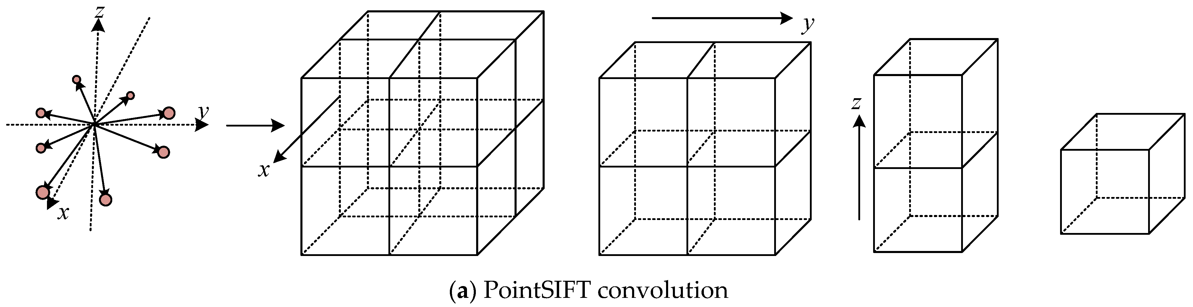
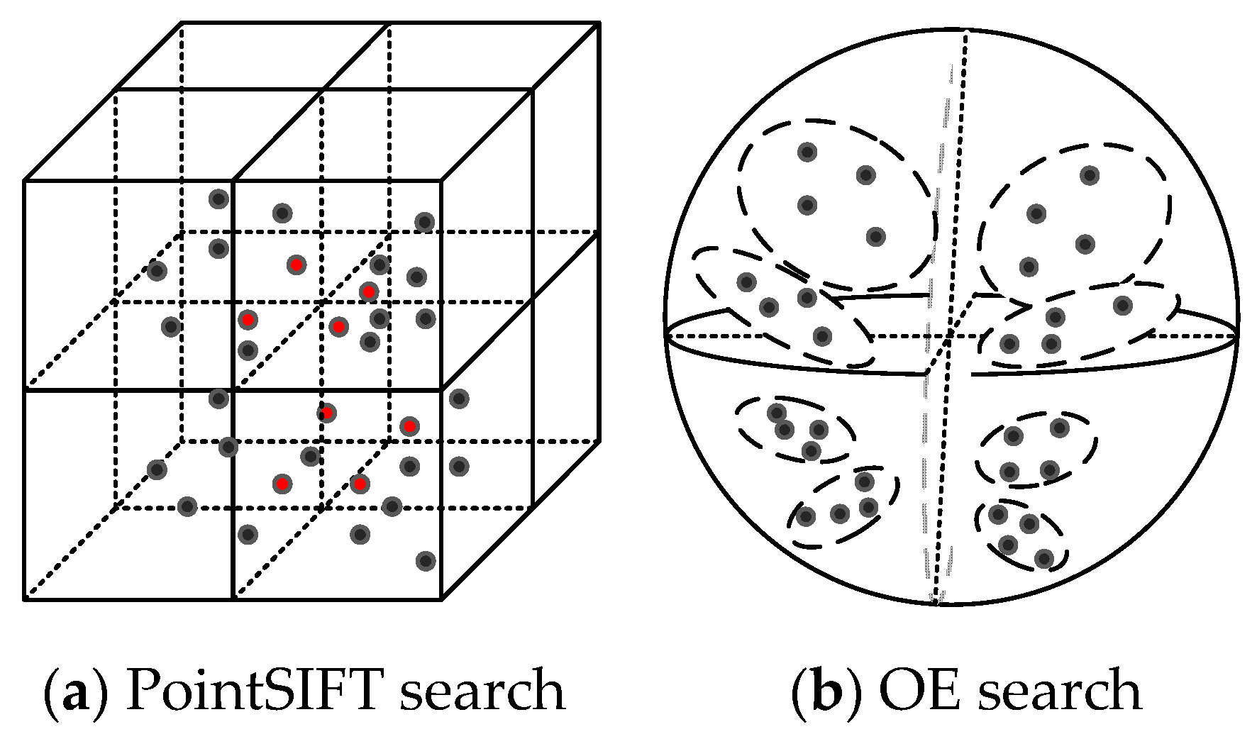
3. Method Design
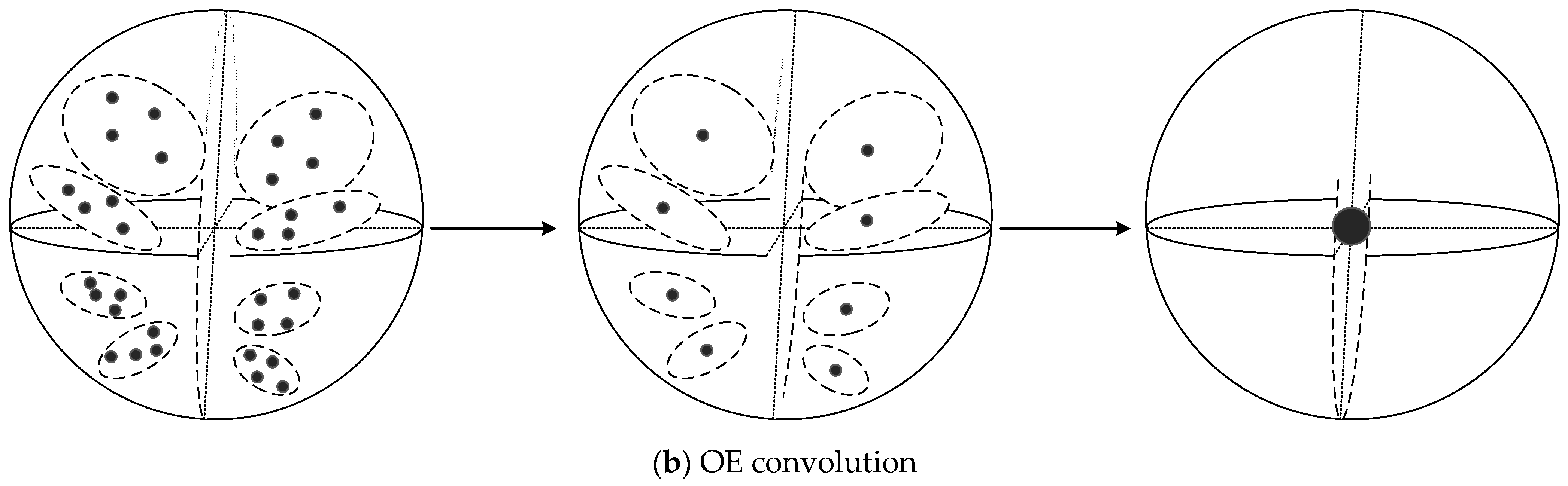
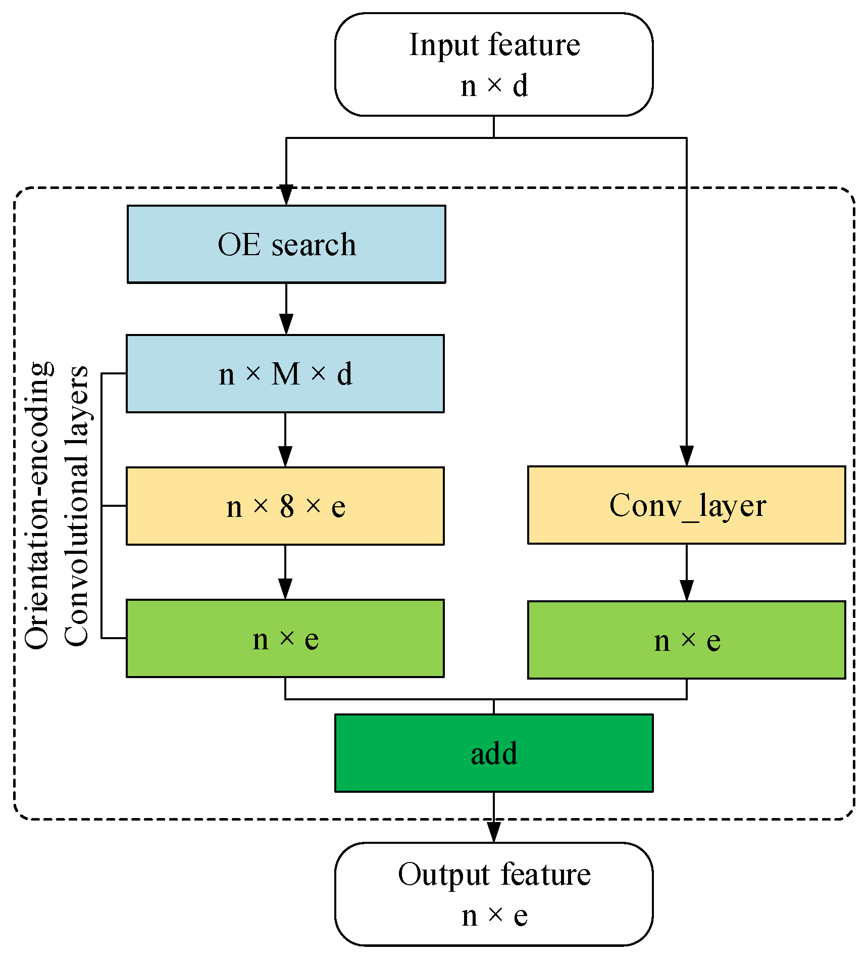
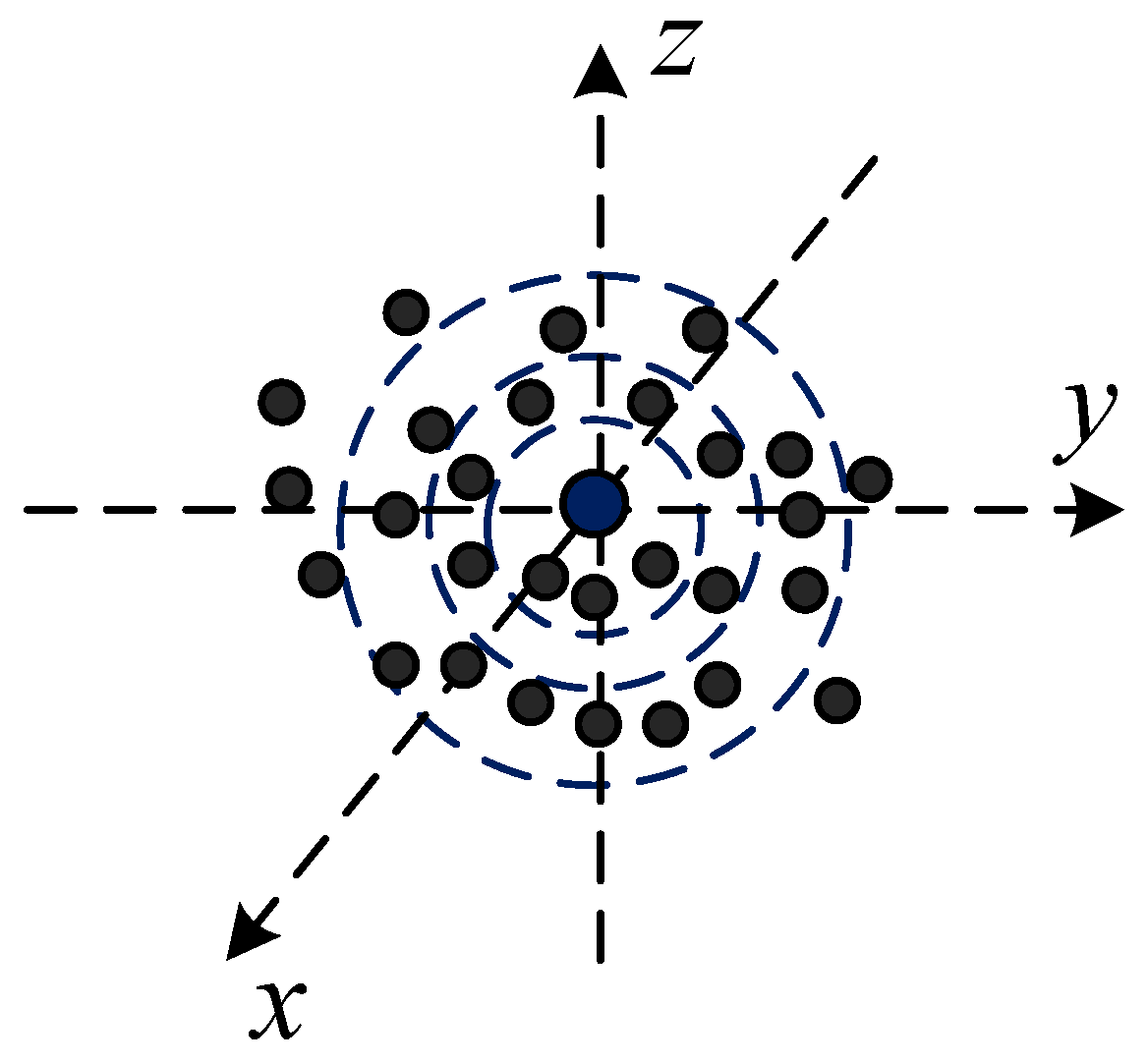
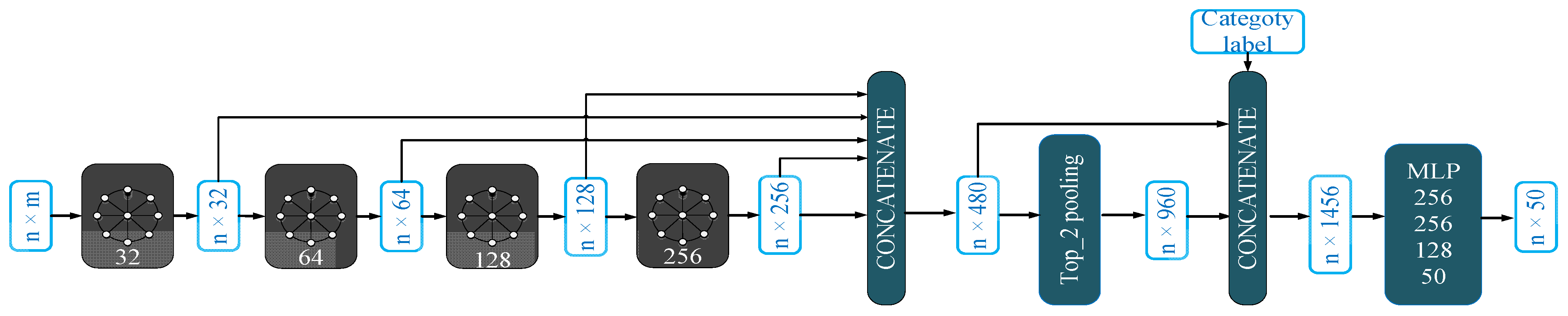
3.1. Orientation-Encoding (OE) Architecture
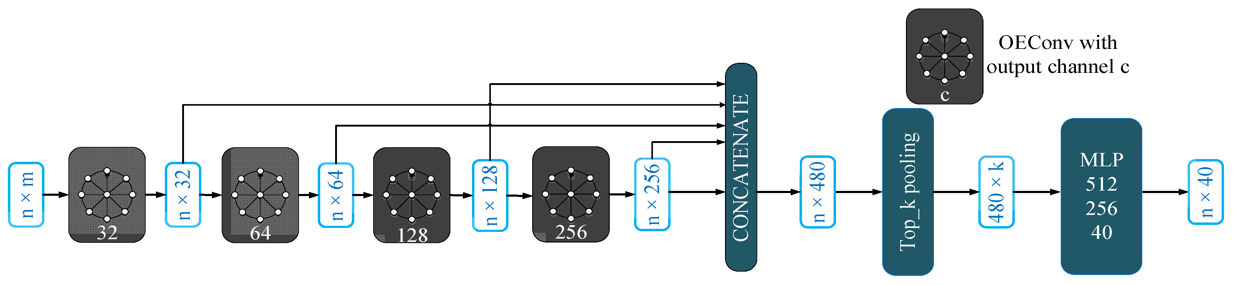
3.2. Multi-Scale Architecture
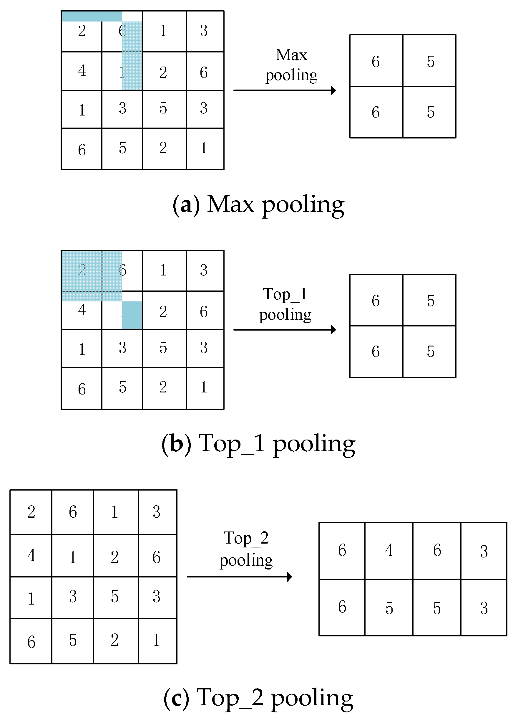
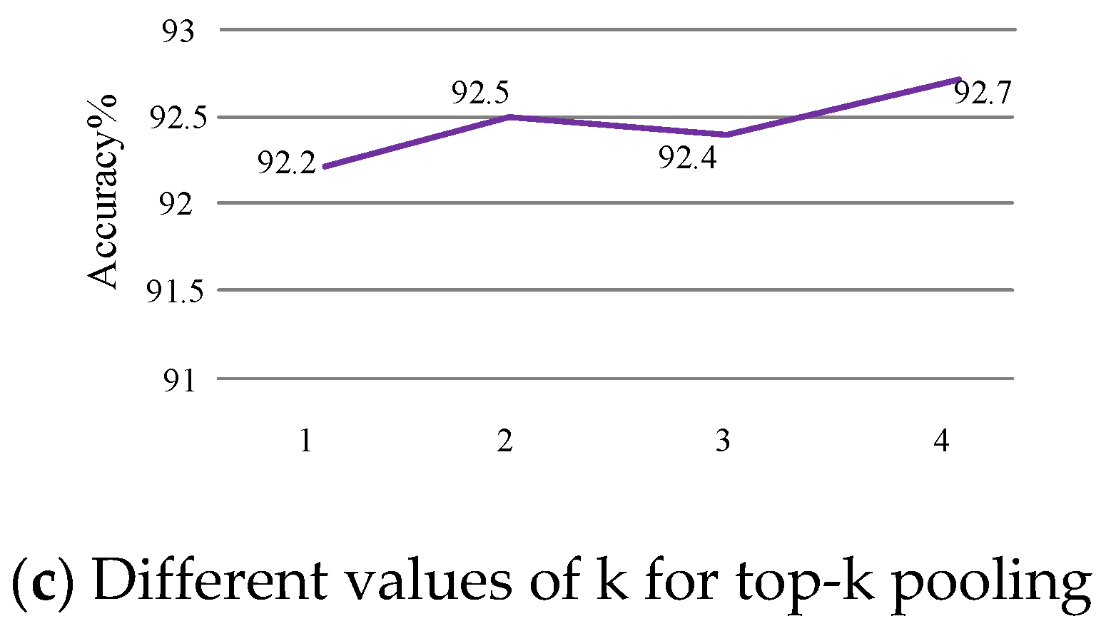
3.3. Top-k Pooling vs. Max Pooling
4. Experiment
4.1. Experimental Environment
4.2. Classification on ModelNet40
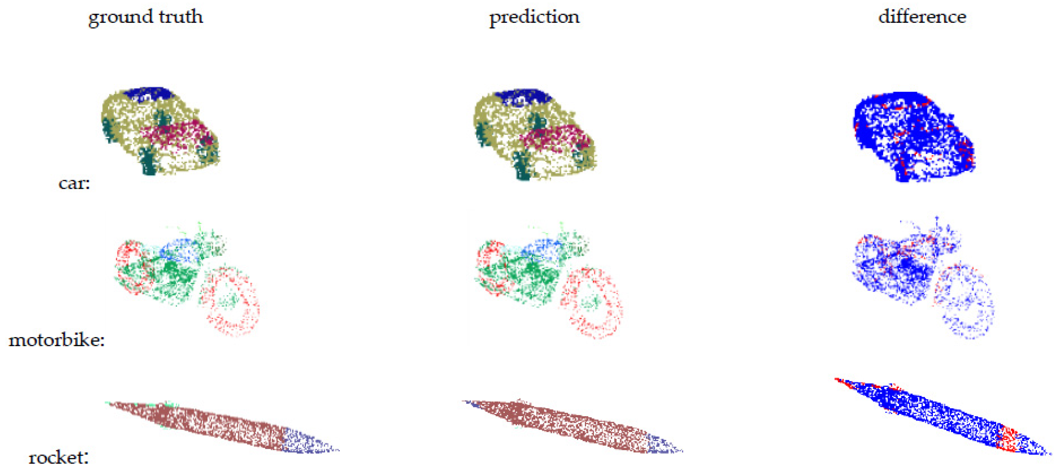
4.3. Segmentation on ShapeNet Parts
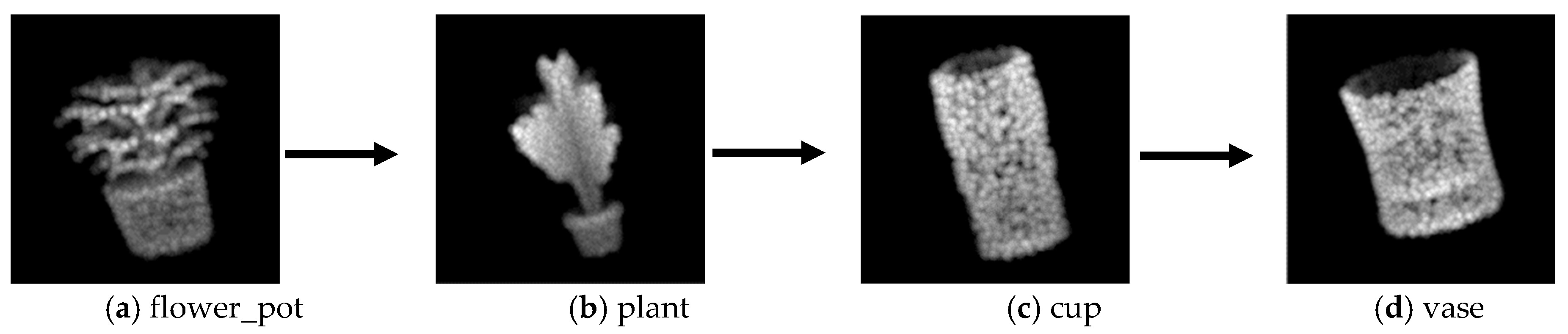
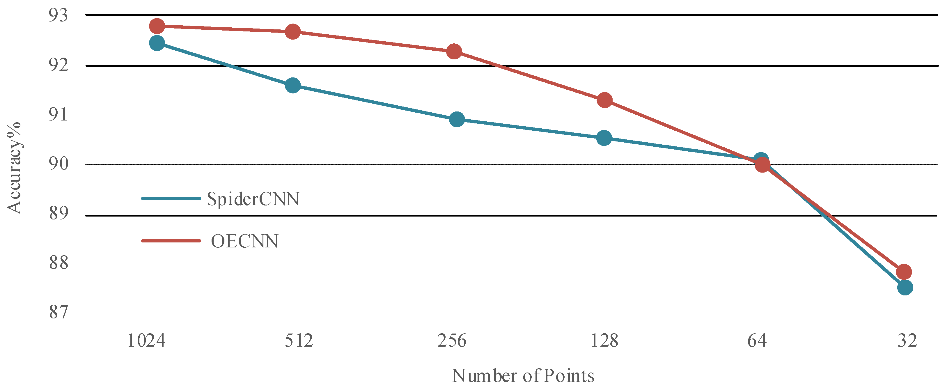
4.4. Robustness Test
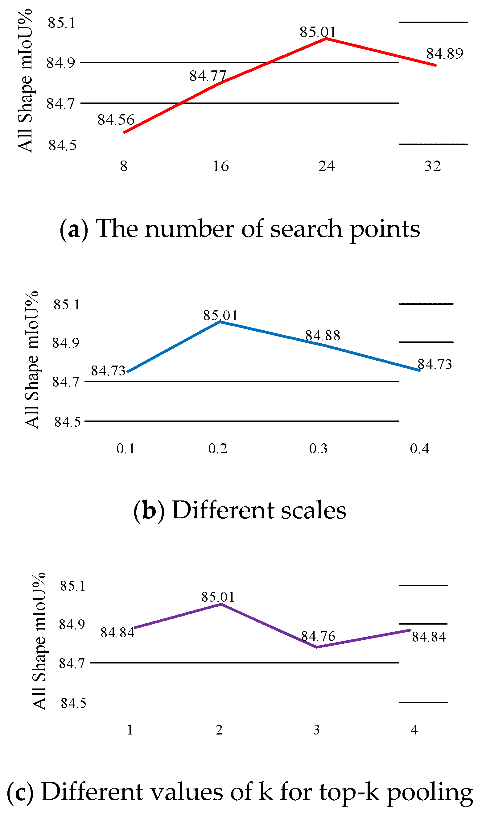
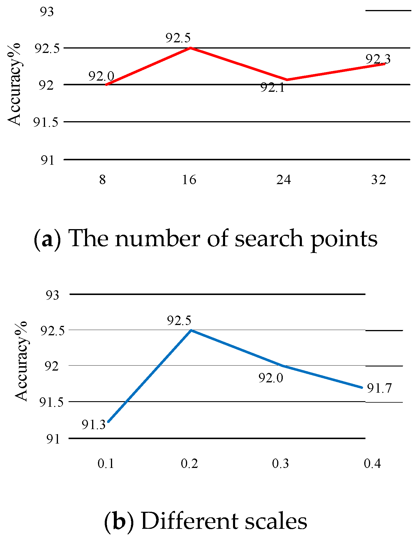
4.5. Ablation Experiments
4.6. Time and Space Complexity Analysis
5. Conclusions
Author Contributions
Funding
Institutional Review Board Statement
Informed Consent Statement
Data Availability Statement
Acknowledgments
Conflicts of Interest
References
- Krizhevsky, A.; Sutskever, I.; Hinton, G.E. ImageNet classification with deep convolutional neural networks. Commun. ACM 2017, 60, 84–90. [Google Scholar] [CrossRef]
- Szegedy, C.; Liu, W.; Jia, Y.Q.; Sermanet, P.; Reed, S.; Aanguelov, D.; Erhan, D.; Vanhoucke, V.; Rabinovich, A. Going deeper with convolutions. In Proceedings of the IEEE Conference on Computer Vision and Pattern Recognition (CVPR), Boston, MA, USA, 7–12 June 2015; pp. 1–9. [Google Scholar]
- Huang, G.; Liu, Z.; Maaten, L.V.D.; Weinberger, K.Q. Densely Connected Convolutional Network. In Proceedings of the 2017 IEEE Conference on Computer Vision and Pattern Recognition (CVPR), Honolulu, HI, USA, 21–26 July 2017; pp. 2261–2269. [Google Scholar]
- Long, J.; Shelhamer, E.; Darrell, T. Fully convolutional networks for semantic segmentation. In Proceedings of the 2015 IEEE Conference on Computer Vision and Pattern Recognition (CVPR), Boston, MA, USA, 7–12 June 2015; pp. 3431–3440. [Google Scholar]
- Chen, L.C.; Papandreou, G.; Kokkinos, L.; Murphy, K.; Yuille, A.L. DeepLab: Semantic Image Segmentation with Deep Convolutional Nets, Atrous Convolution, Fully Connected CRFs. IEEE Trans. Pattern Anal. Mach. Intell. 2017, 40, 834–848. [Google Scholar] [CrossRef] [PubMed]
- Wu, Z.; Song, S.; Khosla, A.; Yu, F.; Zhang, L.G.; Tang, X.; Xiao, J.X. 3D ShapeNets: A deep representation for volumetric shapes. In Proceedings of the 2015 IEEE Conference on Computer Vision and Pattern Recognition (CVPR), Boston, MA, USA, 7–12 June 2015; pp. 1912–1920. [Google Scholar]
- Maturana, D.; Scherer, S. VoxNet: A 3D Convolutional Neural Network for real-time object recognition. In Proceedings of the 2015 IEEE/RSJ International Conference on Intelligent Robots and Systems (IROS), Hamburg, Germany, 28 September–2 October 2015; pp. 922–928. [Google Scholar]
- Qi, C.R.; Su, H.; Niessner, M.; Dai, A.; Yan, M.; Guibas, L.J. Volumetric and Multi-View CNNs for Object Classification on 3D Data. In Proceedings of the 2016 IEEE Conference on Computer Vision and Pattern Recogniton (CVPR), Las Vegas, NV, USA, 27–30 June 2016; pp. 5648–5656. [Google Scholar]
- Riegler, C.; Ulusoy, A.O.; Geiger, A. OctNet: Learning Deep 4D Representations at High Resolutions. In Proceedings of the 2017 IEEE Conference on Computer Vision and Pattern Recognition (CVPR), Honolulu, HI, USA, 21–26 July 2017; pp. 6620–6629. [Google Scholar]
- Tatarchenko, M.; Dosovitskiy, A.; Brox, T. Octree Generating Networks: Efficient Convolutional Architectures for High-resolution 3D Outputs. In Proceedings of the IEEE International Conference on Computer Vision, Venice, Italy, 22–29 October 2017; pp. 2107–2115. [Google Scholar] [CrossRef] [Green Version]
- Qi, C.R.; Su, H.; Kaichun, M.; Guibas, L.J. PointNet: Deep Learning on Point Sets for 3D Classification and Segmentation. In Proceedings of the 2017 IEEE Conference on Computer Vision and Pattern Recognition, Honolulu, HI, USA, 21–26 July 2017; pp. 77–85. [Google Scholar]
- Qi, C.R.; Yi, L.; Su, H.; Guibas, L.J. PointNet++: Deep Hierarchical Feature Learning on Point Sets in a Metric Space. In Proceedings of the Neural Information Processing Systems (NIPS), Long Beach, CA, USA, 4–9 December 2017; pp. 5099–5108. [Google Scholar]
- Wang, C.; Samari, B.; Siddiqi, K. Local Spectral Graph Convolution for Point Set Feature Learning. In Proceedings of the European Conference on Computer Vision, Munich, Germany, 8–14 September 2018; pp. 56–71. [Google Scholar] [CrossRef] [Green Version]
- Xu, Y.; Fan, T.; Xu, M.; Zeng, L.; Qiao, Y. SpiderCNN: Deep Learning on Point Sets with Parameterized Convolutional Filters. In Proceedings of the European Conference on Computer Vision, Munich, Germany, 8–14 September 2018; pp. 90–105. [Google Scholar] [CrossRef] [Green Version]
- Wang, C.; Cheng, M.; Sohel, F.; Bennamoun, M.; Li, J. NormalNet: A voxel-based CNN for 3D object classification and retrieval. Neurocomputing 2019, 323, 139–147. [Google Scholar] [CrossRef]
- Graham, B.; Engelcke, M.; Van Der Maaten, L. 3D Semantic Segmentation with Submanifold Sparse Convolutional Networks. In Proceedings of the IEEE Conference on Computer Vision and Pattern Recognition (CVPR), Salt Lake City, UT, USA, 18–22 June 2018; pp. 9224–9232. [Google Scholar] [CrossRef] [Green Version]
- Masci, J.; Boscaini, D.; Bronstein, M.M.; Vandergheynst, P. Geodesic Convolutional Neural Networks on Riemannian Manifolds. In Proceedings of the 2015 IEEE International Conference on Computer Vision Workshop (ICCVW), Santiago, Chile, 7–13 December 2015; pp. 832–840. [Google Scholar]
- Jiang, M.Y.; Wu, Y.; Zhao, T.; Zhao, Z.; Lu, C.W. PointSIFT: A SIFT-like Network Module for 3D Point Cloud Semantic Segmentation. arXiv 2018, arXiv:1807.00652. Available online: https://arxiv.org/abs/1807.00652 (accessed on 28 July 2021).
- Chang, A.X.; Funkhouser, T.; Guibas, L.; Hanrahan, P.; Huang, Q.X.; Li, Z.M.; Savarese, S.; Savva, M.; Song, S.; Su, H.; et al. ShapeNet: An Information-Rich 3D Model Repository. arXiv 2015, arXiv:1512.03012. Available online: https://arxiv.org/abs/1512.03012 (accessed on 28 July 2021).
- Zaheer, M.; Kottur, S.; Ravanbakhsh, S.; Poczos, B.; Salakhutdinov, R.R.; Smola, A.J. Deep Sets. arXiv 2017, arXiv:1703.06114v3. Available online: https://arxiv.org/abs/1703.06114v3 (accessed on 28 July 2021).
- Klokov, R.; Lempitsky, V. Escape from Cells: Deep Kd-Networks for the Recognition of 3D Point Cloud Models. In Proceedings of the 2017 IEEE International Conference on Computer Vision (ICCV), Venice, Italy, 22–29 October 2017; pp. 863–872. [Google Scholar] [CrossRef] [Green Version]
- Hua, B.; Tran, M.; Yeung, S. Pointwise Convolutional Neural Networks. In Proceedings of the IEEE Conference on Computer Vision and Pattern Recognition (CVPR), Salt Lake City, UT, USA, 18–22 June 2018; pp. 984–993. [Google Scholar]
- Le, T.; Duan, Y. PointGrid: A Deep Network for 3D Shape Understanding. In Proceedings of the IEEE Conference on Computer Vision and Pattern Recognition (CVPR), Salt Lake City, UT, USA, 18–22 June 2018; pp. 9204–9214. [Google Scholar]
- Li, Y.Y.; Bu, R.; Sun, M.C.; Wu, W.; Di, X.H.; Chen, B.Q. PointCNN: Convolution On X-Transformed Points. Adv. Neural Inf. Process. Syst. 2018, 31, 828–838. [Google Scholar]
- Wang, Y.; Sun, Y.B.; Liu, Z.W.; Sarma, S.E.; Bronstein, M.M.; Wang, Y.; Sun, Y.; Liu, Z.; Sarma, S.E.; Bronstein, M.M.; et al. Dynamic Graph CNN for Learning on Point Clouds. ACM Trans. Graph. 2019, 38, 1–12. [Google Scholar] [CrossRef] [Green Version]
- Yi, L.; Su, H.; Guo, X.W.; Guibas, L. SyncSpecCNN: Synchronized Spectral CNN for 3D Shape Segmentation. In Proceedings of the 2017 IEEE Conference on Computer Vision and Pattern Recognition (CVPR), Honolulu, HI, USA, 21–26 July 2017; pp. 6584–6592. [Google Scholar]


| Method | Points | Accuracy (%) |
|---|---|---|
| PointNet [11] | 1024 | 89.2 |
| PointNet++ [12] | 5000 | 91.9 |
| SpecGCN [13] | 2048 | 92.1 |
| SpiderCNN [14] | 1024 | 92.4 |
| PointSIFT+OECNN [18] | 1024 | 90.3 |
| DeepSets [20] | 5000 | 90.0 |
| Kd-Network [21] | 1024 | 90.6 |
| Pointwise CNN [22] | 1024 | 86.1 |
| PointGrid [23] | 1024 | 92.0 |
| PointCNN [24] | 1024 | 92.2 |
| DGCNN [25] | 1024 | 92.2 |
| OECNN | 1024 | 92.7 |
| PointNet [11] | PointNet++ [12] | SSCN [26] | SpiderCNN [14] | PointSIFT+ OECNN [18] | OECNN | |
|---|---|---|---|---|---|---|
| aero | 83.4 | 82.4 | 81.6 | 83.5 | 83.3 | 83.1 |
| bag | 78.7 | 79.0 | 81.7 | 81.0 | 79.9 | 79.6 |
| cap | 82.5 | 87.7 | 81.9 | 87.2 | 85.8 | 89.6 |
| car | 74.9 | 77.3 | 75.2 | 77.5 | 77.3 | 79.1 |
| chair | 89.6 | 90.8 | 90.2 | 90.7 | 90.2 | 90.8 |
| ear phone | 73.0 | 71.8 | 74.9 | 76.8 | 77.1 | 78.9 |
| guitar | 91.5 | 91.0 | 93.0 | 91.1 | 90.9 | 91.6 |
| knife | 85.9 | 85.9 | 86.1 | 87.3 | 87.2 | 87.5 |
| lamp | 80.8 | 83.7 | 84.7 | 83.3 | 82.7 | 83.7 |
| laptop | 95.3 | 95.3 | 95.6 | 95.8 | 95.6 | 96.0 |
| motor | 65.2 | 71.6 | 66.7 | 70.2 | 71.3 | 73.0 |
| mug | 93.0 | 94.1 | 92. | 93.5 | 94.0 | 95.3 |
| pistol | 81.2 | 81.3 | 81.6 | 82.7 | 82.4 | 81.8 |
| rocket board | 57.9 | 58.7 | 60.6 | 59.7 | 59.6 | 62.7 |
| skate | 72.8 | 76.4 | 82.9 | 75.8 | 75.3 | 76.3 |
| table | 80.6 | 82.6 | 82.1 | 82.8 | 82.2 | 83.0 |
| mIoU | 83.7 | 85.1 | 84.7 | 85.3 | 84.9 | 85.5 |
| Classification (Accuracy) | Segmentation (mIoU) | |
|---|---|---|
| OEConv (filled by ) | 91.5% | 84.5% |
| OEConv (random) | 92.7% | 85.5% |
Publisher’s Note: MDPI stays neutral with regard to jurisdictional claims in published maps and institutional affiliations. |
© 2021 by the authors. Licensee MDPI, Basel, Switzerland. This article is an open access article distributed under the terms and conditions of the Creative Commons Attribution (CC BY) license (https://creativecommons.org/licenses/by/4.0/).
Share and Cite
Lin, H.; Zheng, W.; Peng, X. Orientation-Encoding CNN for Point Cloud Classification and Segmentation. Mach. Learn. Knowl. Extr. 2021, 3, 601-614. https://doi.org/10.3390/make3030031
Lin H, Zheng W, Peng X. Orientation-Encoding CNN for Point Cloud Classification and Segmentation. Machine Learning and Knowledge Extraction. 2021; 3(3):601-614. https://doi.org/10.3390/make3030031
Chicago/Turabian StyleLin, Hongbin, Wu Zheng, and Xiuping Peng. 2021. "Orientation-Encoding CNN for Point Cloud Classification and Segmentation" Machine Learning and Knowledge Extraction 3, no. 3: 601-614. https://doi.org/10.3390/make3030031
APA StyleLin, H., Zheng, W., & Peng, X. (2021). Orientation-Encoding CNN for Point Cloud Classification and Segmentation. Machine Learning and Knowledge Extraction, 3(3), 601-614. https://doi.org/10.3390/make3030031