1. Introduction
The ability to predict possible future actions of traffic participants is essential for anticipatory driving. As a human driver, we can make safe decisions in traffic because we automatically anticipate events based on our experience. In autonomous driving scenarios, predictions of probable future events can prove beneficial when used as additional inputs to the system. They can help to plan the next action more efficiently and to make decisions more informedly.
One way of realizing this is to extract information from an automatically rendered future frame. However, to extract information that can reliably support an autonomous driving system, the predicted frames have to be of high and stable visual quality. Therefore, the underlying video prediction network must constantly produce high-quality predictions, independent of variations in the input observations. Because of the domain shift between datasets, this is hard to achieve in reality. Yu et al. [
1], for example, demonstrated that problem when they tested a semantic segmentation network that was trained on the Cityscapes [
2] training subset. It achieved good results on the Cityscapes test subset, but poor results on the BDD100K [
1] test subset. One solution to reduce the effects caused by the domain shift between the training examples and the test data is to enforce the prediction network to learn generic representations of the appearance and motion of objects. An advantage of generic features is that they can quickly be fine-tuned to new scene contents or tasks when used to initialize another network. The learned features of an ideal network for video prediction match both of the following criteria. First, they are generic enough to enable the model to generalize well over a variety of different scene contents. Secondly, they produce high-quality predictions that preserve details of the observed input scene across multiple prediction steps.
Simple prediction models are already capable of producing next frames of sufficient quality, while still being lightweight and requiring little training time. However, these models often fail for new datasets, and their long-term predictions are generally blurry. In this paper, the focus lies on investigating to what extent it is possible to have both the advantages of such a lightweight model and a good generalization performance. The idea is to find a loss function that enforces the model to learn features that meet the criteria described earlier. Our model is a three-layer convolutional long-short term memory (ConvLSTM) [
3] network, which predicts the next frame based on four past frames. We train the network using 21 different combinations of seven loss terms. The loss terms range from terms that perform a pixel- or feature-based comparison to adversarial terms. To properly assess their generalization abilities, we evaluate all models on four datasets of increasing visual distance to the training data.
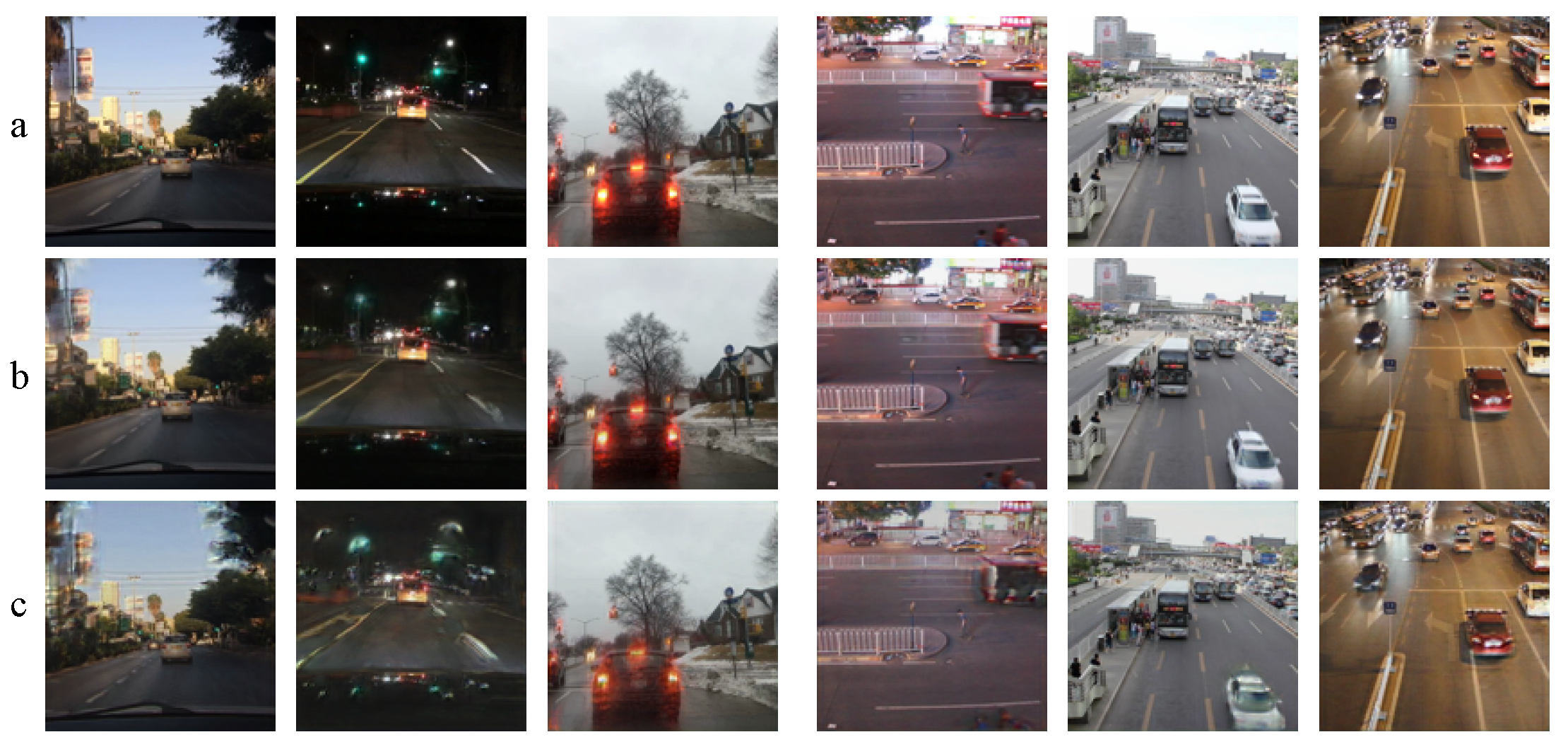
Figure 1 shows exemplary next frame predictions for two of these datasets. Further, we generate frames up to 20 time-steps ahead to evaluate the long-term prediction performance of the models. To quantify the model performance, we calculate traditional pixel-based evaluation metrics, as well as more advanced feature-based ones.
Our main contribution is the in-depth evaluation of the generalization abilities of a deep learning-based next frame video prediction network. In particular, this work provides detailed analyses of how different loss combinations influence the prediction quality. Based on these analyses, we can draw informed conclusions about the learned representations of the network. Our experiments show that an intelligently designed loss function is crucial as, it helps to stabilize the visual quality of the predictions over a variety of datasets and to improve the training convergence. The best performing loss combination can boost the prediction performance by 55% for the next frame predictions, and by 50% for the 10th frame predictions, in comparison to other loss combinations.
2. Related Work
The application of deep learning-based video prediction models for traffic scenes has become a popular field of research, in the last years. After Ranzato et al. [
5] first introduced a general baseline for deep learning-based video prediction in 2014, many approaches explicitly started to focus on predicting traffic scenes.
The recurrent neural network [
6,
7,
8,
9,
10,
11,
12,
13] is a widely used network architecture in such models. Similar to our approach, Lotter et al. [
7], for example, generate the pixel values of the frame one time-step ahead using long short-term memory (LSTM) [
14] units.
Although a lot of effort has been put on this topic, generating plausible predictions of high visual quality over a variety of datasets is still not solved, especially not for real-world scenarios. The predictions often lack realism, particularly for distant future frames. The main problem of the video prediction task is: the future is uncertain and the nature of the model output is multi-modal.
One approach to tackle this is to directly address the uncertainty of the prediction output. Bhattacharyya et al. [
15], for instance, recently proposed a novel Bayesian formulation, that jointly captures the model and the observation uncertainty to anticipate future scene states. Another way to address the uncertainty is to use a generative adversarial network (GAN) [
16] as a framework for training [
17,
18,
19,
20,
21].
A second approach to handle the problem of implausible prediction outputs that lack realism is to reduce the complexity of the problem. Many authors, for example, used data with lower-dimensional image content, such as label images, instead of natural image scenes [
12,
15,
22,
23,
24,
25]. Others split the problem into two problems, motion and content prediction, and learn separate representations for the static and dynamic components. For training, these approaches either use a motion prior, such as optical flow information [
9,
20,
23,
26,
27,
28], as a conditional input or use learned features to represent pixel dynamics [
29].
Our approach builds on the idea of utilizing the loss function to enforce the network to learn feature representations that are more generic and less influenced by dataset-specific content. A loss term that helps the network to map motion to learned object representations rather than solely to individual pixel values could lead to a more realistic foreground and background separation. In this paper, we evaluate the influence of different loss terms on the generalization abilities of a prediction model. For traffic prediction models, it is common to train models on the KITTI [
30] dataset and test them on the Caltech Pedestrian [
31] dataset, or vice-versa [
20,
29]. However, the domain shift between these datasets is comparatively small. To our knowledge, Luc et al. [
22] are the only other authors who directly investigate the generalization abilities of their traffic scene prediction model. There are detailed ablation studies of other authors that focus on the influence of the model complexity [
11] or the loss functions [
19], but they only measure the in-domain performance of the models.
3. Methodology for Predicting the Next Frame of Traffic Scenes
We follow a purely data-driven approach to predict the next frame of traffic scenes, assuming that additional input information or costly ground truth labels are not always available. Our approach incorporates a generative model to assist in the development of model-inherent attention mechanisms. This generative model, the prediction network, is based on a ConvLSTM architecture that is commonly used in similar forms as a baseline network [
6,
7,
13], which makes our results easy to transfer. Its convolution operations function as a spatial and its LSTM units as a temporal attention mechanism. During training, the model optimizes the 3726019 parameters of the prediction network by minimizing the loss function. Our loss functions contain different combinations of non-adversarial and adversarial loss terms. The non-adversarial loss terms are trained in a supervised setting by directly comparing the ground truth frame and the predicted frame. The adversarial loss terms are trained in a self-supervised setting, where a second network, the discriminator network, is used [
16]. To efficiently demonstrate the influence of each loss term, we built on low-level processing without costly upstream mechanisms. Following, we describe the technical details of the next frame prediction model and the different loss terms.
3.1. Next Frame Prediction Model
3.1.1. Prediction Network
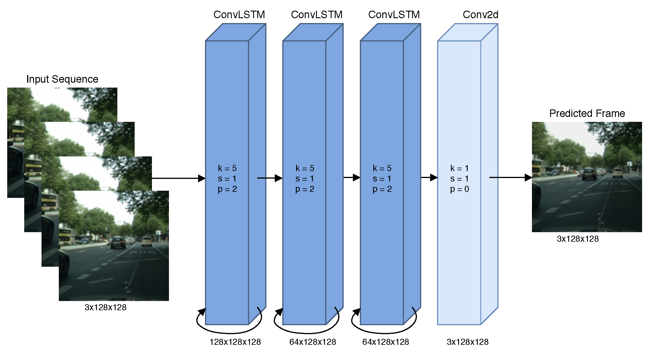
The resolution preserving three-layer ConvLSTM [
3] network
G, illustrated in
Figure 2, is the core network that generates the predictions. It sequentially processes the frames of an input sequence
and transforms them into the next future frame
of the sequence. The parameter
corresponds to the temporal depth of the input sequence. We use three ConvLSTM layers with convolutional kernels of size
, a stride of 1, zero-padding of 2, and feature sizes of 128, 64, and 64. Additionally, we use one 2d convolutional layer with a kernel size of
, stride 1, and zero-padding of 0, to map from feature-space to RGB-space.
3.1.2. Discriminator Network
When using an adversarial loss term to train the prediction model we utilize a second network, the discriminator network
D. For
D, we adopt the structure of the discriminator network of Aigner and Körner [
18] for resolutions of
, without progressive growing. As an input,
D alternately receives
frames from the training set, representing the ground truth sequence, and
. The latter sequence consists of the input and output frames of
G.
D outputs a score
or
, respectively. This score ranks the given input as either being real or fake. The labels for real sequences are set to
and the labels for fake sequences to
. We use weight scaling in
G and in
D to stabilize the training, as originally proposed by Karras et al. [
32].
3.2. Loss Terms
The following paragraphs describe the individual terms of our training losses briefly. When combining different loss terms in one loss function, we multiplied each loss term by a loss-specific weight factor . For simplicity, we refer to the ground truth frame as x and the predicted frame as .
3.2.1. L1 Loss
This loss measures the mean absolute error (MAE) between the elements of the ground truth and the predicted frame. It is defined as
where
n and
m are the width and height of the frames.
3.2.2. L2 Loss
The L2 loss measures the mean squared error (MSE) between each element of the ground truth and the predicted frame. It is defined as
3.2.3. BCE Loss
This loss measures the binary cross-entropy (BCE) between the ground truth and the predicted frame. It is defined as
where
x takes its values in
and
in
.
3.2.4. Perceptual Loss
The perceptual loss [
33] measures the L2 difference between the feature maps of the ground truth and the predicted frame of a specific layer from the VGG-19 [
34] network, pre-trained on ImageNet [
35]. Contrary to the L1 and L2 losses, which directly measure the image differences in pixel-space, the perceptual loss measures the differences in feature-space. It is defined as
where
is the feature map obtained before the
k-th max-pooling layer and after the
l-th convolutional layer of the pre-trained VGG-19 network.
and
are the width and height dimensions of the feature maps.
3.2.5. GDL Loss
The image gradient difference loss (GDL) [
36] computes the differences between the image gradients of the ground truth and the predicted frame. The GDL loss is given by
where
.
3.2.6. GAN Loss
This loss term is the standard loss function of the GAN [
16]. It is based on the Jenson-Shannon-divergence between the distributions of the ground truth frames and the predicted frames. The loss function to train
D is
and the loss function to train
G is
3.2.7. WGAN-gp Loss with Epsilon Penalty
This loss consists of the Wasserstein GAN with gradient penalty (WGAN-gp) [
37] loss and an epsilon penalty [
32] term that prevents the loss from drifting. It is based on measuring the Wasserstein distance between the distributions of the ground truth frames and the predicted frames. The WGAN-gp loss with epsilon penalty for optimizing
D is defined as
As described by Gulrajani et al. [
37],
is the data distribution,
is the model distribution, implicitly defined by
,
,
is the epsilon-penalty coefficient, and
is the gradient-penalty coefficient.
is implicitly defined, sampling uniformly along straight lines between pairs of points sampled from the data distribution
and the
G distribution
. The WGAN-gp loss for optimizing
G is defined as
The penalty coefficients of the WGAN-gp loss with epsilon-penalty are
and
, as proposed by Karras et al. [
32].
4. Experiments and Evaluation
To analyze the influence of each loss term on the model performance, we conducted experiments on 5 different datasets and trained our model on 21 different loss combinations. The next subsections contain details about the training settings, the datasets, and the analyses of the quantitative and qualitative results.
4.1. Training Settings
We trained the model described in
Section 3.1 using the 21 losses listed in
Table 1. To weight the loss terms in a combined loss function, we set
and
. The other weight factors were set to 1. When combining the perceptual loss term solely with the GDL term, we set
and
. These values were heuristically chosen to balance the individual loss terms at a similar range. For the GDL loss, we set
, when combining it with an L1 term, and
, when combining it with an L2 loss term. To train the networks with adversarial loss terms, we applied weight scaling in
G and
D, as described by Karras et al. [
32]. All 21 different prediction models were trained to predict the next frame after receiving four past frames as an input. We trained each model on the full Cityscapes Sequences [
2] dataset with a batch size of 4 and a fixed random seed. As an optimization algorithm, we used the Adam optimizer [
38] with
and
. The initial learning rate was
. Every 10th epoch, we decayed the learning rate by a heuristically set factor of
. In total, all networks trained for 30 Epochs. Intermediate states were saved every 5th epoch for evaluation purposes. We trained the networks on an Asus GeForce RTX 2080 Ti GPU with 11
of RAM, except for most of the networks with a GAN loss term, which we trained on an NVIDIA Titan X Pascal with 12
of RAM. The code was implemented in PyTorch.
4.2. Datasets
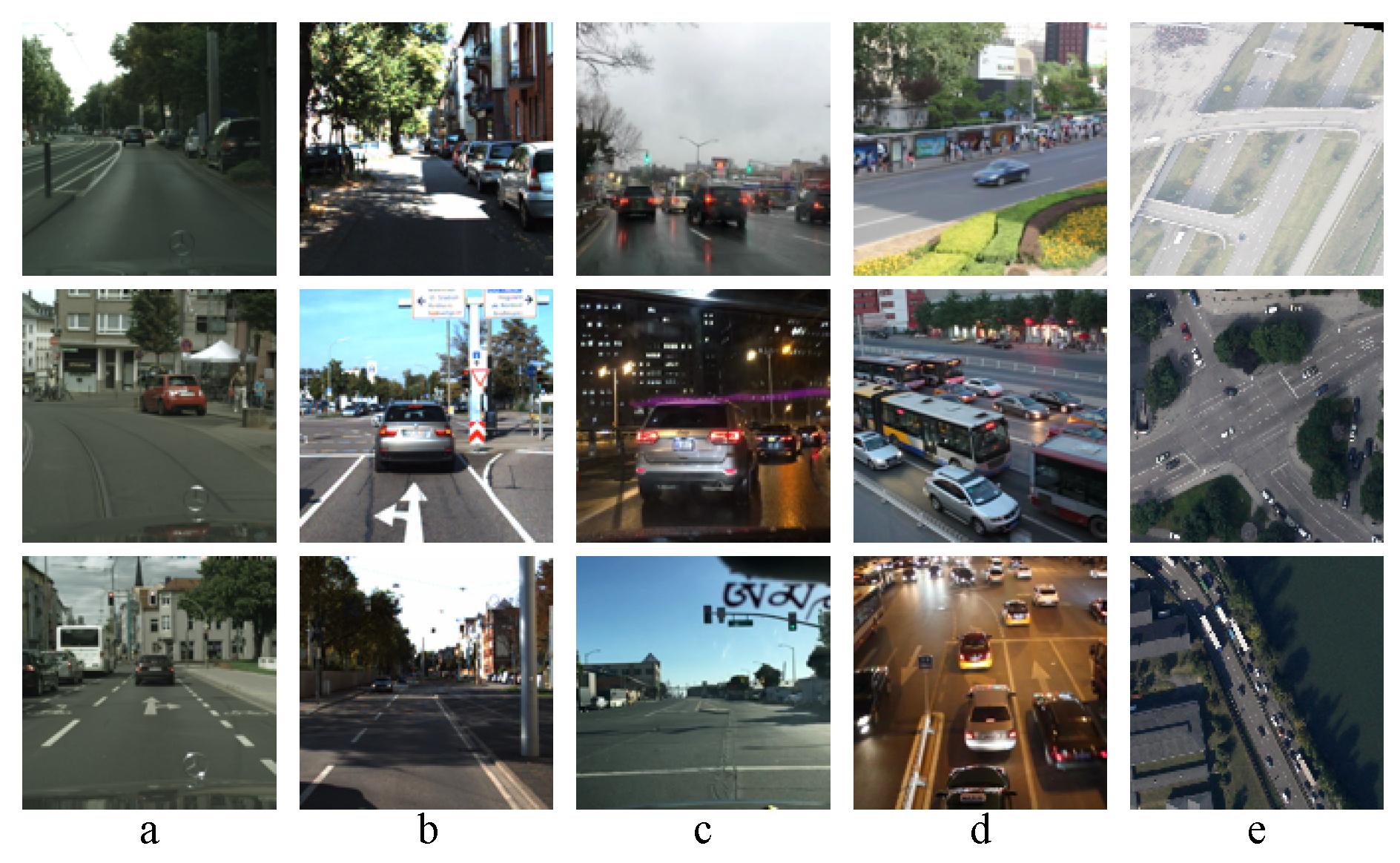
We conducted experiments on five different datasets. For training, we used the full Cityscapes Sequences [
2] dataset. For testing, we used four other datasets with an increasing domain shift to the training dataset—KITTI Tracking [
30], BDD100K [
1], UA-DETRAC [
4], and KIT AIS Vehicles [
39]. We chose these test datasets to investigate to what extent each model can generalize to new scenes. All frames for training and testing were retrieved by first center cropping and then resizing them bilinearly from their original resolution to a resolution of
.
Figure 3 shows example images from every dataset. The following paragraphs describe the datasets and the specifications of our customized subsets that we used to calculate and compare the evaluation metrics.
4.2.1. Cityscapes
The Cityscapes Sequences dataset consists of 5000 videos, that is, 2975 for training, 500 for validation, and 1525 for testing. These 8-bit color videos were recorded with a frame rate of 17 and an original resolution of in 50 different cities, primarily in Germany. The videos mainly show urban street scenes and a few different highway scenarios in similar weather and time conditions, that is, sunny, partly cloudy, and cloudy during daytime in spring, summer, and fall. All videos are 30 frames long. We used the full 5000 videos of the dataset for training. Since we trained our networks to predict the next frame based on four past frames, we had 30,000 training sequences in total.
4.2.2. Kitti Tracking
The KITTI Tracking sequences are recorded in Karlsruhe, Germany. The dataset contains 21 training and 29 testing videos, all of a varying sequence length and with an original resolution of
. The videos were captured at a frame rate of 10
, which results in higher motion differences in-between frames compared to our training examples. Otherwise, the displayed scenes are similar to those of Cityscapes but more evenly distributed between rural, urban street, and highway scenarios. The weather and time conditions match those of Cityscapes. For testing, we used the test split as provided by Geiger et al. [
30]. To calculate the evaluation metrics and for comparison with the other datasets, we built a subset of 100 sequences using 24 frame-long snippets that were evenly distributed across the test sequences.
4.2.3. Bdd100k
The complete BDD100K dataset consists of 100,000 videos with an original resolution of
. All videos are 40 seconds long and captured at 30
in either New York, Berkeley, San Francisco, or the Bay Area. The test subset of 20,000 videos, provided by Yu et al. [
1], contains 20 splits with 1000 videos each. For testing and evaluating, we took the first split of this test set. To roughly match the Cityscapes frame rate, we sub-sampled it to 15
. We then used the first 24 frames of every 10th sequence of the resulting split to build a customized test set of 100 sequences. The BDD100K videos were recorded under six different weather conditions, that is, clear, partly cloudy, overcast, rainy, snowy, and foggy, and during three different daytimes, that is, day, night, and dusk/dawn. This means the BDD100K scenes display completely different locations and a greater variety of weather and lighting conditions compared to the Cityscapes scenes.
4.2.4. Ua-Detrac
The full UA-DETRAC dataset consists of 100 videos, 60 for training, and 40 for testing, all of a varying sequence length and an original resolution of . The videos were captured at a frame rate of 25 at 24 different static locations in Beijing and Tianjin, China. The recorded scenes contain surveillance views of residential roads, highways, tunnels, gas stations, and a parking lot during day-time, night-time, and different weather conditions. As a result, the UA-DETRAC videos not only show different scene contents, compared to the training examples, but they also have different viewing angles and do not display any ego-motion. Additionally, the lower UA-DETRAC frame rate causes smaller differences in object motion in-between frames. To test and evaluate our models, we built a customized subset of 100 evenly distributed sequences of length 24 frames from the original test split.
4.2.5. KIT AIS Vehicles
The KIT AIS Vehicles dataset [
39] consists of a single training split, which contains 9 sequences of aerial images with varying sequence lengths. The videos display different highway, crossroads, and street scenarios. All sequences are of varying original frame resolutions, captured at 2
from varying heights above the ground during similar weather and time conditions. In comparison to Cityscapes, this is the most challenging dataset. The viewing angle, the object motions, and the scene contents differ completely. We used the whole dataset, as provided by Schmidt [
39], for testing. Due to insufficient sequence lengths, we predicted 10 future frames based on four input frames for this dataset. This resulted in a customized subset of 24 sequences for evaluation.
4.3. Evaluation Metrics
To quantitatively rate the performance of video prediction models, there is no consistent evaluation scheme. Traditionally, pixel value-based image comparison metrics, such as the mean squared error (MSE), the peak signal-to-noise ratio (PSNR), and the structural similarity index (SSIM) [
40] are used by most authors. Although these metrics are very common for comparing video prediction approaches, there is one big problem. The values of these metrics often do not correlate well with the human perception of visual image quality. To assess this problem, we calculate two, more recent, evaluation metrics, the Fréchet inception distance (FID) [
41], and the learned perceptual image patch similarity (LPIPS) [
42] in addition to the MSE, the PSNR, and the SSIM. These metrics have shown to better correlate with human judgments about visual image quality. In contrast to the traditional metrics, which directly compare the pixel values of two images, the FID and the LPIPS values measure the distance between two images not in pixel-space, but feature-space. Their values are obtained based on the feature activations of one or more layers of a second, pre-trained, neural network. To calculate the FID and LPIPS values, we followed the procedures described by Heusel et al. [
41] and Zhang et al. [
42]. For the FID metric, we used an InceptionV3 [
43] network, pre-trained on ImageNet [
35]. For the LPIPS metric, we used the pre-trained network provided by Zhang et al. [
42].
4.4. Qualitative and Quantitative Analyses
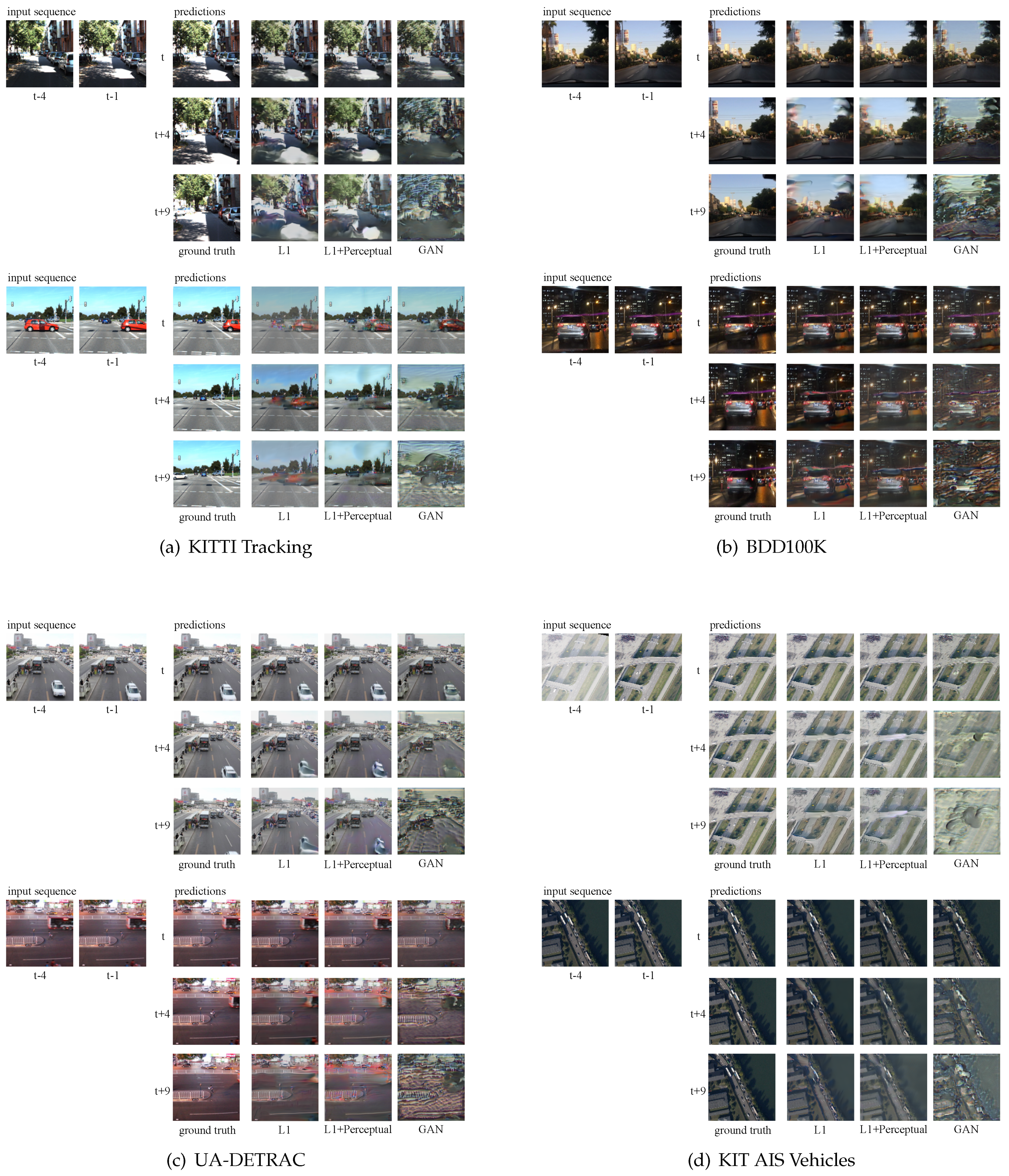
To properly assess the generalization abilities of a prediction model, it is important to evaluate its capability to generalize both to new datasets and a higher number of prediction steps. Therefore, we generated long-term predictions for four test datasets with every model. During testing, we let the models predict 20 future frames for the KITTI Tracking, the BDD100K, and the UA-DETRAC dataset and 10 future frames for the KIT AIS Vehicles dataset, because of insufficient sequence lengths in the dataset. To generate the long-term predictions, each predicted next frame of the model was recursively fed back in as an input. This means the long-term predictions during test time were based on only four real observations.
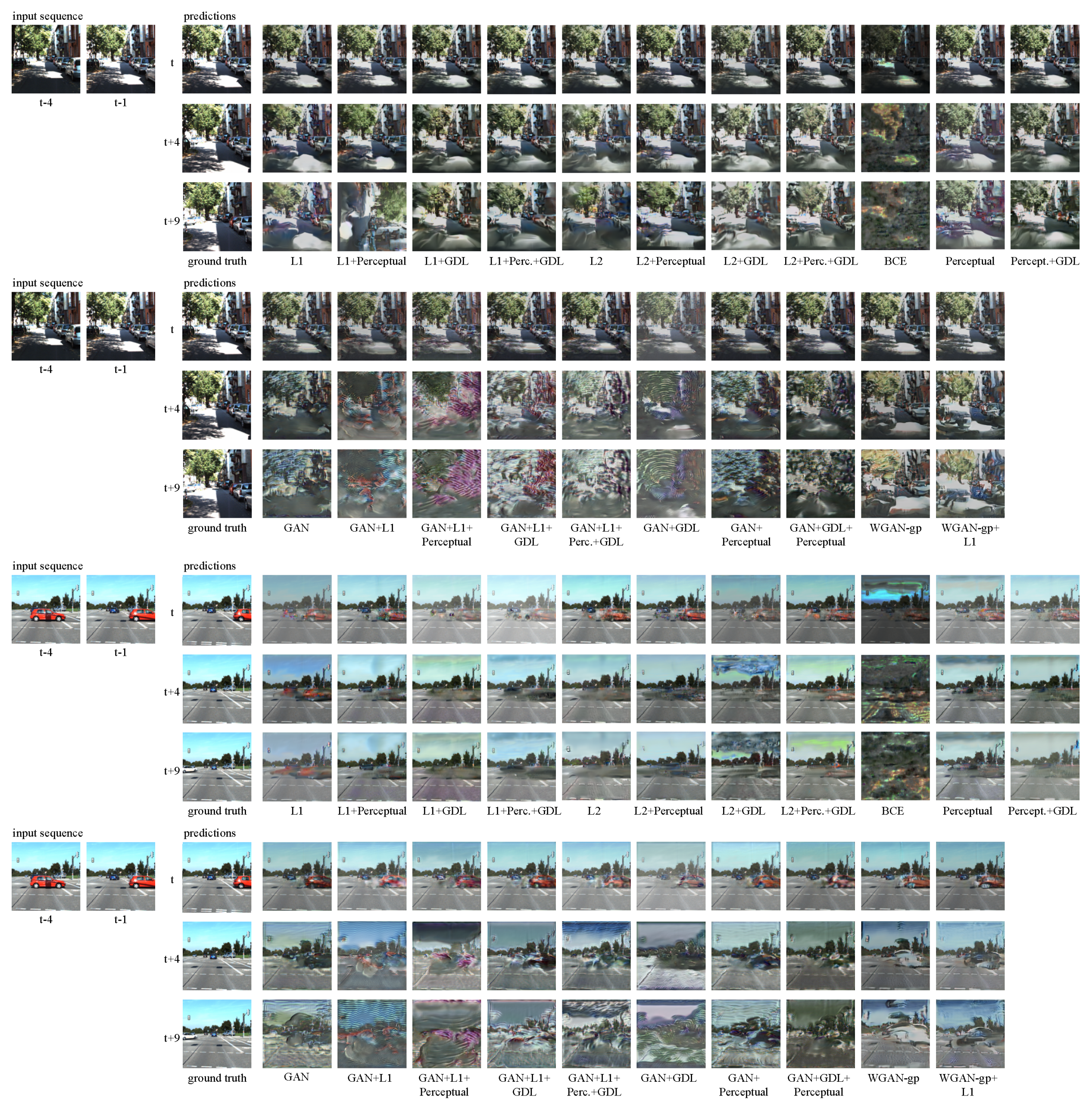
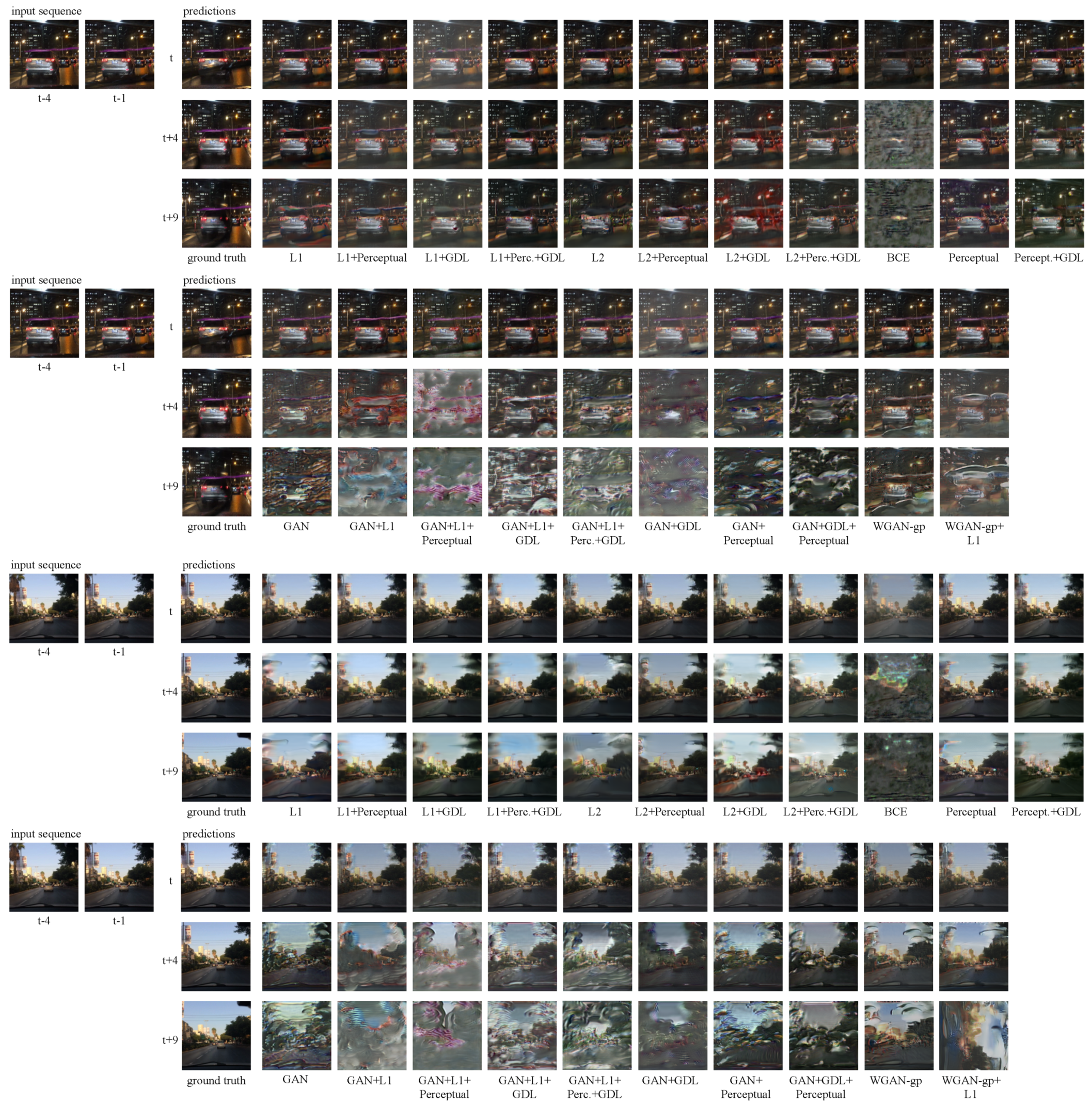
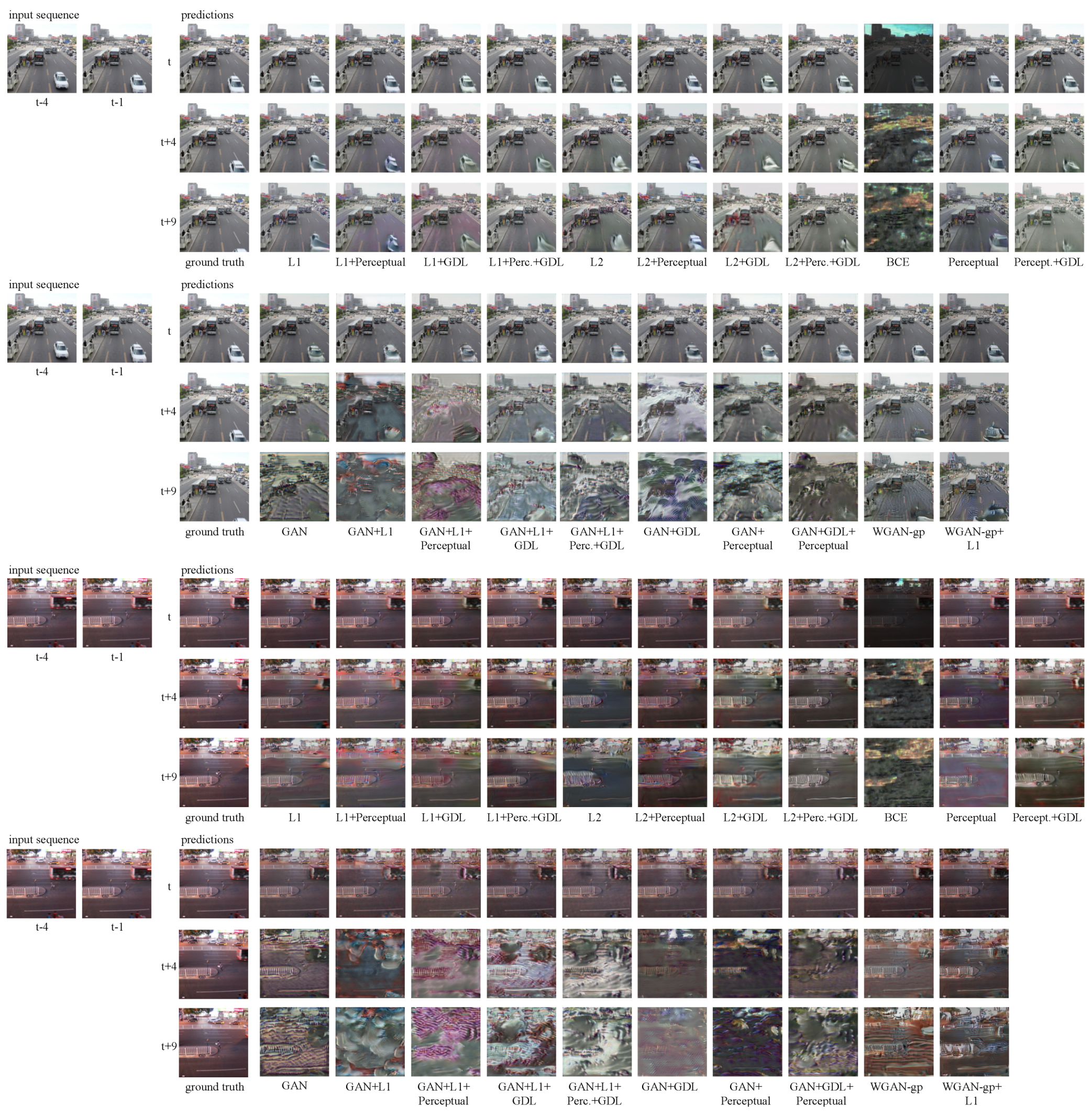
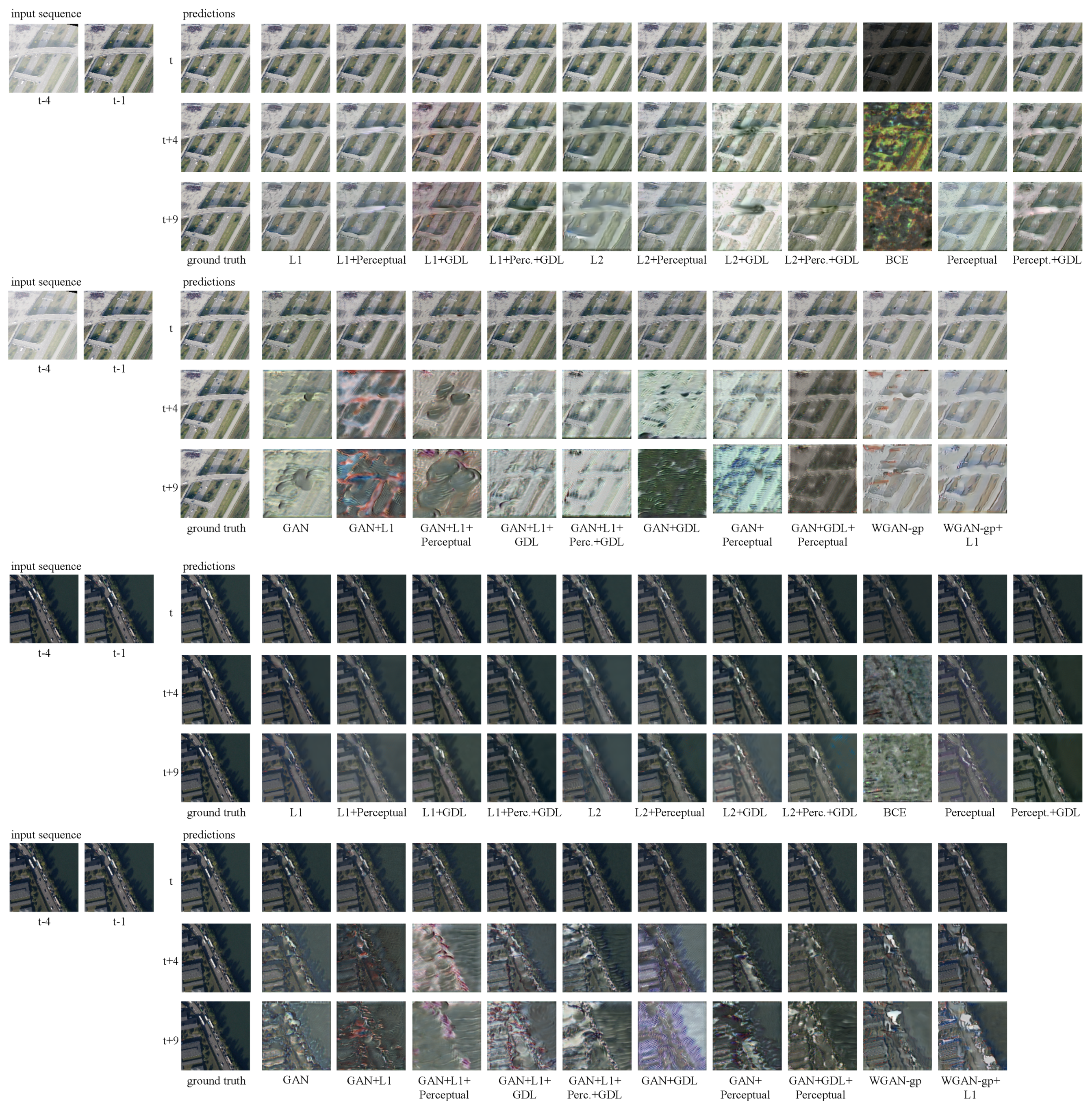
Figure 4 shows the qualitative results of these predictions by three selected models of different loss combinations for all four datasets. The qualitative results of all loss combinations can be found in
Appendix B. Additional videos and images are included in the
Supplementary Materials.
For the quantitative evaluation of the models, we calculated the metrics described in
Section 4.3. To calculate these quantitative measures, if not otherwise stated, we used our customized subsets, as described in
Section 4.2. They each contain 100 sequences of length 24 frames, except for KIT-AIS Vehicles, where only 24 sequences of length 14 frames were available.
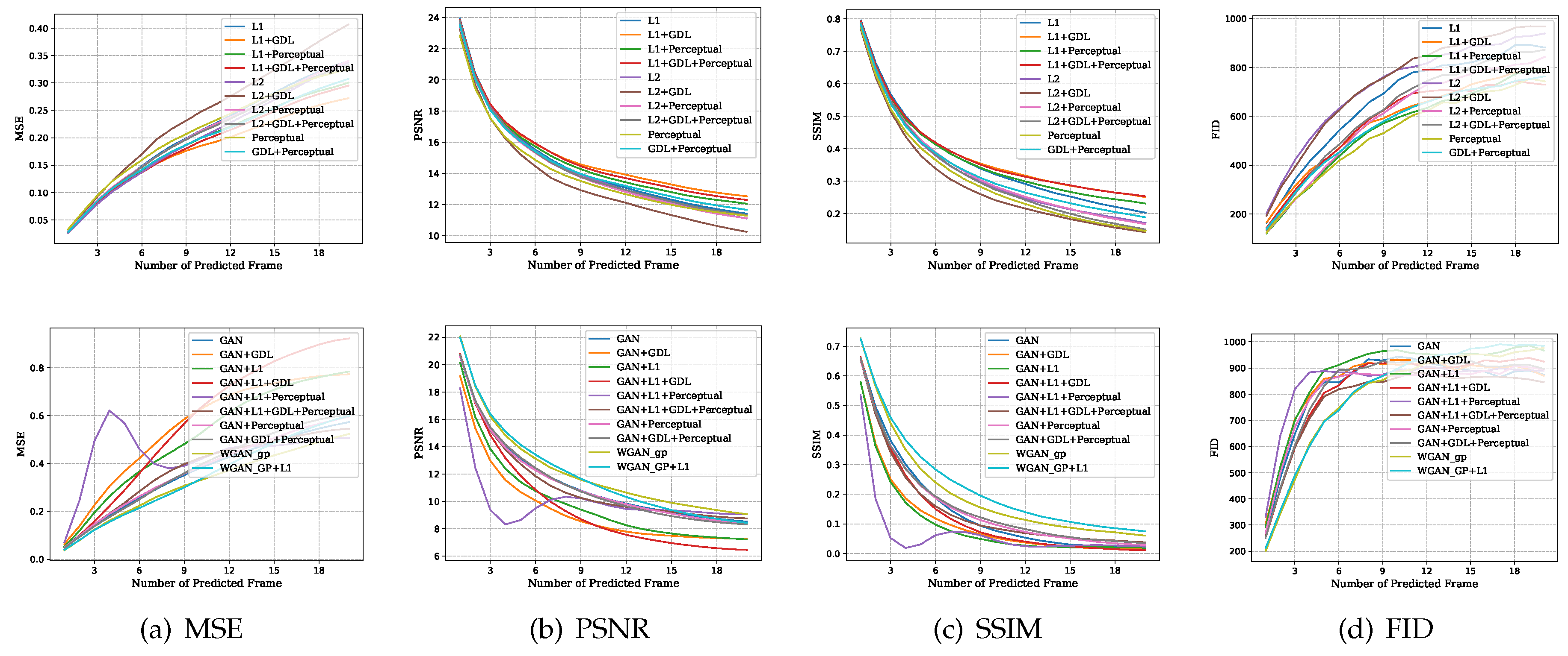
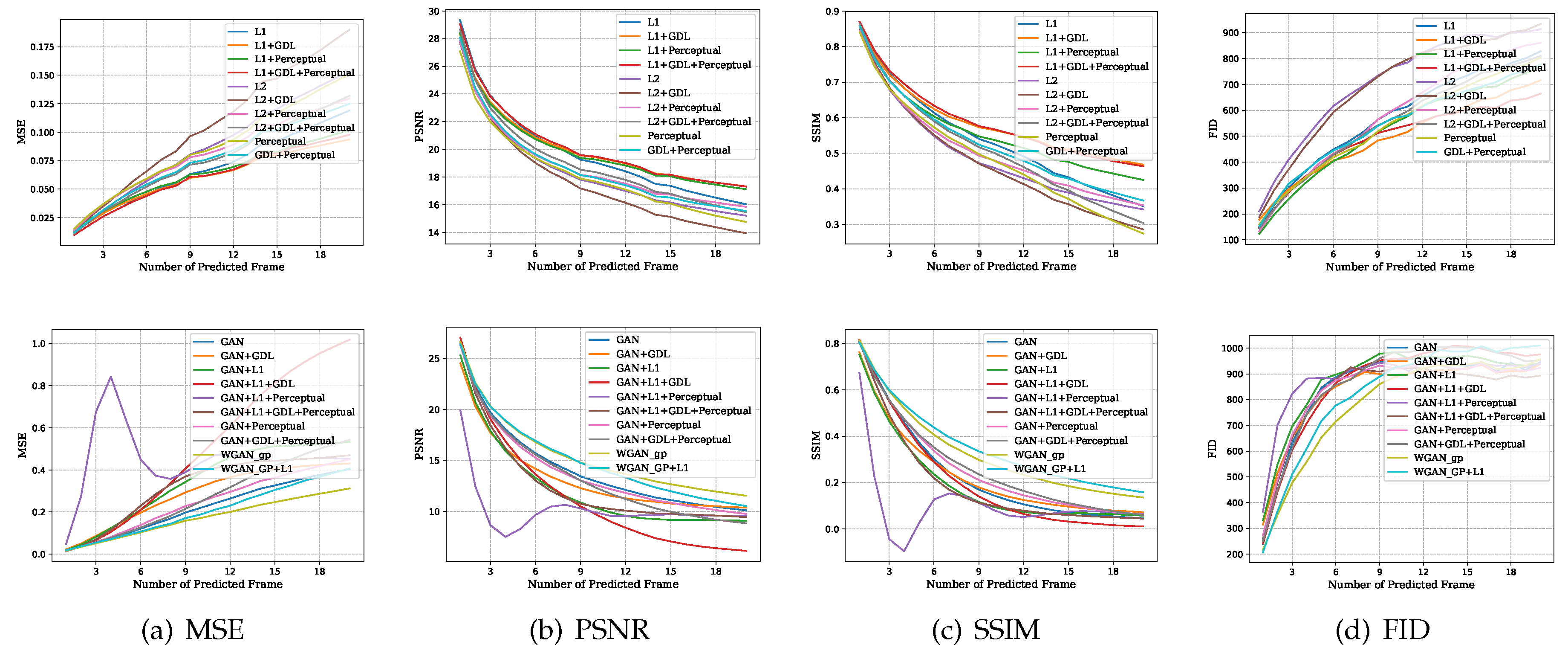
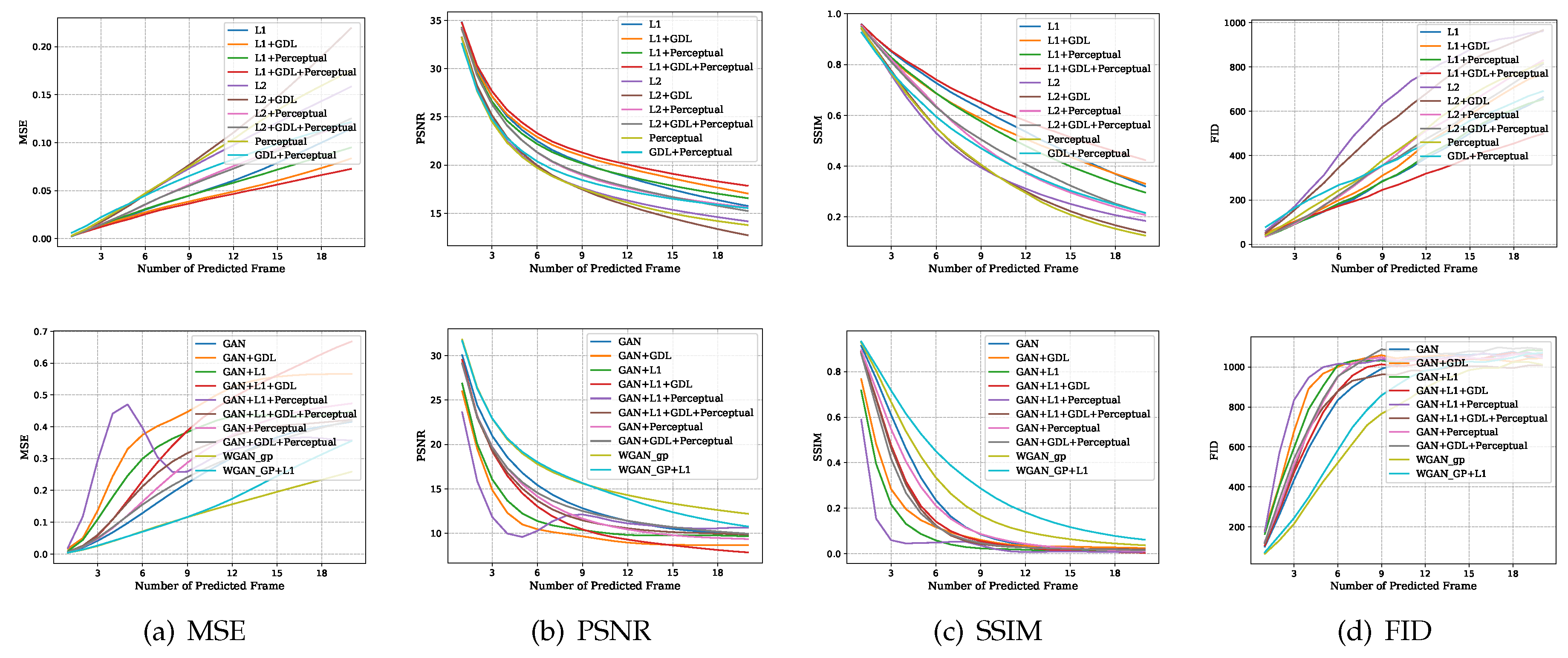
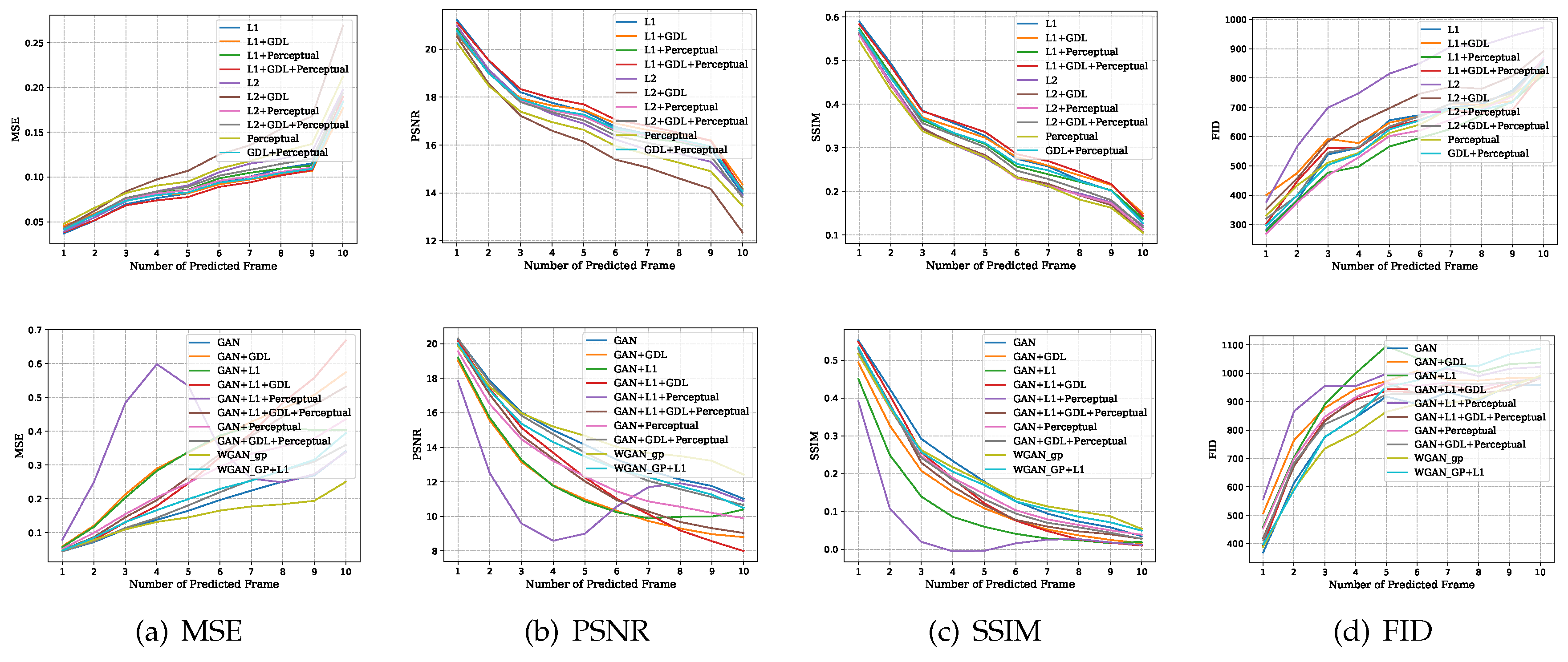
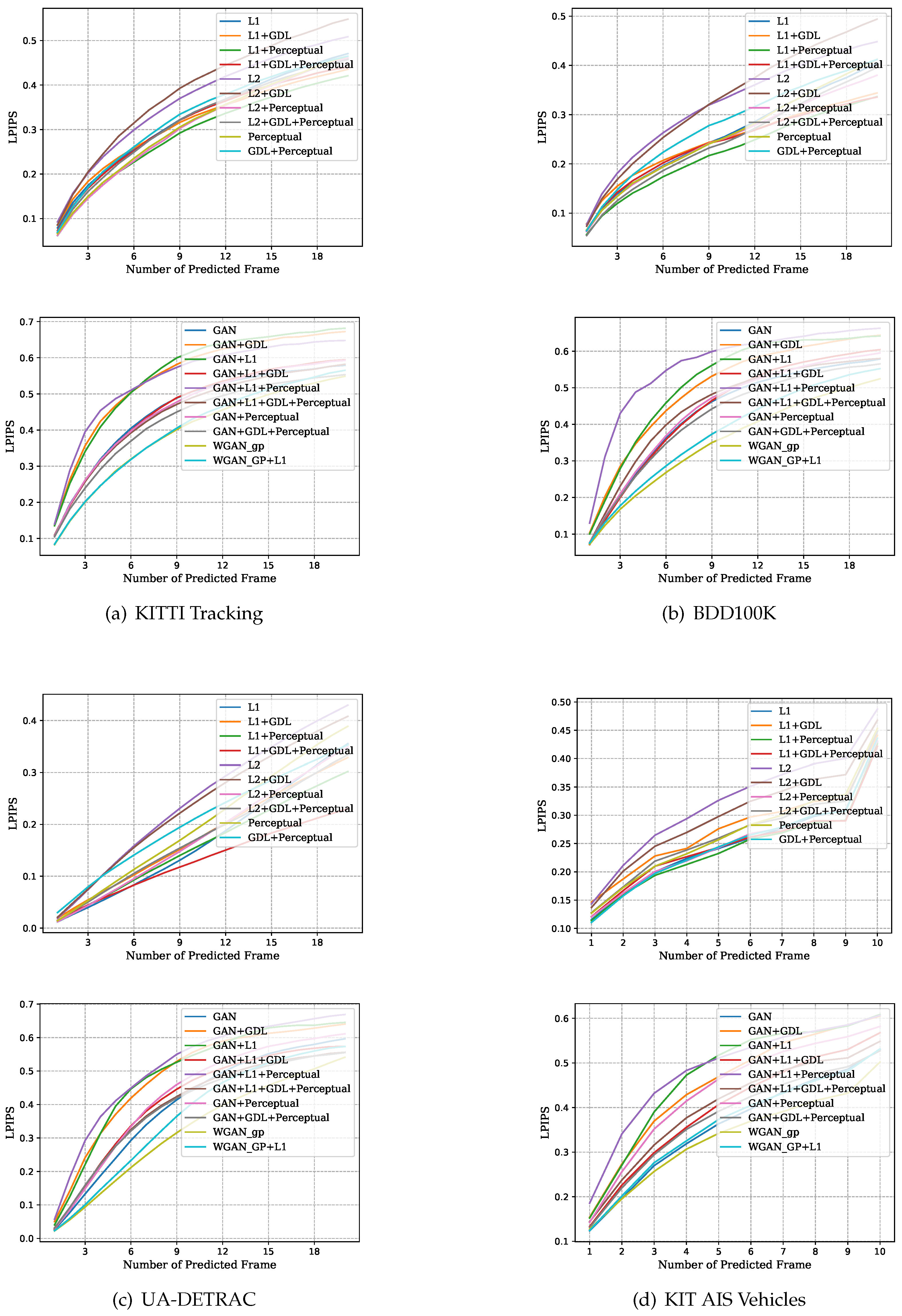
Figure 5 visualizes the LPIPS distance values per predicted frame for every model and dataset. This provides an overview of how the different loss combinations perform quantitatively in comparison. The visualizations of the MSE, PSNR, SSIM, and FID values are included in
Appendix A.
Table 2 lists the SSIM values for all models and all intermediate model states at every fifth training epoch exemplary for the KITTI Tracking dataset. This table gives an impression on how the different loss combinations influence the training convergence of the models.
5. Discussion and Conclusions
In this paper, we have shown that an intelligently designed loss function is essential for a prediction model to generate plausible next frames of traffic scenes. An optimal choice of the training loss leads to both good test performance and high generalization abilities of the model. We provided qualitative and quantitative evaluations on the influence of the individual loss terms. These evaluations strongly suggest that the combination of loss terms is particularly important for enabling the network to learn generic representations of object motion and appearance.
For our experiments, we used a ConvLSTM video prediction network that was trained on the Cityscapes dataset to predict the next frame after observing a sequence of four frames. In total, we trained 21 different combinations of seven individual loss terms. To draw informed conclusions about the generalization capabilities, we tested the resulting models on four different datasets of increasing visual distance to the training dataset. During testing, we generated long-term predictions for every dataset. After evaluating the predictions qualitatively, we could see great performance differences between the different loss combinations, especially when inspecting the long-term prediction results. The best performing model was the model that was trained on a combination of the perceptual and the L1 loss term. This model preserved object-specific features such as color and detailed content of the input scene across multiple prediction steps for all datasets. Models that were solely trained with a per-pixel error loss or an adversarial loss often averaged out such features, leading to a quick loss of detail after a few prediction steps. These predictions, therefore, tended to get blurry earlier. The predictions of the best performing model, on the other hand, remained sharp for a higher number of prediction steps. Additionally, the best performing model was able to identify moving objects and correctly propagate motion patterns across several time-steps. Interestingly, this was even the case for the KIT AIS Dataset, although it was recorded at a completely different frame rate and from a different viewing angle than the training data. For the quantitative evaluation of the models, we calculated three traditional pixel-based image comparison metrics, the MSE, the PSNR, and the SSIM. In addition to those metrics, we calculated two more advanced feature-based image comparison metrics, the FID, and the LPIPS. These feature-based evaluation metrics confirmed our visual impression of the qualitative results. The best performing loss combination generated next frame predictions up to 55% better and 10th frame predictions up to 50% better compared to the predictions of models trained with other loss combinations. These numbers were obtained from the LPIPS values.
Our experiments verify that an intelligent combination of loss terms is essential. It enables even a very lightweight model to reliably produce high-quality predictions over a variety of datasets. The evaluations suggest that the well-performing loss functions, in contrast to the other ones, helped the model to learn generic representations of the appearance and motion of objects and how to propagate these features correctly across time.
Author Contributions
Conceptualization, S.A. and M.K.; Methodology, S.A.; Software, S.A.; Validation, S.A. and M.K.; Formal analysis, S.A. and M.K.; Investigation, S.A.; Resources, M.K.; Data curation, S.A.; Writing—original draft preparation, S.A.; Writing—review and editing, M.K.; Visualization, S.A.; Supervision, M.K.; Project administration, S.A. and M.K.; Funding acquisition, M.K. All authors have read and agreed to the published version of the manuscript.
Funding
This research was partially funded by the German Federal Ministry of Transport and Digital Infrastructure (BMVI) under the reference number 16AVF2019A.
Acknowledgments
The authors gratefully acknowledge the support of NVIDIA Corporation with the donation of a Titan X Pascal GPU, used for this research.
Conflicts of Interest
The authors declare no conflict of interest.
Appendix A. Extended Quantitative Results
The figures in the following paragraphs display the mean quantitative evaluation values per predicted frame for all four test datasets. To obtain these values, we used the models that were trained on Cityscapes for 20 epochs. All models were trained to predict the next frame based on four past frames. The results for the non-adversarial and the adversarial loss combinations are visualized separately for each dataset.
Appendix A.1. KITTI Tracking Dataset
Figure A1.
Mean values per predicted frame for the KITTI Tracking evaluation dataset. (MSE and FID: smaller values are better, PSNR and SSIM: larger values are better).
Figure A1.
Mean values per predicted frame for the KITTI Tracking evaluation dataset. (MSE and FID: smaller values are better, PSNR and SSIM: larger values are better).
Appendix A.2. BDD100K Dataset
Figure A2.
Mean values per predicted frame for the BDD100K evaluation dataset. (MSE and FID: smaller values are better, PSNR and SSIM: larger values are better).
Figure A2.
Mean values per predicted frame for the BDD100K evaluation dataset. (MSE and FID: smaller values are better, PSNR and SSIM: larger values are better).
Appendix A.3. UA-DETRAC Dataset
Figure A3.
Mean values per predicted frame for the UA-DETRAC evaluation dataset. (MSE and FID: smaller values are better, PSNR and SSIM: larger values are better).
Figure A3.
Mean values per predicted frame for the UA-DETRAC evaluation dataset. (MSE and FID: smaller values are better, PSNR and SSIM: larger values are better).
Appendix A.4. KIT AIS Vehicles Dataset
Figure A4.
Mean values per predicted frame for the KIT AIS Vehicles dataset. (MSE and FID: smaller values are better, PSNR and SSIM: larger values are better).
Figure A4.
Mean values per predicted frame for the KIT AIS Vehicles dataset. (MSE and FID: smaller values are better, PSNR and SSIM: larger values are better).
Appendix B. Extended Qualitative Results
Appendix B.1. KITTI Tracking Dataset
Figure A5.
Qualitative results for the KITTI Tracking test split. To generate these images, we used the models that were trained on Cityscapes for 20 epochs. The models were trained to predict the next frame based on four past frames. All images are included in the supplementary material. (The images are best viewed on screen).
Appendix B.2. BDD100K Dataset
Figure A6.
Qualitative results for the BDD100K test split. To generate these images, we used the models that were trained on Cityscapes for 20 epochs. The models were trained to predict the next frame based on four past frames. All images are included in the supplementary material. (The images are best viewed on screen).
Appendix B.3. UA-DETRAC Dataset
Figure A7.
Qualitative results for the UA-DETRAC test split. To generate these images, we used the models that were trained on Cityscapes for 20 epochs. The models were trained to predict the next frame based on four past frames. All images are included in the supplementary material. (The images are best viewed on screen).
Appendix B.4. KIT AIS Vehicles Dataset
Figure A8.
Qualitative results for the KIT AIS Vehicles test split. To generate these images, we used the models that were trained on Cityscapes for 20 epochs. The models were trained to predict the next frame based on four past frames. All images are included in the supplementary material. (The images are best viewed on screen).
References
- Yu, F.; Xian, W.; Chen, Y.; Liu, F.; Liao, M.; Madhavan, V.; Darrell, T. BDD100K: A Diverse Driving Video Database with Scalable Annotation Tooling. arXiv preprint 2018, arXiv:1805.04687. [Google Scholar]
- Cordts, M.; Omran, M.; Ramos, S.; Rehfeld, T.; Enzweiler, M.; Benenson, R.; Franke, U.; Roth, S.; Schiele, B. The Cityscapes Dataset for Semantic Urban Scene Understanding. In Proceedings of the 2016 IEEE Conference on Computer Vision and Pattern Recognition (CVPR 2016), Las Vegas, NV, USA, 26 June–1 July 2016; pp. 3213–3223. [Google Scholar] [CrossRef]
- Shi, X.; Chen, Z.; Wang, H.; Yeung, D.Y.; Wong, W.K.; Woo, W.C. Convolutional LSTM Network: A Machine Learning Approach for Precipitation Nowcasting. In Advances in Neural Information Processing Systems 28 (NeurIPS 2015); Cortes, C., Lawrence, N.D., Lee, D.D., Sugiyama, M., Garnett, R., Eds.; Curran Associates, Inc.: Montreal, QC, Canada, 2015; pp. 802–810. [Google Scholar]
- Wen, L.; Du, D.; Cai, Z.; Lei, Z.; Chang, M.C.; Qui, H.; Lim, J.; Yang, M.H.; Lyu, S. UA-DETRAC: A New Benchmark and Protocol for Multi-Object Detection and Tracking. arXiv preprint 2015, arXiv:1511.04136. [Google Scholar] [CrossRef]
- Ranzato, M.; Szlam, A.; Bruna, J.; Mathieu, M.; Collobert, R.; Chopra, S. Video (Language) Modeling: A Baseline for generative Models of natural Videos. arXiv preprint 2014, arXiv:1412.6604. [Google Scholar]
- De Brabandere, B.; Jia, X.; Tuytelaars, T.; Van Gool, L. Dynamic Filter Networks. In Advances in Neural Information Processing Systems 29 (NeurIPS 2016); Lee, D.D., Sugiyama, M., Luxburg, U.V., Guyon, I., Garnett, R., Eds.; Curran Associates, Inc.: Barcelona, Spain, 2016; pp. 667–675. [Google Scholar]
- Lotter, W.; Kreiman, G.; Cox, D. Deep Predictive Coding Networks for Video Prediction and Unsupervised Learning. In Proceedings of the 5th International Conference on Learning Representations ICLR, Toulon, France, 24–26 April 2017. [Google Scholar]
- Elsayed, N.; Maida, A.S.; Bayoumi, M. Reduced-Gate Convolutional LSTM Using Predictive Coding for Spatiotemporal Prediction. arXiv preprint 2018, arXiv:1810.07251. [Google Scholar]
- Wei, H.; Yin, X.; Lin, P. Novel Video Prediction for Large-scale Scene using Optical Flow. arXiv preprint 2018, arXiv:1805.12243. [Google Scholar]
- Kosiorek, A.R.; Kim, H.; Posner, I.; Teh, Y.W. Sequential Attend, Infer, Repeat: Generative Modelling of Moving Objects. In Advances in Neural Information Processing Systems 31 (NeurIPS 2018); Bengio, S., Wallach, H., Larochelle, H., Grauman, K., Cesa-Bianchi, N., Garnett, R., Eds.; Curran Associates, Inc.: Montreal, QC, Canada, 2018; pp. 8606–8616. [Google Scholar]
- Byeon, W.; Wang, Q.; Srivastava, R.K.; Koumoutsakos, P. ContextVP: Fully Context-Aware Video Prediction. In Proceedings of the 15th European Conference on Computer Vision (ECCV 2018), Munich, Germany, 8–14 September 2018; pp. 781–797. [Google Scholar]
- Nabavi, S.S.; Rochan, M.; Wang, Y. Future Semantic Segmentation with Convolutional LSTM. In Proceedings of the 29th British Machine Vision Conference (BMVC 2018), Newcastle upon Tyne, UK, 3–6 September 2018; p. 137. [Google Scholar]
- Xu, J.; Ni, B.; Li, Z.; Cheng, S.; Yang, X. Structure Preserving Video Prediction. In Proceedings of the 2018 IEEE/CVF Conference on Computer Vision and Pattern Recognition (CVPR 2018), Salt Lake City, UT, USA, 18–22 June 2018; pp. 1460–1469. [Google Scholar] [CrossRef]
- Hochreiter, S.; Schmidhuber, J. Long Short-Term Memory. Neural Comput. 1997, 9, 1735–1780. [Google Scholar] [CrossRef] [PubMed]
- Bhattacharyya, A.; Fritz, M.; Schiele, B. Bayesian Prediction of Future Street Scenes using Synthetic Likelihoods. In Proceedings of the 7th International Conference on Learning Representations ICLR 2019, New Orleans, LA, USA, 6–9 May 2019. [Google Scholar]
- Goodfellow, I.; Pouget-Abadie, J.; Mirza, M.; Xu, B.; Warde-Farley, D.; Ozair, S.; Courville, A.; Bengio, Y. Generative Adversarial Networks. In Advances in Neural Information Processing Systems 27 (NeurIPS 2014); Ghahramani, Z., Welling, M., Cortes, C., Lawrence, N.D., Weinberger, K.Q., Eds.; Curran Associates, Inc.: Montreal, QC, Canada, 2014; pp. 2672–2680. [Google Scholar]
- Bhattacharjee, P.; Das, S. Context Graph based Video Frame Prediction using Locally Guided Objective. In Proceedings of the 15th European Conference on Computer Vision—Workshop on Anticipating Human Behavior (ECCV 2018 Workshops), Munich, Germany, 8–14 September 2018; pp. 169–185. [Google Scholar]
- Aigner, S.; Körner, M. FutureGAN: Anticipating the Future Frames of Video Sequences using Spatio-Temporal 3d Convolutions in Progressively Growing GANs. In Proceedings of the ISPRS—International Archives of the Photogrammetry, Remote Sensing and Spatial Information Sciences, Munich, Germany, 18–20 September 2019; XLII-2/W16. pp. 3–11. [Google Scholar] [CrossRef]
- Bhattacharjee, P.; Das, S. Temporal Coherency based Criteria for Predicting Video Frames using Deep Multi-stage Generative Adversarial Networks. In Advances in Neural Information Processing Systems 30 (NeurIPS 2017); Guyon, I., Luxburg, U.V., Bengio, S., Wallach, H., Fergus, R., Vishwanathan, S., Garnett, R., Eds.; Curran Associates, Inc.: Long Beach, CA, USA, 2017; pp. 4268–4277. [Google Scholar]
- Liang, X.; Lee, L.; Dai, W.; Xing, E.P. Dual Motion GAN for Future-Flow Embedded Video Prediction. In Proceedings of the 2017 IEEE International Conference on Computer Vision (ICCV 2017), Venice, Italy, 22–29 October 2017; pp. 1744–1752. [Google Scholar] [CrossRef]
- König, P.; Aigner, S.; Körner, M. Enhancing Traffic Scene Predictions with Generative Adversarial Networks. In Proceedings of the 2019 IEEE Intelligent Transportation Systems Conference ITSC 2019, Auckland, New Zealand, 27–30 October 2019; pp. 1768–1775. [Google Scholar] [CrossRef]
- Luc, P.; Neverova, N.; Couprie, C.; Verbeek, j.; LeCun, Y. Predicting Deeper Into the Future of Semantic Segmentation. In Proceedings of the 2017 IEEE International Conference on Computer Vision (ICCV 2017), Venice, Italy, 22–29 October 2017; pp. 648–657. [Google Scholar] [CrossRef]
- Jin, X.; Li, X.; Xiao, H.; Shen, X.; Lin, Z.; Yang, J.; Chen, Y.; Dong, J.; Liu, L.; Jie, Z.; et al. Video Scene Parsing With Predictive Feature Learning. In Proceedings of the 2017 IEEE International Conference on Computer Vision (ICCV 2017), Venice, Italy, 22–29 October 2017; pp. 5580–5588. [Google Scholar] [CrossRef]
- Jin, X.; Xiao, H.; Shen, X.; Yang, J.; Lin, Z.; Chen, Y.; Jie, Z.; Feng, J.; Yan, S. Predicting Scene Parsing and Motion Dynamics in the Future. In Advances in Neural Information Processing Systems 30 (NeurIPS 2017); Guyon, I., Luxburg, U.V., Bengio, S., Wallach, H., Fergus, R., Vishwanathan, S., Garnett, R., Eds.; Curran Associates, Inc.: Long Beach, CA, USA, 2017; pp. 6915–6924. [Google Scholar]
- Zhu, Y.; Sapra, K.; Reda, F.A.; Shih, K.J.; Newsam, S.; Tao, A.; Catanzaro, B. Improving Semantic Segmentation via Video Propagation and Label Relaxation. In Proceedings of the 2019 IEEE/CVF Conference on Computer Vision and Pattern Recognition (CVPR 2019), Long Beach, CA, USA, 16–20 June 2019; pp. 8856–8865. [Google Scholar] [CrossRef]
- Gao, H.; Xu, H.; Cai, Q.Z.; Wang, R.; Yu, F.; Darrell, T. Disentangling Propagation and Generation for Video Prediction. In Proceedings of the 2019 IEEE International Conference on Computer Vision (ICCV 2019), Seoul, Korea, 27 October–2 November 2019; pp. 9006–9015. [Google Scholar]
- Reda, F.A.; Liu, G.; Shih, K.J.; Kirby, R.; Barker, J.; Tarjan, D.; Tao, A.; Catanzaro, B. SDC-Net: Video Prediction Using Spatially-Displaced Convolution. In Proceedings of the 15th European Conference on Computer Vision (ECCV 2018), Munich, Germany, 8–14 September 2018; pp. 747–763. [Google Scholar]
- Hao, Z.; Huang, X.; Belongie, S. Controllable Video Generation with Sparse Trajectories. In Proceedings of the 2018 IEEE/CVF Conference on Computer Vision and Pattern Recognition (CVPR 2018), Salt Lake City, UT, USA, 18–22 June 2018; pp. 7854–7863. [Google Scholar] [CrossRef]
- Liu, W.; Luo, W.; Lian, D.; Gao, S. Future Frame Prediction for Anomaly Detection—A New Baseline. In Proceedings of the 2018 IEEE/CVF Conference on Computer Vision and Pattern Recognition (CVPR 2018), Salt Lake City, UT, USA, 18–22 June 2018; pp. 6536–6545. [Google Scholar] [CrossRef]
- Geiger, A.; Lenz, P.; Urtasun, R. Are we ready for Autonomous Driving? The KITTI Vision Benchmark Suite. In Proceedings of the 2012 IEEE Conference on Computer Vision and Pattern Recognition (CVPR 2012), Providence, RI, USA, 16–21 June 2012; pp. 3354–3361. [Google Scholar] [CrossRef]
- Dollar, P.; Wojek, C.; Schiele, B.; Perona, P. Pedestrian Detection: A Benchmark. In Proceedings of the 2009 IEEE Conference on Computer Vision and Pattern Recognition (CVPR 2009), Miami, FL, USA, 20–25 June 2009; pp. 304–311. [Google Scholar] [CrossRef]
- Karras, T.; Aila, T.; Laine, S.; Lehtinen, J. Progressive Growing of GANs for Improved Quality, Stability, and Variation. In Proceedings of the 6th International Conference on Learning Representations ICLR 2018, Vancouver, BC, Canada, 30 April–3 May 2018. [Google Scholar]
- Johnson, J.; Alahi, A.; Fei-Fei, L. Perceptual Losses for Real-Time Style Transfer and Super-Resolution. In Proceedings of the 14th European Conference on Computer Vision (ECCV 2016), Amsterdam, The Netherlands, 8–16 October 2016; pp. 694–711. [Google Scholar]
- Simonyan, K.; Zisserman, A. Very Deep Convolutional Networks for Large-Scale Image Recognition. In Proceedings of the 3rd International Conference on Learning Representations ICLR 2015, San Diego, CA, USA, 7–9 May 2015. [Google Scholar]
- Deng, J.; Dong, W.; Socher, R.; Li, L.J.; Li, K.; Fei-Fei, L. ImageNet: A Large-Scale Hierarchical Image Database. In Proceedings of the 2009 IEEE Conference on Computer Vision and Pattern Recognition (CVPR 2009), Miami, FL, USA, 20–25 June 2009; pp. 248–255. [Google Scholar] [CrossRef]
- Mathieu, M.; Couprie, C.; LeCun, Y. Deep multi-scale video prediction beyond mean square error. In Proceedings of the 4th International Conference on Learning Representations ICLR 2016, San Juan, PR, USA, 2–4 May 2016. [Google Scholar]
- Gulrajani, I.; Ahmed, F.; Arjovsky, M.; Dumoulin, V.; Courville, A. Improved Training of Wasserstein GANs. In Advances in Neural Information Processing Systems 30 (NeurIPS 2017); Guyon, I., Luxburg, U.V., Bengio, S., Wallach, H., Fergus, R., Vishwanathan, S., Garnett, R., Eds.; Curran Associates, Inc.: Long Beach, CA, USA, 2017; pp. 5767–5777. [Google Scholar]
- Kingma, D.P.; Ba, J. Adam: A Method for Stochastic Optimization. In Proceedings of the 3rd International Conference on Learning Representations ICLR 2015, San Diego, CA, USA, 7–9 May 2015. [Google Scholar]
- Schmidt, F. Data Set for Tracking Vehicles in Aerial Image Sequences. KIT AIS Vehicles Data Set. Available online: http://www.ipf.kit.edu/downloads_data_set_AIS_vehicle_tracking.php (accessed on 29 July 2019).
- Wang, Z.; Bovik, A.C.; Sheikh, H.R.; Simoncelli, E.P. Image Quality Assessment: From Error Visibility to Structural Similarity. IEEE Trans. Image Process. 2004, 13, 600–612. [Google Scholar] [CrossRef] [PubMed]
- Heusel, M.; Ramsauer, H.; Unterthiner, T.; Nessler, B.; Hochreiter, S. GANs Trained by a Two Time-Scale Update Rule Converge to a Local Nash Equilibrium. In Advances in Neural Information Processing Systems 30 (NeurIPS 2017); Guyon, I., Luxburg, U.V., Bengio, S., Wallach, H., Fergus, R., Vishwanathan, S., Garnett, R., Eds.; Curran Associates, Inc.: Long Beach, CA, USA, 2017; pp. 6626–6637. [Google Scholar]
- Zhang, R.; Isola, P.; Efros, A.A.; Shechtman, E.; Wang, O. The Unreasonable Effectiveness of Deep Features as a Perceptual Metric. In Proceedings of the 2018 IEEE/CVF Conference on Computer Vision and Pattern Recognition (CVPR 2018), Salt Lake City, UT, USA, 18–22 June 2018; pp. 586–595. [Google Scholar] [CrossRef]
- Szegedy, C.; Vanhoucke, V.; Ioffe, S.; Shlens, J.; Wojna, Z. Rethinking the Inception Architecture for Computer Vision. In Proceedings of the 2016 IEEE Conference on Computer Vision and Pattern Recognition (CVPR 2016), Las Vegas, NV, USA, 26 June–1 July 2016; pp. 2818–2826. [Google Scholar] [CrossRef]
© 2020 by the authors. Licensee MDPI, Basel, Switzerland. This article is an open access article distributed under the terms and conditions of the Creative Commons Attribution (CC BY) license (http://creativecommons.org/licenses/by/4.0/).
