AIBH: Accurate Identification of Brain Hemorrhage Using Genetic Algorithm Based Feature Selection and Stacking


1
Computer Science, 2000 Lakeshore Drive, Math 308, University of New Orleans, New Orleans, LA 70148, USA
2
Department of Electrical Engineering and Computer Science, Texas A&M University-Kingsville, Kingsville, TX, 78363, USA
*
Author to whom correspondence should be addressed.
Mach. Learn. Knowl. Extr. 2020, 2(2), 56-77; https://doi.org/10.3390/make2020005
Submission received: 12 December 2019
/
Revised: 24 March 2020
/
Accepted: 30 March 2020
/
Published: 1 April 2020
Abstract
:Brain hemorrhage is a type of stroke which is caused by a ruptured artery, resulting in localized bleeding in or around the brain tissues. Among a variety of imaging tests, a computerized tomography (CT) scan of the brain enables the accurate detection and diagnosis of a brain hemorrhage. In this work, we developed a practical approach to detect the existence and type of brain hemorrhage in a CT scan image of the brain, called Accurate Identification of Brain Hemorrhage, abbreviated as AIBH. The steps of the proposed method consist of image preprocessing, image segmentation, feature extraction, feature selection, and design of an advanced classification framework. The image preprocessing and segmentation steps involve removing the skull region from the image and finding out the region of interest (ROI) using Otsu’s method, respectively. Subsequently, feature extraction includes the collection of a comprehensive set of features from the ROI, such as the size of the ROI, centroid of the ROI, perimeter of the ROI, the distance between the ROI and the skull, and more. Furthermore, a genetic algorithm (GA)-based feature selection algorithm is utilized to select relevant features for improved performance. These features are then used to train the stacking-based machine learning framework to predict different types of a brain hemorrhage. Finally, the evaluation results indicate that the proposed predictor achieves a 10-fold cross-validation (CV) accuracy (ACC), precision (PR), Recall, F1-score, and Matthews correlation coefficient (MCC) of 99.5%, 99%, 98.9%, 0.989, and 0.986, respectively, on the benchmark CT scan dataset. While comparing AIBH with the existing state-of-the-art classification method of the brain hemorrhage type, AIBH provides an improvement of 7.03%, 7.27%, and 7.38% based on PR, Recall, and F1-score, respectively. Therefore, the proposed approach considerably outperforms the existing brain hemorrhage classification approach and can be useful for the effective prediction of brain hemorrhage types from CT scan images.
1. Introduction
A brain hemorrhage is a type of stroke. It is a result of the bursting of an artery in the brain, causing localized bleeding in the surrounding tissues. This bleeding kills brain cells. There are many types of brain hemorrhage, such as epidural, subdural, subarachnoid, cerebral, and intraparenchymal hemorrhage. They differ in many aspects, such as the size, the region, the shape, and the location within the skull. In this article, we propose an automated approach to detect and classify the brain hemorrhage from medical images. (The code and data can be found here: http://cs.uno.edu/~tamjid/Software/AIBH/code_data.zip).
Diagnosis of brain hemorrhage is performed using two types of image testing: clinical head computed tomography (CT) and magnetic resonance imaging (MRI). The CT scan images are preferred over MRI for brain hemorrhage classification for many reasons: (i) it is widely available, (ii) it is less expensive, and (iii) it is efficient (or faster). Figure 1 illustrates different types of brain hemorrhage along with a normal brain. In particular, Figure 1a illustrates an image of a normal brain that shows a distribution of gray matter that appears clearly in the texture like fissures. Unlike the normal brain, the abnormal brain has a shape that appears brighter than the normal gray matter, as shown in Figure 1b–d. Epidural hemorrhage (Figure 1b) appears in the image as convex and has a lens-shaped hyperdensity that may cross the midline [1,2]. On the other hand, intraparenchymal hemorrhage (Figure 1c) has a random shape at a distance from the skull, and this property is considered as one of the most distinguishing. Different from epidural and intraparenchymal, subdural hemorrhage (Figure 1d) appears as crescent-shaped, which is a concave hyperdensity that does not cross the midline. Moreover, in subdural hemorrhage, midline shift and compression of the lateral ventricle may also be present.
Usually, the physicians can detect the brain hemorrhage and determine its type by analyzing CT scan images, which is the traditional way to diagnose the brain hemorrhage. However, the proposed approach can help physicians reach a fast and accurate diagnosis. The seriousness of the brain hemorrhage and its effect on human life are two crucial aspects that motivated us to build the proposed machine learning-based framework for the diagnosis of a brain hemorrhage.
The additional factors of motivations and usefulness of the proposed approach are
- (i)
- reducing the human-errors (it is well-known that the performance of human experts can drop below acceptable levels if they are distracted, stressed, overworked, and emotionally unbalanced, etc.),
- (ii)
- reducing the time/effort associated with training and hiring physicians,
- (iii)
- useful in teaching and research purpose as it can be used to train the senior medical student as well as resident doctors, and
- (iv)
- useful in building a context-based medical image retrieval system [3].
In the past, several attempts have been made to develop computational approaches for brain hemorrhage detection and diagnosis [4,5,6,7,8,9]. These computational approaches vary depending on the image preprocessing and segmentation methods applied to extract the useful features as well as the selection of an appropriate machine learning method to detect and diagnose brain hemorrhage. First, we present the review of some of the methods for brain hemorrhage detection and diagnosis that vary based on the segmentation approach. For example, in [9] Roy et al. showed that watershed segmentation can successfully segment a tumor provided the parameters are set properly in the MATLAB environment. They present an automated method for brain disorder diagnosis with MR images. Likewise, Mahajan and Mahajan [10] also used the watershed algorithm for image segmentation; however, they identify the type of brain hemorrhage from the CT scan images. Moreover, Shahangian and Pourghassem [11] used a histogram segmentation method to detect and separate the hemorrhage regions from other parts of the brain. In the histogram segmentation approach, first, the skull and brain ventricles are removed from the CT image, then, the median filter is applied for noise reduction, and consequently, the soft tissue edema is removed to finally obtain the region of interest (ROI). Furthermore, the GA-based feature selection method is adapted to select the most effective features for better performance. In addition to feature selection, biologically inspired algorithms such as GA, swarm intelligence algorithms and their variants have been utilized to obtain high performance in solving mathematics and statistical complexities [12].
In addition to the segmentation approach, the method for brain hemorrhage detection and diagnosis also varies based on the machine learning methods used. For example, Vishal R. Shelke, Rajesh A. Rajwade, Dr. Mayur Kulkarni [13] presented an approach for the classification of intracranial hemorrhage. They used a neural network and support vector machine (SVM). In their study, the image enhancement tools and medical filtering was used. The thresholding technique is used to separate out the suspicious hemorrhagic region of interest (ROI). The various morphological operations are applied before hemorrhage detection to get uniform ROI. Geometrical and textural features used as input to the neural network and support vector machine (SVM). This algorithm is tested on different classifiers like support vector machine and neural network. By using the support vector machine technique, the precision value shown is 0.913, and the accuracy is 0.88. Moreover, highly active research related to brain hemorrhage further adds to the significance of the field. For instance, in their work, Garg and Kaur [14] proposed weighted averaging and geometric Maclaurin symmetric mean (MSM) aggregation operators to address the uncertainties in the medical diagnosis problems and handle the gesture quantification of brain hemorrhage patients. They further discussed some desirable properties of the operators and built an optimization model for determining the probabilities in probabilistic dual hesitant fuzzy set (PDHFSs) using Shanon’s entropy.
In this study, we specifically focus on improving the performance of the classification of brain hemorrhage types by investigating novel segmentation techniques, features extraction mechanisms, feature selection methods, and machine learning approaches. We propose an automated method, which utilizes Otsu’s segmentation method to detect the ROI and remove unwanted regions. Subsequently, we apply morphological operations for noise reduction followed by region growing technique to obtain the ROI accurately. Once the ROI is accurately identified, we extract a comprehensive set of features, including size, centroid, perimeter, and more from the ROI. Consequently, only the relevant set of features is selected using GA based feature selection algorithm and used as an input to the stacking-based machine learning framework to predict different types of brain hemorrhage with high accuracy. Our method offers a significant improvement in prediction accuracies based on the benchmark dataset when compared to the state-of-the-art approaches. We believe that the superior performance of our predictor will motivate physicians, students, and researchers to use it to detect and diagnose different types of brain hemorrhage.
2. Proposed Method
In this section, we discuss the proposed method, which contains four parts: image preprocessing and segmentation, feature extraction, feature selection using the genetic algorithm, and lastly, the classification and testing.
2.1. Dataset
Our dataset consists of 100 CT images of the human brain, which were collected from King Abdullah University Hospital in Irbid, Jordan. Out of the 100 images, 25 of the images are of normal brains, while the remaining images are of abnormal brains belonging to one of the three types of brain hemorrhage (subdural hemorrhage, intraparenchymal hemorrhage, and epidural hemorrhage) considered in our study. Specifically, the subdural, intraparenchymal, and epidural hemorrhage categories consist of 25 images in each category.
2.2. Image Preprocessing and Segmentation
The first step in preprocessing involves converting the image from RGB to grayscale. This grayscale image contains pixel values in the range between 0 and 255. The second step in preprocessing involves removing the skull. Since the skull is the brightest part of the image, the intensity of its pixel is above 250 [3]. Therefore, the skull part can be easily removed from the image. The major advantage of this phase is that it ensures the removal of undesired parts of the image as well as helping to identify the region of interest (ROI). Figure 2b shows the result of performing skull removal from the image present in Figure 2a.
2.2.1. Image Segmentation
Image segmentation is a critical step in various image-based CAD system design [5,15,16]. In image segmentation, a digital image is segmented into many regions based on some criteria such as sets of pixels, etc. The goal of this process is to simplify an image to be more meaningful and easier to analyze. There are many approaches to image segmentation, such as thresholding and clustering. In this article, Otsu’s segmentation method is used to divide the pixels of an image into several classes by automatically finding a threshold to minimize the within-class variance. Otsu’s method basically looks at the histogram, pixel values, and the probability of obtaining a segment. Moreover, Otsu’s method does not look at edges; instead, it looks at a region inside the segment we want to segment out [17]. In general, Otsu’s method minimizes the weighted within-class variance. For a problem containing two classes, Otsu’s method for minimizing weighted within-class difference can be represented using Equation (1), which represents a measurement of the compactness of the classes [17].
where t is the threshold and for each class k, , and are the probability, the mean and the variance of the class defined as follows.
where l = 255 represents the number of bins in the histogram. Here, the best threshold can be obtained by exhaustively trying all possible values of t (i.e., the values in the range [0, 255]), and computing for each value. Finally, the amount that obtains the lowest value for is selected as the threshold. In addition to the removal of insignificant regions from the image, Otsu’s segmentation method helps us determine the region in which we are interested. Figure 3 illustrates the result of applying the segmentation technique.
2.2.2. Morphological Operations
From Figure 3, it is evident that additional effort is necessary to obtain the ROI. Notably, from Figure 3b, it is visible that there exists a white borderline after removing the skull, which is not necessary. The presence of such a borderline in the image could cause an error in brain hemorrhage classification. Therefore, we used morphological operations for noise reduction or unwanted region removal and region growing techniques to accurately obtain the ROI.
Mathematical morphology is a technology that consists of a broad set of image processing operations that process images based on geometrical shapes. Morphological operations apply a structuring element to an input image, creating an output image of the same size [18]. Erosion, which is eroding the boundaries of the foreground pixels, can be represented by Equation (8), while dilation, which is enlarging the boundaries of foreground pixels, can be represented by Equation (9). These are two basic operations of Mathematical morphology [5].
where X and Y are the image and the structuring element, respectively. The structuring element used in this work is flat and disk-shaped, as shown in Figure 4.
In this study, we first apply an erosion operation followed by a dilation operation to filter out the small parts of the image that cannot contain the suspicious region (10). The following equation can mathematically express the erosion operation.
Furthermore, the result of applying the erosion operation in Figure 3b is illustrated in Figure 5.
2.2.3. Region Growing
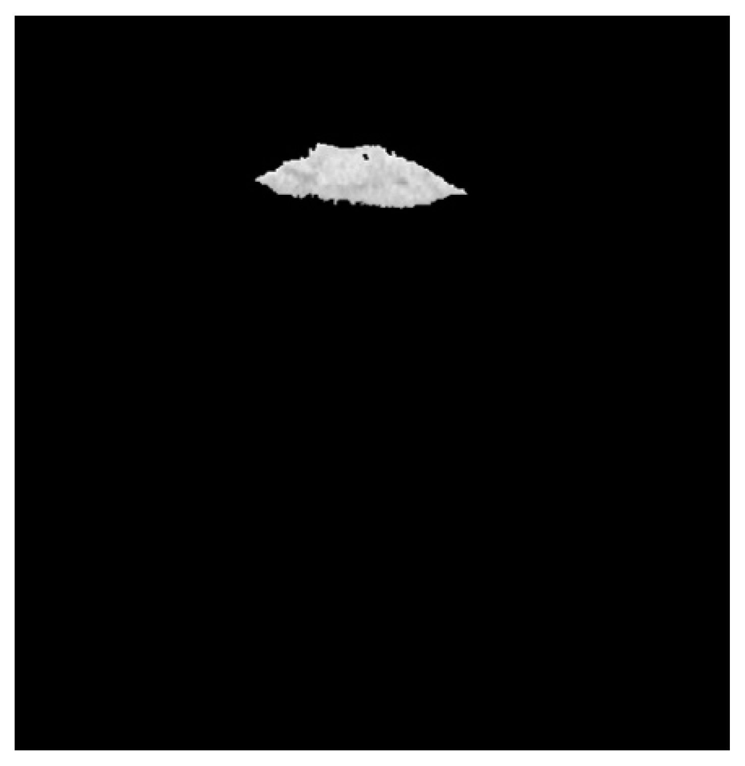
After applying the mathematical morphological operation, there are some pixels, which belong to ROI that are missed accidentally, and those pixels are important to determine the size and the shape of ROI. Thus, using region growing is important to acquire the whole mass. Region growing is a simple region-based image segmentation method. It is also classified as a pixel-based image segmentation method since it involves the selection of initial seed points. The process of region growing begins with a seed region and consequently grows by adding to the seed region those neighboring pixels that have properties similar to the seed region. In our implementation, the seed was chosen by selecting the first pixel in the region that remained after the erosion operation applied in the previous phase. Figure 6 illustrates the result of using the region growing in Figure 5.
Furthermore, it is important to note that the result of applying the above preprocessing and segmentation techniques on normal and abnormal brain images in our dataset resulted in a completely blank image for normal brains, whereas abnormal brain images consisted of some non-black regions. This indicates that we were able to detect brain hemorrhages with 100% accuracy.
2.3. Feature Extraction
Extracting discriminating features from images is one of the most critical steps in building a machine learning-based automated predictor for brain hemorrhage. In our implementation, we applied regionprops function in MATLAB on the ROI obtained after segmentation to compute several useful features. In total, we extracted 17 features from the ROI. These features are briefly described below.
- Area: the actual number of pixels in the ROI. The area of the ROI provides a single scalar feature.
- Bounding Box: the smallest rectangle containing the ROI, which is represented as a 1-by-Q*2 vector, where Q is the number of image dimensions. Suppose that the ROI is represented by the white pixels in Figure 7, then the green box represents the bounding box of the discontinuous ROI. The bounding box of ROI provides four features, which are upper-left corner x-coordinate (ULX), upper-left corner y-coordinate (ULY), width (W), and length (L).
- Centroid: the center of mass of the ROI shown by a red dot in Figure 7. It is represented as a 1-by-Q vector, where Q is the number of image dimensions. The first element of the centroid is the horizontal coordinate or x-coordinate of the center of mass. Likewise, the second element of the centroid is the vertical coordinate or y-coordinate of the center of mass. The centroid of the ROI provides two features (centroid x, centroid y). Figure 7 illustrates the centroid for a discontinuous ROI.
- EquivDiameter: measures the diameter of a circle containing the ROI. The EquivDiameter of ROI provides a single feature and is computed as (11):
- Eccentricity: the eccentricity of an ellipse provides a measure of how nearly circular the ellipse is. It is computed as the ratio of the distance between the foci of the ellipse and its major axis length. In our implementation, eccentricity is used to capture the ROI. It provides a single feature whose value is between 0 and 1. An ellipse whose eccentricity is 0 is actually a circle, while an ellipse whose eccentricity is 1 is a line segment.
- Extent: the ratio of the pixels in the ROI to the pixels in the total bounding box. The extent provides a single feature and is computed as the area divided by the area of the bounding box given, represented as (12):
- Convex Area: the number of pixels in the convex hull of the ROI, where convex hull is the smallest convex polygon that can contain the ROI. The convex area provides a single feature.
- Filled Area: the number of on pixels in the bounding box. The on pixels correspond to the region, with all holes filled in. The filled area provides a single feature.
- Major Axis Length: measures the length (in pixels) of the major axis of the ellipse that includes the ROI. The major axis length provides a single feature.
- Minor Axis Length: measures the length (in pixels) of the minor axis of the ellipse that includes the ROI. The minor axis length provides a single feature.
- Orientation: represents the angle (ranging from −90 to 90 degrees) between the x-axis and the major axis of the ellipse that includes the ROI, as shown in Figure 8. Figure 8 illustrates the axes and orientation of the ellipse. The left side of the figure (Figure 8a) shows an image region and its corresponding ellipse. Likewise, the right side of the figure (Figure 8b) shows the same ellipse with the solid blue lines representing the axes. Furthermore, in Figure 8b, the red dots are the foci, and the orientation is the angle between the horizontal dotted line and the major axis. The orientation also provides a single feature
- Perimeter: represents the distance around the boundary of the ROI. It is computed as the distance between each adjoining pair of pixels around the border of the ROI. The perimeter provides a single feature.
- Solidity: Solidity is given as the proportion of the pixels in the convex hull that is also in the ROI. It is computed as the ratio of area and convex area, represented as (13). The solidity also provides a single feature.
2.4. Feature Selection Using Genetic Algorithm (GA)
The selection of relevant features to train the machine learning-based algorithm is one of the most important steps towards building a robust predictor. In this implementation, we used GA in order to select useful features. GA is a population-based search algorithm that emulates the natural process of evolution. It contains a population of chromosomes. Each chromosome represents a possible solution to the problem under consideration. In GA, first, the population is initialized randomly, then the algorithm progresses by iteratively updating the population through various operators including elitism, crossover, and mutation to discover, prioritize and recombine good building blocks present in parent chromosomes to finally obtain better chromosome [19,20,21].
GA is one of the most advanced methods to select the most useful features from the dataset. There are several advantages of using GA for feature selection, some of which are: (i) it usually performs better than traditional feature selection techniques; (ii) it can manage data sets with a large number of features; (iii) it does not need specific knowledge about the problem under study; (iv) it can be easily parallelized, and (v) it utilizes exploration and exploitation technique which other feature selection methods do not apply.
Configuration of GA requires encoding the solution of the problem under consideration in the form of chromosomes and computing the fitness of the chromosomes. In our configuration of GA, we encode each feature in the feature space by a single bit of 1/0 in a chromosome space where the bit 1/0 represents that the ith feature is either selected or not selected, respectively. The length of the chromosome is set equal to the number of features. Furthermore, we use the 10-fold CV accuracy (ACC) of the SVM classifier with the radial basis function (RBF) kernel as the objective fitness because while testing individual ML methods on our dataset, SVM was found to be the best performing method out of the other individual ML methods. Therefore, objective fitness is defined as:
While computing the fitness, the parameters cost (C), and gamma (γ) of the RBF-kernel SVM were optimized using the grid search technique [22,23]. To compute the fitness of the chromosome, a new data space D is obtained, which only includes the features for which the chromosome bit is 1. The values of the ACC metric of the obj_fit is obtained by performing a 10-fold CV on a new data space D using the RBF-kernel SVM algorithm.
Furthermore, the additional parameters of the GA were configured to a population size of 20, maximum generation to 2000, elite-rate to 5%, crossover-rate to 90%, and mutation-rate to 50%. Primarily, through this GA-based feature selection, only 5 out of 17 features were selected as relevant features. Therefore, it provided us with two-fold benefits: (i) a significant reduction in the number of features; and (ii) selection of relevant features.
2.5. Performance Evaluation Metrics
To evaluate the performance of our predictor, called Accurate Identification of Brain Hemorrhage, abbreviated as AIBH, we use a widely popular 10-fold CV approach [24,25,26]. The process of 10-fold CV involves splitting the dataset into 10 parts, where each of the parts is about the same size. Furthermore, when one fold is kept aside for testing, the remaining 9 folds are used to train the machine learning classifier. The process of training and testing is repeated 10 times, such that each fold is kept aside once for testing. Finally, the test accuracies of each fold are combined to compute the average performance [24]. Table 1 lists the metrics used to evaluate the performance as well as compare our predictor with the existing approaches.
2.6. Prediction Framework
To design an automated predictor for a brain hemorrhage, we adopted the logistics of a stacking-based machine learning approach [27]. In the recent past, a stacking-based technique was successfully applied to solve critical biological problems [28,29,30,31]. Stacking is an ensemble learning approach, which collects information from multiple machine learning methods in different layers and combines them to form a new predictor. The stacking based prediction framework gains improved performance compared to the individual machine learning methods as the information obtained from more than one method minimizes the generalization error. Generally, the stacking framework contains two layers, consisting of the base-layer and the meta-layer. The base-layer contains a set of classifiers C1, C2, …, Cn (also known as base-classifiers), and the meta-layer contains a single classifier. The prediction probabilities from the base-classifiers are combined using a new classifier in the meta-layer to reduce the generalization error. To feed the meta-classifier with useful information on the problem space, the classifiers at the base-level are selected such that their underlying principles of operation are different from one another [28,31].
To choose a set of effective classifiers to use in two different layers of the AIBH stacking framework, we first analyzed the performance of six individual classification algorithms, namely: (i) Support Vector Machines (SVM) [32]; (ii) Random Decision Forest (RDF) [33]; (iii) Extra Tree (ET) [34]; (iv) K-Nearest Neighbor (KNN) [35]; (v) Bagging (BAG), and (vi) Logistic Regression (LogReg). These methods and their configuration details are briefly discussed below.
- SVM: considered as an effective algorithm for the binary prediction that minimizes both the empirical classification error in the training phase and generalized error in the test phase. In this research, we explored an RBF-kernel SVM [32,36] as one of the possible candidates to be used in the stacking framework. SVM performs classification task by maximizing the separating hyperplane between two classes and penalizes the instances on the wrong side of the decision boundary using a cost parameter, C. The RBF kernel parameter, γ and the cost parameter, C were optimized to achieve the best accuracy using a grid search [23] approach. The best values of the parameters found are C = 13.4543 and gamma = 1.6817 and used as representative parameter values for the full dataset.We used a grid search to find the best values for c, gamma. This is a search technique that has been widely used in many machine learning applications when it comes to hyperparameter optimization. There are many reasons which let us use grid search: first, the computational time required to find good parameters by grid search is not much more than that by advanced methods since there are only two parameters. Furthermore, grid search can be easily parallelized because each of (C, γ) is independent. Since doing a complete grid search may still be time-consuming, we used a coarse grid first. After identifying a better region on the grid, a finer grid search on that region was conducted [37].
- RDF: The RDF [33] works by creating a large number of decision trees, each of which is trained on a random sub-samples of the training data. The sub-samples that are used to create a decision tree is designed from a given set of observation of training data by taking ‘x’ observations at random and with replacement (also known as bootstrap sampling). Then, the final prediction results are achieved by aggregating the prediction from the individual decision trees. In our configuration, we used bootstrap samples to construct 1000 trees in the forest, and the rest of the parameters were set as default.
- ET: We explored an extremely randomized tree or extra tree [34] as one of the other possible candidates to be used in the stacking framework. ET works by building randomized decision trees on various sub-samples from the original learning sample and uses averaging to improve the prediction accuracy. We constructed the ET model with 1000 trees, and the quality of a split was measured by the Gini impurity index. The rest of the parameters were set as default.
- KNN: KNN [35] is a non-parametric and lazy learning algorithm. It is called non-parametric as it does not make any assumption for underlying data distribution, rather it creates the model directly from the dataset. Additionally, it is called lazy learning as it does not need any training data points for model generation, rather, it directly uses the training data while testing. KNN works by learning from the k closest training samples in the feature space around a target point. The classification decision is produced based on the majority votes coming from the K nearest neighbors. In this research, the value of k was set to 9, and the rest of the parameters were set as default.
- BAG: BAG [38] is an ensemble method, which operates by forming a class of algorithms that creates several instances of a base classifier on random sub-samples of the training samples and subsequently combines their individual predictions to yield a final prediction. Here, the bagging classifier was fit on multiple subsets of data constructed with repetitions using 1000 decision trees, and the rest of the parameters were set as default.
- LogReg: LogReg [21,35], also referred to as logit or MaxEnt, is a machine learning predictor that measures the relationship between the dependent categorical variable and one or more independent variables by creating an estimation probability using logistic regression. In our implementation, all the parameters of the LogReg predictor were set as default.
To configure the stacking model for the identification of brain hemorrhage types, we evaluated several combinations of the base-classifiers. The choice of base-classifiers is made such that the underlying principle of learning of each of the classifiers is different from one other [28,31,39]. In our application, out of 6 different classifiers, the working principles of BAG, ET, and RDF were the same, i.e., BAG, ET, and RDF are all tree-based methods.
Therefore, we individually added each tree-based method with the methods, KNN, and LogReg to form unique combinations, where no two methods shared the same principle of operations. Furthermore, the classifier that yielded the highest performance among all the other individual classifiers (which is SVM in our implementation) was used in both the base as well as the meta-layer.
For example, in SM2 (see below), BAG was added with KNN, LogReg, and SVM, and all these methods have a unique principle of operation. BAG is a tree-based method, KNN relies on the k-neighbors, LogReg is a regression-based method and SVM works by maximizing the separating hyperplane. Similarly, in SM2, ET was added with KNN, LogReg, and SVM. Likewise, in SM3, RDF was added with KNN, LogReg, and SVM with the same region to select the methods whose underlying principles of operation were different from one another.
Finally, the stacking model that yielded the highest performance was selected as the final predictor of brain hemorrhage types. The set of stacking models evaluated are listed below.
- SM1: KNN, LogReg, BAG in base-layer and SVM in meta-layer,
- SM2: KNN, LogReg, BAG, SVM in base-layer and SVM in meta-layer,
- SM3: KNN, LogReg, ET, SVM in base-layer and SVM in meta-layer and
- SM4: KNN, LogReg, RDF, SVM in base-layer and SVM in meta-layer
In SM1, we used KNN, LogReg, and BAG as the base-classifiers and SVM as the meta-classifier. To test the effect of excluding and including the SVM as the base-classifier, we excluded it from the base-layer of SM1, whereas we included it in the base-layer of SM2, SM3, and SM4. Furthermore, the SVM was used as the meta-layer classifier in all the above configurations because it performed best among all the other individual methods applied in this study. Among the above combinations, in SM2, SM3, and SM4, the tree-based classifiers BAG, ET, and RDF are individually combined with the other three methods, KNN, LogReg, and SVM, to learn different information from the problem space. As mentioned above (see Section 2.4, Feature Selection using GA), only 5 features selected through GA were used to train the base-layer classifiers. Furthermore, before training the meta-layer classifier, the probabilities from each of the base-classifiers were combined with the original 5 features, and once again, the GA feature selection was applied. Then, these selected features were used to train the meta-classifier and obtain the final prediction model for the identification of brain hemorrhage types. While analyzing the 10-fold CVs performance of the above four stacking configurations, we found that all the settings mentioned above resulted in equal performance. Therefore, we arbitrarily selected SM1 as the final AIBH stacking framework, which contains KNN, LogReg, BAG as base-classifiers, and a new SVM as meta-classifier. The classification methods, as well as the stacking framework designed in our work, were constructed and optimized using the python library of Scikit-learn [40].
3. Results
Here, we first present the results of the feature selection. Next, we demonstrate the performance comparison of potential base-classifiers followed by the performance comparison of stacking frameworks. Finally, we report the performance of AIBH on the benchmark dataset.
3.1. Feature Selection
In order to select the relevant features that support the performance of the machine learning method, we adopted a GA-based feature selection approach. Primarily, through this GA based feature selection, only five out of 17 features were selected as relevant features. Therefore, it provided us two-fold benefits: (i) a significant reduction in the number of features; and (ii) selection of relevant features. The selection of relevant features to train the machine learning-based algorithm is one of the most important steps towards building a robust predictor. In this implementation, we used GA in order to select useful features.
Table 2 shows the performance comparison of the individual classifiers before and after feature selection. The results in Table 2 indicate that the performance of ET, RDF, SVM, and KNN methods significantly improved after feature selection. However, the performance of the LogReg method significantly decreased. Furthermore, we observed a similar trend with the BAG method, but the decrease in the performance was less significant.
3.2. Selection of Classifiers for Stacking
To select the classifiers to use in the base and meta-layers of the stacking framework, we analyzed the performance of six different machine learning classifiers: ET, RDF, SVM, LogReg, KNN, and BAG on the CT scan dataset through 10-fold CV approach and only using five features selected through the GA-based feature selection. The performance comparison of the individual classifiers on the CT scan dataset is shown in Table 3.
The performance comparison of the individual classifiers in Table 3 shows that SVM provides the best performance among other classifiers. Specifically, SVM attained ACC, PR, Recall, F1-score and MCC of 98%, 98%, 98%, 0.98 and 0.97, respectively. The significantly high values of PR of 98% and Recall of 98% further support the ACC score of 98% achieved by the SVM. This is not only the case with SVM; the high PR and Recall score of all the other classifiers support the ACC score achieved by the respective classifiers. In addition, since the performance score for each classifier is obtained through 10-fold CV, overfitting is not a concern in our application.
Furthermore, it is evident from Table 3 that SVM obtained 1.03%, 5.38%, 30.67%, 38.03% and 6.52% improvement in accuracy compared to ET, RDF, LogReg, KNN, and BAG classifiers, respectively. Based on the ACC of the classifier, SVM was found to be the highest performing classifier followed by ET, RDF, BAG, LogReg, and KNN. As, in stacking, the prediction probabilities from the base-classifiers are combined using a single new classifier in the meta-layer, we selected SVM as a meta-classifier because it was found to be the highest performing classifier among other classifiers implemented in our work. In addition, the highest performance of SVM further motivated us to use the SVM as one of the base-classifiers. Furthermore, the motivation behind selecting SVM as both a meta-classifier as well as a base-classifier is that it has been successfully applied to solve several other important biological problems [26,41,42,43,44].
Moreover, to select additional classifiers to use at the base-layer, we adopted the guidelines of base-classifier selection in stacking, which indicate that the classifiers should be selected such that their underlying principles of operation are different from one another [28]. Therefore, we used KNN and LogReg as two additional classifiers at the base-layer. Next, we individually added single tree-based ensemble methods, BAG, ET, and RDF as the fourth base-classifier. In one of the stacking models, we did not use SVM as the base-classifier. The reason behind doing so was to assess the impact of using and not using the highest performing method in both the base and the meta-layer. Through this approach, we designed four different combinations of stacking framework, namely, SM1, SM2, SM3, and SM4.
In our implementation, we performed three sets of experiments to identify the best stacking framework for brain hemorrhage type identification. The first set of experiments (Exp1) to evaluate the stacking models was carried out using 17 features originally collected in our study. Next, the second set of experiments (Exp2) was carried out using five features obtained by applying GA-based feature selection on the original 17 features. Consequently, the third set of experiments (Exp3) was carried out by applying an additional GA-based feature selection before the meta-layer classifier was trained. Specifically, in the third set of experiments, instead of directly using the combination of features and probabilities from base-classifiers as inputs to the meta-classifier, as done in Exp1 and Exp2, we apply GA-based feature selection to further select the features and input only the selected features to the meta-classifier. In Table 4, we present the performance comparison of SM1, SM2, SM3, and SM4 stacking models for three different experiments Exp1, Exp2, and Exp3. The performance metrics were computed using the 10-fold CV approach on the CT scan dataset in all the stacking-based experiments.
While comparing the performance of different stacking frameworks from three different experiments, Exp1, Exp2, and Exp3, in Table 4, we found that the performance of stacking frameworks from Exp2 and Exp3 outperform the performance of stacking frameworks from Exp1. This shows that the GA-based feature selection plays an extremely important role in selecting useful features and improving the performance of the predictor.
Furthermore, from Table 4, we found that the performance of models SM2, SM3, and SM4 from Exp2 and Exp3 remains similar. However, the performance of SM1 of Exp3 significantly improves over SM1 of Exp2. Note, in Exp3, feature selection is applied again before the meta-layer classifier is trained, which might have helped the performance of the SM1 of Exp3 to improve.
From Table 4, it is further evident that the SM1 model from Exp3 achieves the highest ACC, PR, Recall, F1-score, and MCC. In particular, SM1 results in ACC, PR, Recall, F1-score, and MCC of 99.5%, 99%, 98.9%, 0.989, and 0.986, respectively. A significantly high and similar value of PR and Recall confirms the reason for the high value of ACC. In addition, since the performance score for each classifier is obtained through 10-fold CV, overfitting is not a concern in our application. In particular, models SM2, SM3, and SM4 from Exp2 and Exp3 attained similar performance. The performance of SM2, SM3, and SM4 models from Exp2 and Exp3 are comparatively higher than that of SM2, SM3, and SM4 models from Exp1. Specifically, ACC, PR, Recall, F1-score, and MCC of SM2, SM3, and SM4 models from Exp2 and Exp3 are 1.0%, 2.1%, 1.9%, 2.06%, and 2.7% higher than of SM2, SM3, and SM4 models from Exp1, respectively.
Moreover, the ACC, PR, Recall, F1-score, and MCC of SM1 model from Exp3 are 2.05%, 4.21%, 4.10%, 4.10%, and 5.68% higher than that of SM1 model from Exp2, respectively. Likewise, the ACC, PR, Recall, F1-score, and MCC of SM1 model from Exp3 are 2.58%, 6.45%, 6.34%, 6.34%, and 8.83% higher than that of SM1 model from Exp1, respectively. As the SM1 stacking model only contains three classifiers in the base layer and its execution time is less compared to the other three stacking models SM2, SM3, and SM4, we select SM1 of Exp3 as our final model for the accurate identification of brain hemorrhage types. The overall design and development of SM1 are summarized in Figure 9. The performance accuracy provided by the SM1 stacking model indicates the robustness of our approach.
We present in Table A3 the performance comparison of SM1, SM2, SM3, and SM4 stacking models for six different experiments Exp3, Exp4, Exp5, Exp6, Exp7, and Exp8. Those experiments have different meta-layers, as shown in that table. Using SVM classifier in the meta-layer attained the highest ACC, PR, Recall, F1-score, and MCC of 0.995, 0.99, 0.989, 0.989, and 0.986, respectively.
3.3. Performance Comparison with Existing Approach
Here we compare the performance of AIBH with an existing best-performing brain hemorrhage type classification method proposed by Al-Ayyoub et al. [5]. In [5], a total of 76 CT images of the human brain were used for the training of brain hemorrhage types using 10-fold CV approach, where 25 images were taken from normal brain, 17 images were taken from epidural hemorrhage, 20 images were taken from subdural hemorrhage, and 14 images were taken from intraparenchymal hemorrhage. Furthermore, in that work, the performance of five different machine learning classifiers, including BayesNet, J48, LogReg, ANN, and SVM, were evaluated. Among the five machine learning classifiers, LogReg was found to attain the highest 10-fold CV performance. In addition, in this proposed work, 100 CT images of the human brain are used for classification of brain hemorrhage types using a 10-fold CV approach where each category (normal brain, epidural hemorrhage, subdural hemorrhage, and intraparenchymal hemorrhage) contains 25 images. Furthermore, only the relevant set of features is selected using GA-based feature selection and used as an input to the stacking-based machine learning framework. The performance comparison of AIBH and Al-Ayyoub et al. is shown in Table 5.
Table 5 shows that the proposed approach: AIBH achieves significantly high ACC, PR, Recall, F1-score, and MCC of 99%, 99%, 98.9%, 0.989, and 0.986, respectively. Additionally, we can see that the AIBH predictor yields a PR of 99%, whereas Al-Ayyoub et al.’s LogReg classifier only attained a PR of 92.5%. Likewise, the AIBH predictor yields a Recall of 98.9%, whereas Al-Ayyoub et al.’s LogReg classifier attained a Recall of 92.2%. Moreover, AIBH results in an F1-score of 0.989 compared to 0.921, given by Al-Ayyoub et al.’s LogReg classifier.
These results indicate that the proposed AIBH predictor can identify the true category of brain hemorrhage type from the image with significantly high accuracy. The higher and closer values of PR, Recall, F1-score, and MCC performance metrics further confirms the robustness and effectiveness of the proposed AIBH predictor. Further, from Table 5, it is also evident that AIBH provides an improvement of 7.03%, 7.27%, and 7.38% compared to Al-Ayyoub et al.’s LogReg classifier based on PR, Recall, and F1-score, respectively. These results indicate a significant improvement over the existing approach. Additionally, these outcomes help us summarize that the AIBH can be effectively used for the detection and diagnosis of brain hemorrhage and ultimately will be useful in teaching, research, and medical purposes.
Moreover, the corresponding analysis and comparison demand a separate but challenging publication assuming we need to connect the generalized complexity of machine learning with the relevant statistical analysis. This is challenging because the separating line between statistical inference and machine learning is subject to debate [45,46].
4. Conclusions
In this work, we have developed a stacking-based machine learning predictor, called AIBH, for the prediction of four different types of brain hemorrhage that includes epidural hemorrhage, subdural hemorrhage, intraparenchymal hemorrhage, and normal brains. We collected a benchmark dataset that contains a total of 100 CT scan images, with 25 images in each category, to train and validate the proposed AIBH method. Our approach succeeded in removing all undesired regions and retrieving the region of interest (brain hemorrhage region).
To summarize, first, we converted the images from the RGB scale to grayscale and then removed the white pixels (skull region). Second, we segmented the image into three regions using Otsu’s method. Thus, we could determine the ROI and remove undesired regions. Third, we extracted 17 features for the ROI, such as the size of the ROI, centroid of the ROI, perimeter of the ROI, and more. Finally, we utilized the GA based feature selection, and an advanced machine learning technique called stacking to ensure highly accurate brain hemorrhage type identification. The nobility of our approach is demonstrated by AIBH attaining an ACC of 99.5%, PR of 99%, Recall of 98.9%, F1-score of 0.989, and MCC of 0.986, respectively.
Author Contributions
Data collection and processing D.M.A. Conceived and designed the experiments: D.M.A., A.M., and M.T.H. Performed the experiments: D.M.A. and A.M. Analyzed the data: D.M.A., A.M. and M.T.H. Contributed reagents/materials/analysis tools: M.T.H. Wrote the paper: D.M.A., A.M., and M.T.H. All authors have read and agreed the publication of the final version of the manuscript.
Funding
The authors gratefully acknowledge the Louisiana Board of Regents through the Board of Regents Support Fund LEQSF (2016-19)-RD-B-07.
Conflicts of Interest
The authors declare no conflicts of interest.
Appendix A

Table A1.
Class-wise and average values of performance metrics of individual machine learning methods on CT scan dataset before and after feature selection.
Table A1.
Class-wise and average values of performance metrics of individual machine learning methods on CT scan dataset before and after feature selection.
| Before Feature Selection | ||||||
| Evaluation Metrics | ||||||
| Classifier | Hemorrhage Type | ACC | PR | Recall | F1-Score | MCC |
| ET | Epidural | 0.88 | 0.88 | 0.88 | 0.88 | 0.84 |
| Subdural | 0.96 | 0.92 | 0.96 | 0.94 | 0.92 | |
| Intraparenchymal | 0.92 | 0.96 | 0.92 | 0.94 | 0.92 | |
| Normal | 1 | 1 | 1 | 1 | 1 | |
| Average | 0.94 | 0.94 | 0.94 | 0.94 | 0.92 | |
| RDF | Epidural | 0.8 | 0.87 | 0.80 | 0.83 | 0.78 |
| Subdural | 0.96 | 0.92 | 0.96 | 0.94 | 0.92 | |
| Intraparenchymal | 0.92 | 0.88 | 0.92 | 0.90 | 0.87 | |
| Normal | 1 | 1 | 1 | 1 | 1 | |
| Average | 0.92 | 0.92 | 0.92 | 0.92 | 0.89 | |
| SVM | Epidural | 0.92 | 0.88 | 0.92 | 0.90 | 0.87 |
| Subdural | 0.96 | 0.96 | 0.96 | 0.96 | 0.95 | |
| Intraparenchymal | 0.92 | 0.96 | 0.92 | 0.94 | 0.92 | |
| Normal | 1 | 1 | 1 | 1 | 1 | |
| Average | 0.95 | 0.95 | 0.95 | 0.95 | 0.93 | |
| LogReg | Epidural | 0.76 | 0.76 | 0.76 | 0.76 | 0.68 |
| Subdural | 0.96 | 0.83 | 0.96 | 0.89 | 0.85 | |
| Intraparenchymal | 0.72 | 0.86 | 0.72 | 0.78 | 0.72 | |
| Normal | 1 | 1 | 1 | 1 | 1 | |
| Average | 0.86 | 0.86 | 0.86 | 0.86 | 0.82 | |
| KNN | Epidural | 0.56 | 0.50 | 0.56 | 0.53 | 0.36 |
| Subdural | 0.88 | 0.79 | 0.88 | 0.83 | 0.77 | |
| Intraparenchymal | 0.32 | 0.44 | 0.32 | 0.37 | 0.21 | |
| Normal | 1 | 0.96 | 1 | 0.98 | 0.97 | |
| Average | 0.69 | 0.67 | 0.69 | 0.68 | 0.59 | |
| BAG | Epidural | 0.8 | 0.91 | 0.80 | 0.85 | 0.81 |
| Subdural | 0.96 | 0.92 | 0.96 | 0.94 | 0.92 | |
| Intraparenchymal | 0.96 | 0.89 | 0.96 | 0.92 | 0.90 | |
| Normal | 1 | 1 | 1 | 1 | 1 | |
| Average | 0.93 | 0.93 | 0.93 | 0.93 | 0.91 | |
| After Feature Selection | ||||||
| ET | Epidural | 0.88 | 1 | 0.88 | 0.94 | 0.92 |
| Subdural | 1 | 0.96 | 1 | 0.98 | 0.97 | |
| Intraparenchymal | 1 | 0.93 | 1 | 0.96 | 0.95 | |
| Normal | 1 | 1 | 1 | 1 | 1 | |
| Average | 0.97 | 0.97 | 0.97 | 0.97 | 0.96 | |
| RDF | Epidural | 0.8 | 0.91 | 0.80 | 0.85 | 0.81 |
| Subdural | 0.96 | 0.92 | 0.96 | 0.94 | 0.92 | |
| Intraparenchymal | 0.96 | 0.89 | 0.96 | 0.92 | 0.90 | |
| Normal | 1 | 1 | 1 | 1 | 1 | |
| Average | 0.93 | 0.93 | 0.93 | 0.93 | 0.91 | |
| SVM | Epidural | 0.92 | 1 | 0.92 | 0.96 | 0.95 |
| Subdural | 1 | 0.93 | 1 | 0.96 | 0.95 | |
| Intraparenchymal | 1 | 1 | 1 | 1 | 1 | |
| Normal | 1 | 1 | 1 | 1 | 1 | |
| Average | 0.98 | 0.98 | 0.98 | 0.98 | 0.97 | |
| LogReg | Epidural | 0.48 | 0.52 | 0.48 | 0.50 | 0.34 |
| Subdural | 1 | 0.76 | 1 | 0.86 | 0.82 | |
| Intraparenchymal | 0.52 | 0.68 | 0.52 | 0.59 | 0.49 | |
| Normal | 1 | 1 | 1 | 1 | 1 | |
| Average | 0.75 | 0.74 | 0.75 | 0.74 | 0.67 | |
| KNN | Epidural | 0.4 | 0.45 | 0.40 | 0.43 | 0.25 |
| Subdural | 0.88 | 0.81 | 0.88 | 0.85 | 0.79 | |
| Intraparenchymal | 0.56 | 0.54 | 0.56 | 0.55 | 0.39 | |
| Normal | 1 | 1 | 1 | 1 | 1 | |
| Average | 0.71 | 0.70 | 0.71 | 0.71 | 0.61 | |
| BAG | Epidural | 0.76 | 0.90 | 0.76 | 0.83 | 0.78 |
| Subdural | 0.96 | 0.89 | 0.96 | 0.92 | 0.90 | |
| Intraparenchymal | 0.96 | 0.89 | 0.96 | 0.92 | 0.90 | |
| Normal | 1 | 1 | 1 | 1 | 1 | |
| Average | 0.92 | 0.92 | 0.92 | 0.92 | 0.89 | |
Table A2.
Class-wise and average values of performance metrics of stacking models on CT scan dataset for three different experiments, Exp1, Exp2 and Exp3.
Table A2.
Class-wise and average values of performance metrics of stacking models on CT scan dataset for three different experiments, Exp1, Exp2 and Exp3.
| Exp1 | ||||||
| Evaluation Metrics | ||||||
| Stacking Models | Hemorrhage Type | ACC | PR | Recall | F1-Score | MCC |
| SM1 | Epidural | 0.930 | 0.846 | 0.880 | 0.851 | 0.863 |
| Subdural | 0.980 | 0.960 | 0.960 | 0.941 | 0.960 | |
| Intraparenchymal | 0.950 | 0.916 | 0.880 | 0.923 | 0.897 | |
| Normal | 1.00 | 1.00 | 1.00 | 1.00 | 1.00 | |
| Average | 0.965 | 0.930 | 0.930 | 0.928 | 0.930 | |
| SM2 | Epidural | 0.970 | 0.958 | 0.92 | 0.938 | 0.919 |
| Subdural | 0.980 | 0.960 | 0.96 | 0.96 | 0.946 | |
| Intraparenchymal | 0.990 | 0.961 | 1.00 | 0.980 | 0.974 | |
| Normal | 1.00 | 1.00 | 1.00 | 1.00 | 1.00 | |
| Average | 0.985 | 0.969 | 0.970 | 0.969 | 0.959 | |
| SM3 | Epidural | 0.970 | 0.958 | 0.92 | 0.938 | 0.919 |
| Subdural | 0.980 | 0.960 | 0.96 | 0.960 | 0.946 | |
| Intraparenchymal | 0.990 | 0.961 | 1.00 | 0.980 | 0.974 | |
| Normal | 1.00 | 1.00 | 1.00 | 1.00 | 1.00 | |
| Average | 0.985 | 0.969 | 0.970 | 0.969 | 0.959 | |
| SM4 | Epidural | 0.970 | 0.958 | 0.92 | 0.938 | 0.919 |
| Subdural | 0.980 | 0.960 | 0.96 | 0.960 | 0.946 | |
| Intraparenchymal | 0.990 | 0.961 | 1.00 | 0.980 | 0.974 | |
| Normal | 1.00 | 1.00 | 1.00 | 1.00 | 1.00 | |
| Average | 0.985 | 0.969 | 0.970 | 0.969 | 0.959 | |
| Exp2 | ||||||
| SM1 | Epidural | 0.950 | 0.884 | 0.920 | 0.901 | 0.868 |
| Subdural | 0.980 | 0.960 | 0.960 | 0.960 | 0.946 | |
| Intraparenchymal | 0.970 | 0.958 | 0.920 | 0.938 | 0.919 | |
| Normal | 1.00 | 1.00 | 1.00 | 1.00 | 1.00 | |
| Average | 0.975 | 0.950 | 0.950 | 0.950 | 0.933 | |
| SM2 | Epidural | 0.990 | 1.00 | 0.960 | 0.979 | 0.973 |
| Subdural | 0.990 | 0.961 | 1.00 | 0.980 | 0.974 | |
| Intraparenchymal | 1.00 | 1.00 | 1.00 | 1.00 | 1.00 | |
| Normal | 1.00 | 1.00 | 1.00 | 1.00 | 1.00 | |
| Average | 0.995 | 0.990 | 0.99 | 0.989 | 0.986 | |
| SM3 | Epidural | 0.990 | 1.00 | 0.960 | 0.979 | 0.973 |
| Subdural | 0.990 | 0.961 | 1.00 | 0.980 | 0.974 | |
| Intraparenchymal | 1.00 | 1.00 | 1.00 | 1.00 | 1.00 | |
| Normal | 1.00 | 1.00 | 1.00 | 1.00 | 1.00 | |
| Average | 0.995 | 0.990 | 0.99 | 0.989 | 0.986 | |
| SM4 | Epidural | 0.990 | 1.00 | 0.960 | 0.979 | 0.973 |
| Subdural | 0.990 | 0.961 | 1.00 | 0.980 | 0.974 | |
| Intraparenchymal | 1.00 | 1.00 | 1.00 | 1.00 | 1.00 | |
| Normal | 1.00 | 1.00 | 1.00 | 1.00 | 1.00 | |
| Average | 0.995 | 0.990 | 0.99 | 0.989 | 0.986 | |
| Exp3 | ||||||
| SM1 | Epidural | 0.989 | 1.00 | 0.958 | 0.978 | 0.972 |
| Subdural | 0.989 | 0.961 | 1.00 | 0.980 | 0.974 | |
| Intraparenchymal | 1.00 | 1.00 | 1.00 | 1.00 | 1.00 | |
| Normal | 1.00 | 1.00 | 1.00 | 1.00 | 1.00 | |
| Average | 0.995 | 0.990 | 0.989 | 0.989 | 0.986 | |
| SM2 | Epidural | 0.989 | 1.00 | 0.958 | 0.978 | 0.972 |
| Subdural | 0.989 | 0.961 | 1.00 | 0.980 | 0.974 | |
| Intraparenchymal | 1.00 | 1.00 | 1.00 | 1.00 | 1.00 | |
| Normal | 1.00 | 1.00 | 1.00 | 1.00 | 1.00 | |
| Average | 0.995 | 0.990 | 0.989 | 0.989 | 0.986 | |
| SM3 | Epidural | 0.989 | 1.00 | 0.958 | 0.978 | 0.972 |
| Subdural | 0.989 | 0.961 | 1.00 | 0.980 | 0.974 | |
| Intraparenchymal | 1.00 | 1.00 | 1.00 | 1.00 | 1.00 | |
| Normal | 1.00 | 1.00 | 1.00 | 1.00 | 1.00 | |
| Average | 0.995 | 0.990 | 0.989 | 0.989 | 0.986 | |
| SM4 | Epidural | 0.989 | 1.00 | 0.958 | 0.978 | 0.972 |
| Subdural | 0.989 | 0.961 | 1.00 | 0.980 | 0.974 | |
| Intraparenchymal | 1.00 | 1.00 | 1.00 | 1.00 | 1.00 | |
| Normal | 1.00 | 1.00 | 1.00 | 1.00 | 1.00 | |
| Average | 0.995 | 0.990 | 0.989 | 0.989 | 0.986 | |
Table A3.
Class-wise and average values of performance metrics of stacking models on CT scan dataset for different experiments, Exp1, Exp4, Exp5, Exp6, Exp7, and Exp8, with different classifiers in meta-layer.
Table A3.
Class-wise and average values of performance metrics of stacking models on CT scan dataset for different experiments, Exp1, Exp4, Exp5, Exp6, Exp7, and Exp8, with different classifiers in meta-layer.
| Stacking Models | Meta Layer | Num. of Features in Base-Layer | Num. of Features in Meta-Layer | Evaluation Metrics | |||||
|---|---|---|---|---|---|---|---|---|---|
| ACC | PR | Recall | F1-Score | MCC | |||||
| Exp1 | SM1 | SVM | 17 | 29 | 0.995 | 0.990 | 0.989 | 0.989 | 0.986 |
| SM2 | SVM | 17 | 33 | 0.995 | 0.990 | 0.989 | 0.989 | 0.986 | |
| SM3 | SVM | 17 | 33 | 0.995 | 0.990 | 0.989 | 0.989 | 0.986 | |
| SM4 | SVM | 17 | 33 | 0.995 | 0.990 | 0.989 | 0.989 | 0.986 | |
| Exp4 | SM1 | ET | 17 | 29 | 0.991 | 0.990 | 0.990 | 0.939 | 0.986 |
| SM2 | ET | 17 | 33 | 0.991 | 0.990 | 0.990 | 0.939 | 0.986 | |
| SM3 | ET | 17 | 33 | 0.962 | 0.960 | 0.960 | 0.960 | 0.946 | |
| SM4 | ET | 17 | 33 | 0.991 | 0.990 | 0.990 | 0.939 | 0.986 | |
| Exp5 | SM1 | BAGGING | 17 | 29 | 0.941 | 0.940 | 0.940 | 0.9465 | 0.939 |
| SM2 | BAGGING | 17 | 33 | 0.941 | 0.940 | 0.940 | 0.9465 | 0.939 | |
| SM3 | BAGGING | 17 | 33 | 0.962 | 0.960 | 0.960 | 0.960 | 0.946 | |
| SM4 | BAGGING | 17 | 33 | 0.941 | 0.940 | 0.940 | 0.9465 | 0.939 | |
| Exp6 | SM1 | KNN | 17 | 29 | 0.790 | 0.790 | 0.780 | 0.780 | 0.722 |
| SM2 | KNN | 17 | 33 | 0.790 | 0.790 | 0.780 | 0.780 | 0.722 | |
| SM3 | KNN | 17 | 33 | 0.739 | 0.720 | 0.730 | 0.730 | 0.727 | |
| SM4 | KNN | 17 | 33 | 0.706 | 0.680 | 0.690 | 0.690 | 0.601 | |
| Exp7 | SM1 | LOG | 17 | 29 | 0.840 | 0.840 | 0.840 | 0.843 | 0.788 |
| SM2 | LOG | 17 | 33 | 0.840 | 0.840 | 0.840 | 0.843 | 0.788 | |
| SM3 | LOG | 17 | 33 | 0.945 | 0940 | 0940 | 0940 | 0.919 | |
| SM4 | LOG | 17 | 33 | 0.810 | 0.800 | 0.810 | 0.80 | 0.749 | |
| Exp8 | SM1 | RAND | 17 | 29 | 0.941 | 0.940 | 0.940 | 0.940 | 0.920 |
| SM2 | RAND | 17 | 33 | 0.941 | 0.940 | 0.940 | 0.940 | 0.920 | |
| SM3 | RAND | 17 | 33 | 0.962 | 0.960 | 0.960 | 0.960 | 0.946 | |
| SM4 | RAND | 17 | 33 | 0.941 | 0.940 | 0.940 | 0.940 | 0.920 | |
Table A4.
Class-wise and average values of performance metrics of stacking models on CT scan dataset for two different experiments, Exp2 and Exp 9.
Table A4.
Class-wise and average values of performance metrics of stacking models on CT scan dataset for two different experiments, Exp2 and Exp 9.
| Evaluation Metrics | |||||||
|---|---|---|---|---|---|---|---|
| Stacking Models | Hemorrhage Type | ACC | Stacking Models | Hemorrhage Type | ACC | ||
| Exp2 | SM2 | Epidural | 0.990 | 1.00 | 0.960 | 0.979 | 0.973 |
| Subdural | 0.990 | 0.961 | 1.00 | 0.980 | 0.974 | ||
| Intraparenchymal | 1.00 | 1.00 | 1.00 | 1.00 | 1.00 | ||
| Normal | 1.00 | 1.00 | 1.00 | 1.00 | 1.00 | ||
| Average | 0.995 | 0.990 | 0.99 | 0.989 | 0.986 | ||
| Exp 9 | SM2 | Epidural | 0.990 | 1.00 | 0.960 | 0.979 | 0.99 |
| Subdural | 0.990 | 0.961 | 1.00 | 0.980 | 0.99 | ||
| Intraparenchymal | 1.00 | 1.00 | 1.00 | 1.00 | 1.00 | ||
| Normal | 1.00 | 1.00 | 1.00 | 1.00 | 1.00 | ||
| Average | 0.995 | 0.990 | 0.99 | 0.989 | 0.995 | ||
References
- Ali Khairat, M.W. Epidural Hematoma. In StatPearls; StatPearls Publishing: Treasure Island, FL, USA, 2019. [Google Scholar]
- CASP12. Available online: http://predictioncenter.org/casp12/index.cgi (accessed on 20 January 2019).
- Gong, T.; Liu, R.; Tan, C.L.; Farzad, N.; Lee, C.K.; Pang, B.C.; Tian, Q.; Tang, S.; Zhang, Z. Classification of CT Brain Images of Head Trauma. In Proceedings of the 2nd IAPR International Conference on Pattern Recognition in Bioinformatics, Singapore, 1–2 October 2007; pp. 401–408. [Google Scholar]
- Sapra, P.; Singh, R.; Khurana, S. Brain tumor detection using Neural Network. Int. J. Sci. Mod. Eng. 2013, 1, 83–88. [Google Scholar]
- Al-Ayyoub, M.; Alawad, D.; Al-Darabsah, K.; Aljarrah, I. Automatic detection and classification of brain hemorrhages. WSEAS Trans. Comput. 2013, 12, 395–405. [Google Scholar]
- Phong, T.D.; Duong, H.N.; Nguyen, H.T.; Trong, N.T.; Nguyen, V.H.; Hoa, T.V.; Snasel, V. Brain Hemorrhage Diagnosis by Using Deep Learning. In Proceedings of the 2017 International Conference on Machine Learning and Soft Computing, Ho Chi Minh City, Vietnam, 13–16 January 2017. [Google Scholar]
- Sharma, B.; Venugopalan, K. Classification of Hematomas in Brain CT Images Using Neural Network. In Proceedings of the 2014 International Conference on Issues and Challenges in Intelligent Computing Techniques (ICICT), Ghaziabad, India, 7–8 February 2014. [Google Scholar]
- Filho, P.P.R.; Sarmento, R.M.; Holanda, G.B.; de Alencar Lima, D. New approach to detect and classify stroke in skull CT images via analysis of brain tissue densities. Comput. Methods Programs Biomed. 2017, 148, 27–43. [Google Scholar] [CrossRef] [PubMed]
- Roy, S.; Saha, A.; Bandyopadhyay, S.K. Brain tumor segmentation and quantification from MRI of brain. J. Glob. Res. Comput. Sci. 2011, 2, 155–160. [Google Scholar]
- Mahajan, R.; Mahajan, P.M. Survey On Diagnosis Of Brain Hemorrhage By Using Artificial Neural Network. Int. J. Sci. Res. Eng. Technol. 2016, 5, 378–381. [Google Scholar]
- Shahangian, B.; Pourghassem, H. Automatic Brain Hemorrhage Segmentation and Classification in CTscan Images. In Proceedings of the 2013 8th Iranian Conference on Machine Vision and Image Processing, Zanjan, Iran, 10–12 September 2013. [Google Scholar]
- Garg, H. A hybrid GSA-GA algorithm for constrained optimization problems. Inf. Sci. 2019, 478, 499–523. [Google Scholar] [CrossRef]
- Shelke, V.R.; Rajwade, R.A.; Kulkarni, M. Intelligent Acute Brain Hemorrhage Diagnosis System. In Proceedings of the International Conference on Advances in Computer Science, AETACS, NCR, India, 13–14 December 2013. [Google Scholar]
- Garg, H.; Kaur, G. Quantifying gesture information in brain hemorrhage patients using probabilistic dual hesitant fuzzy sets with unknown probability information. Comput. Ind. Eng. 2020, 140, 106211. [Google Scholar] [CrossRef]
- Kerekes, Z.; Tóth, Z.; Szénási, S.; Tóth, Z.; Sergyán, S. Colon Cancer Diagnosis on Digital Tissue Images. In Proceedings of the 2013 IEEE 9th International Conference on Computational Cybernetics (ICCC), Tihany, Hungary, 8–10 July 2013. [Google Scholar]
- Al-Darabsah, K.; Al-Ayyoub, M. Breast Cancer Diagnosis Using Machine Learning Based on Statistical and Texture Features Extraction. In Proceedings of the 4th International Conference on Information and Communication Systems (ICICS 2013), Irbid, Jordan, 23–25 April 2013. [Google Scholar]
- Otsu, N. A threshold selection method from gray-level histograms. IEEE Trans. Syst. Man Cybern. 1979, 9, 62–66. [Google Scholar] [CrossRef] [Green Version]
- Srisha, R.; Khan, A. Morphological Operations for Image Processing: Understanding and Its Applications. In Proceedings of the National Conference on VLSI, Signal processing & Communications, Vignans University, Guntur, India, 11–12 December 2013. [Google Scholar]
- Hoque, M.T.; Iqbal, S. Genetic algorithm-based improved sampling for protein structure prediction. Int. J. Bio-Inspired Comput. 2017, 9, 129–141. [Google Scholar] [CrossRef]
- Hoque, M.T.; Chetty, M.; Sattar, A. Protein Folding Prediction in 3D FCC HP Lattice Model Using Genetic Algorithm. In Proceedings of the IEEE Congress on Evolutionary Computation (CEC), Singapore, 25–28 September 2007; pp. 4138–4145. [Google Scholar]
- Hoque, M.T.; Chetty, M.; Lewis, A.; Sattar, A.; Avery, V.M. DFS Generated Pathways in GA Crossover for Protein Structure Prediction. Neurocomputing 2010, 73, 2308–2316. [Google Scholar] [CrossRef] [Green Version]
- Frey, D.J.; Mishra, A.; Hoque, M.T.; Abdelguerfi, M.; Soniat, T. A machine learning approach to determine oyster vessel behavior. Mach. Learn. Knowl. Extr. 2018, 1, 4. [Google Scholar] [CrossRef] [Green Version]
- Bergstra, J.; Bengio, Y. Random search for hyper-parameter optimization. J. Mach. Learn. Res. 2012, 13, 281–305. [Google Scholar]
- Hastie, T.; Tibshirani, R.; Friedman, J. The Elements of Statistical Learning, 2nd ed.; Springer: New York, NY, USA, 2009. [Google Scholar]
- Bishop, C. Pattern Recognition and Machine Learning; Springer: New York, NY, USA, 2009. [Google Scholar]
- Iqbal, S.; Mishra, A.; Hoque, T. Improved Prediction of Accessible Surface Area Results in Efficient Energy Function Application. J. Theor. Biol. 2015, 380, 380–391. [Google Scholar] [CrossRef]
- Wolpert, D.H. Stacked generalization. Neural Netw. 1992, 5, 241–259. [Google Scholar] [CrossRef]
- Mishra, A.; Pokhrel, P.; Hoque, M.T. StackDPPred: A stacking based prediction of DNA-binding protein from sequence. Bioinformatics 2019, 35, 433–441. [Google Scholar] [CrossRef] [PubMed]
- Iqbal, S.; Hoque, M.T. PBRpredict-Suite: A suite of models to predict peptide-recognition domain residues from protein sequence. Bioinformatics 2018, 34, 3289–3299. [Google Scholar] [CrossRef] [PubMed] [Green Version]
- Nagi, S.; Bhattacharyya, D.K. Classification of microarray cancer data using ensemble approach. Netw. Model. Anal. Health Inform. Bioinform. 2013, 2, 159–173. [Google Scholar] [CrossRef] [Green Version]
- Gattani, S.; Mishra, A.; Hoque, M.T. StackCBPred: A stacking based prediction of protein-carbohydrate binding sites from sequence. Carbohydr. Res. 2019, 486, 107857. [Google Scholar] [CrossRef]
- Cortes, C.; Vapnik, V. Support-vector networks. Mach. Learn. 1995, 20, 273–297. [Google Scholar] [CrossRef]
- Ho, T.K. Random Decision Forests. In Proceedings of the Third International Conference on Document Analysis and Recognition, Montreal, QC, Canada, 14–16 August 1995; pp. 278–282. [Google Scholar]
- Geurts, P.; Ernst, D.; Wehenkel, L. Extremely randomized trees. Mach. Learn. 2006, 63, 3–42. [Google Scholar] [CrossRef] [Green Version]
- Altman, N.S. An Introduction to Kernel and Nearest-Neighbor Nonparametric Regression. Am. Stat. 1992, 46, 175–185. [Google Scholar]
- Vapnik, V.N. An overview of statistical learning theory. IEEE Trans. Neural Netw. 1999, 10, 988–999. [Google Scholar] [CrossRef] [PubMed] [Green Version]
- Hsu, C.W.; Chang, C.C.; Lin, C.-J. A Practical Guide to Support Vector Classication; Department of Computer Science, National Taiwan University: Taipei, Taiwan, 2010; pp. 1–12. [Google Scholar]
- Breiman, L. Bagging predictors. Mach. Learn. 1996, 24, 123–140. [Google Scholar] [CrossRef] [Green Version]
- Ma, Z.; Wang, P.; Gao, Z.; Wang, R.; Khalighi, K. Ensemble of machine learning algorithms using the stacked generalization approach to estimate the warfarin dose. PLoS ONE 2018, 13, e0205872. [Google Scholar] [CrossRef] [Green Version]
- Pedregosa, F.; Varoquaux, G.; Gramfort, A.; Michel, V.; Thirion, B.; Grisel, O.; Blondel, M.; Prettenhofer, P.; Weiss, R.; Dubourg, V.; et al. Scikit-learn: Machine Learning in Python. J. Mach. Learn. Res. 2011, 12, 2825–2830. [Google Scholar]
- Xu, R.; Zhou, J.; Wang, H.; He, Y.; Wang, X.; Liu, B. Identifying DNA-binding proteins by combining support vector machine and PSSM distance transformation. BMC Syst. Biol. 2015, 9, S10. [Google Scholar] [CrossRef] [Green Version]
- Taherzadeh, G.; Yang, Y.; Zhang, T.; Liew, A.W.C.; Zhou, Y. Sequence-based prediction of protein–peptide binding sites using support vector machine. J. Comput. Chem. 2016, 37, 1223–1229. [Google Scholar] [CrossRef] [Green Version]
- Liua, H.-L.; Chen, S.-C. Prediction of disulfide connectivity in proteins with support vector machine. J. Chin. Inst. Chem. Eng. 2007, 38, 63–70. [Google Scholar] [CrossRef]
- Kumar, R.; Srivastava, A.; Kumari, B.; Kumar, M. Prediction of β-lactamase and its class by Chou’s pseudo-amino acid composition and support vector machine. J. Theor. Biol. 2015, 365, 96–103. [Google Scholar] [CrossRef]
- Bzdok, D. Classical Statistics and Statistical Learning in Imaging Neuroscience. Front. Neurosci. 2017, 11, 543. [Google Scholar] [CrossRef] [PubMed]
- Bzdok, D.; Altman, N.; Krzywinski, M. Points of significance: Statistics versus machine learning. Nat. Methods 2018, 15, 233–234. [Google Scholar] [CrossRef] [PubMed]
Figure 1.
(a) Normal brain image is compared with the three types of hemorrhage: (b) epidural hemorrhage, (c) intraparenchymal hemorrhage, and (d) subdural hemorrhage.
Figure 1.
(a) Normal brain image is compared with the three types of hemorrhage: (b) epidural hemorrhage, (c) intraparenchymal hemorrhage, and (d) subdural hemorrhage.
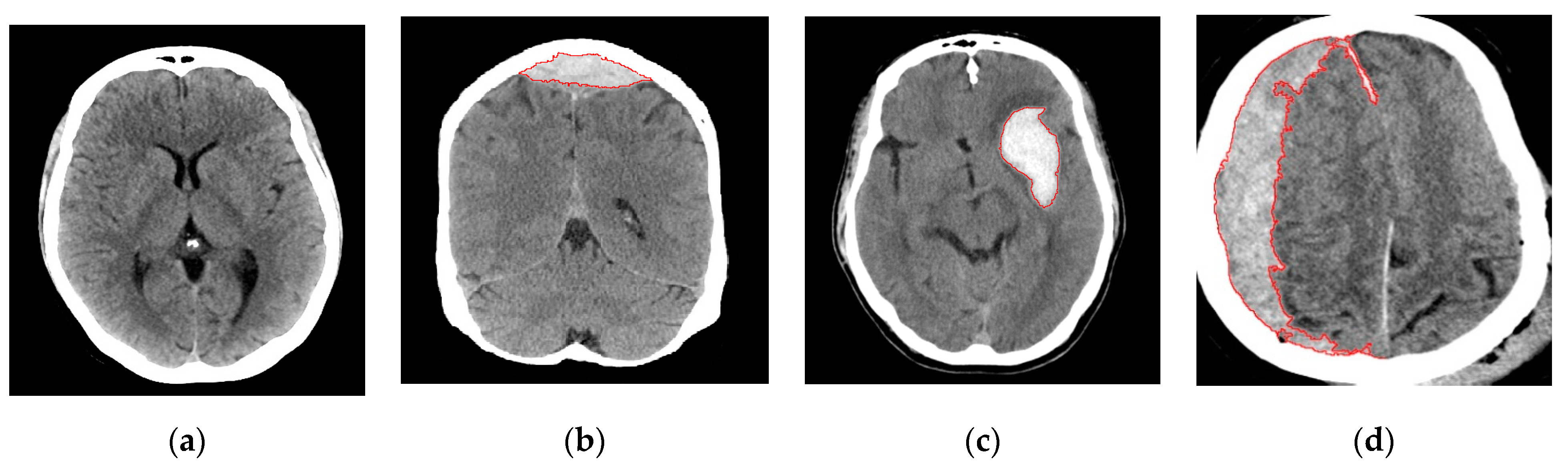
Figure 2.
Illustration of computed tomography (CT) images (a) before and (b) after removing the skull.
Figure 2.
Illustration of computed tomography (CT) images (a) before and (b) after removing the skull.

Figure 3.
Illustration of images obtained (a) before and (b) after applying Otsu’s segmentation method.
Figure 3.
Illustration of images obtained (a) before and (b) after applying Otsu’s segmentation method.
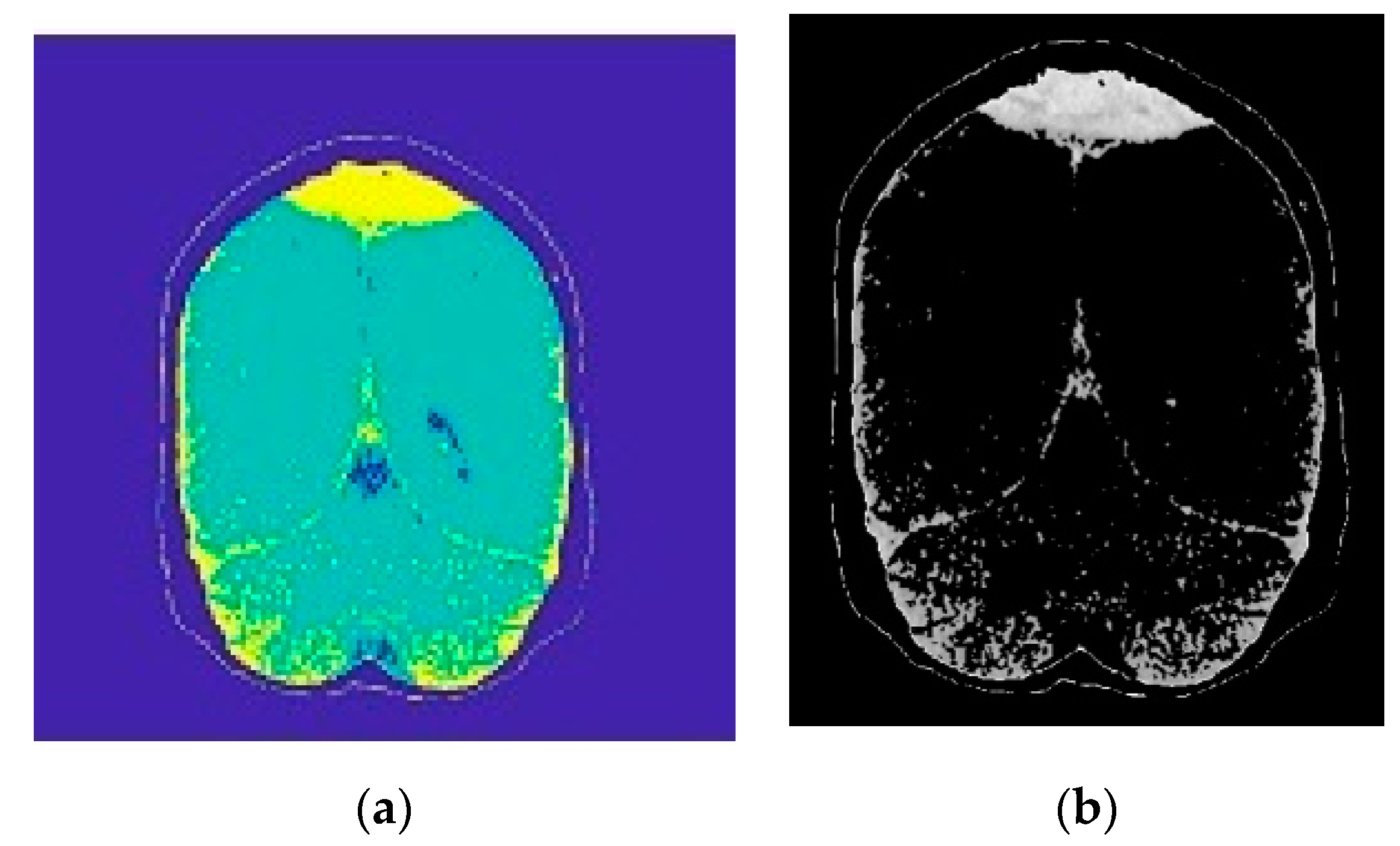
Figure 4.
The flat disk-shaped structuring element used in this work.
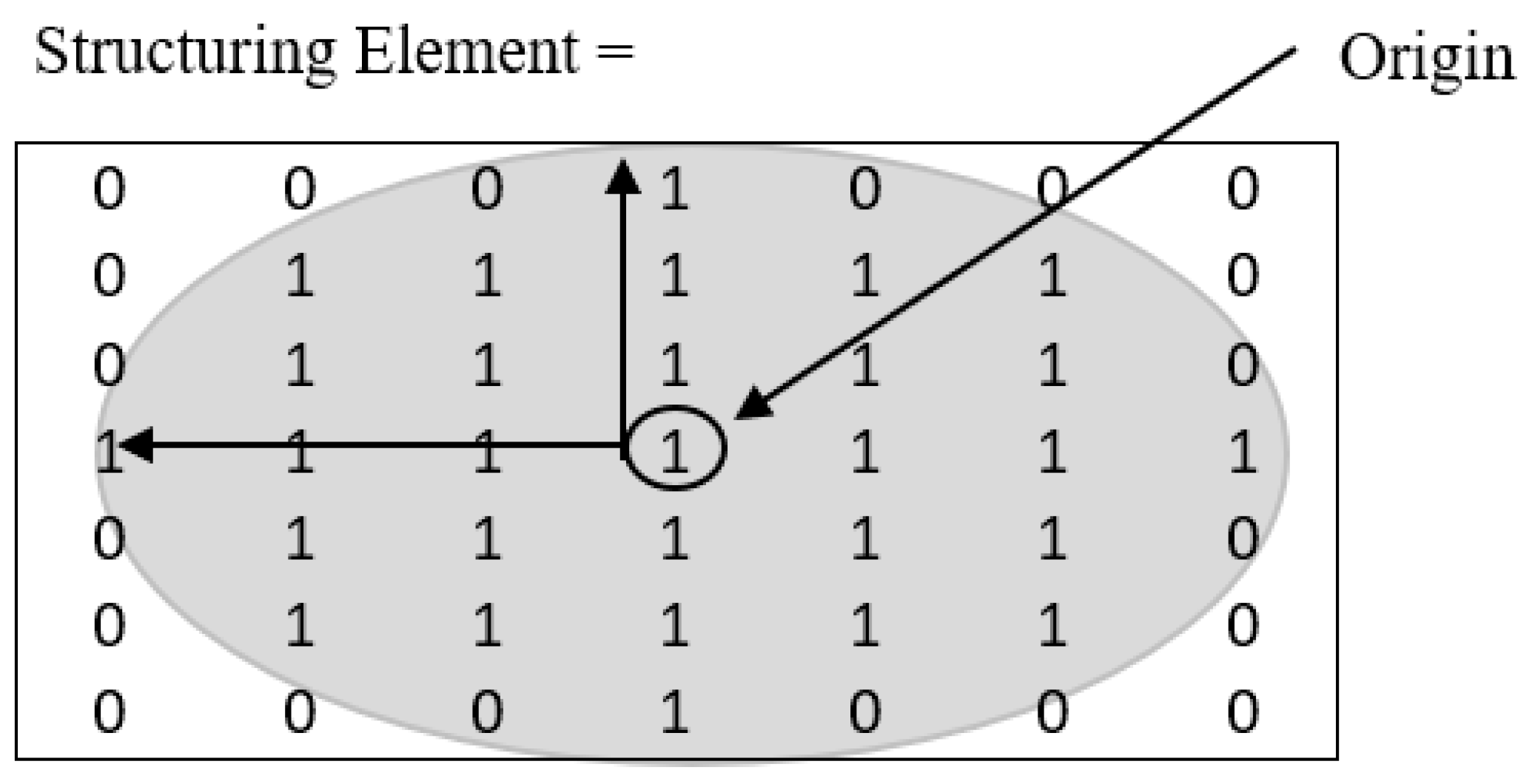
Figure 5.
The result after applying erosion operation.
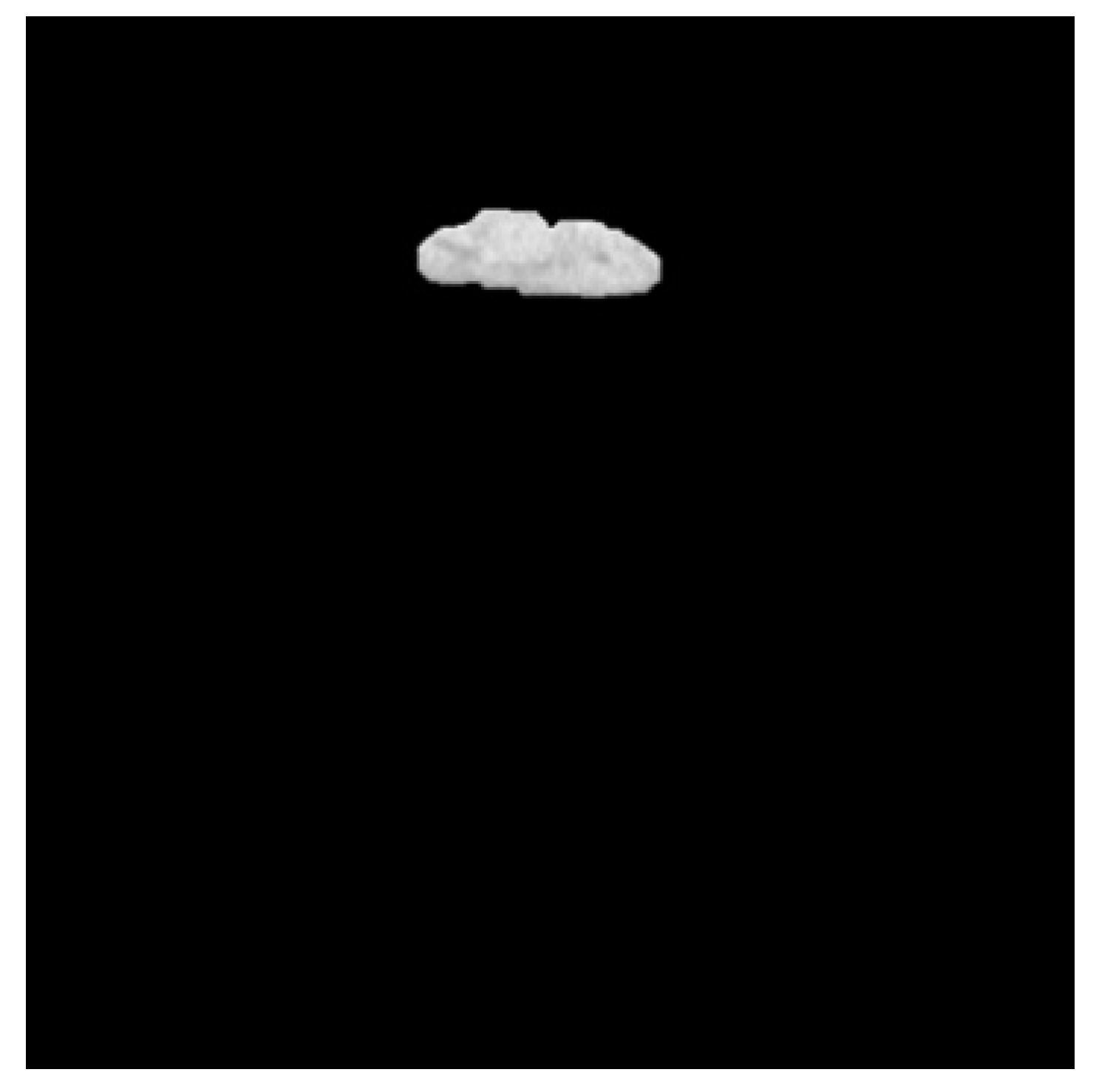
Figure 6.
The result, after applying the region growing in Figure 5.
Figure 6.
The result, after applying the region growing in Figure 5.

Figure 7.
The centroid (red dot) and the bounding box (green box) of the discontinuous region of interest (ROI).
Figure 7.
The centroid (red dot) and the bounding box (green box) of the discontinuous region of interest (ROI).
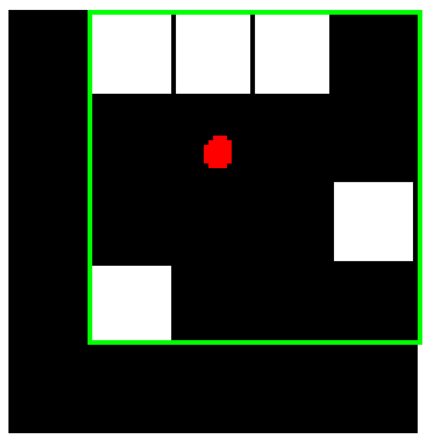
Figure 8.
(a) Ellipse fitting the pixels, (b) the angle between the x-axis and major axis of the fitted ellipse forms the orientation feature.
Figure 8.
(a) Ellipse fitting the pixels, (b) the angle between the x-axis and major axis of the fitted ellipse forms the orientation feature.
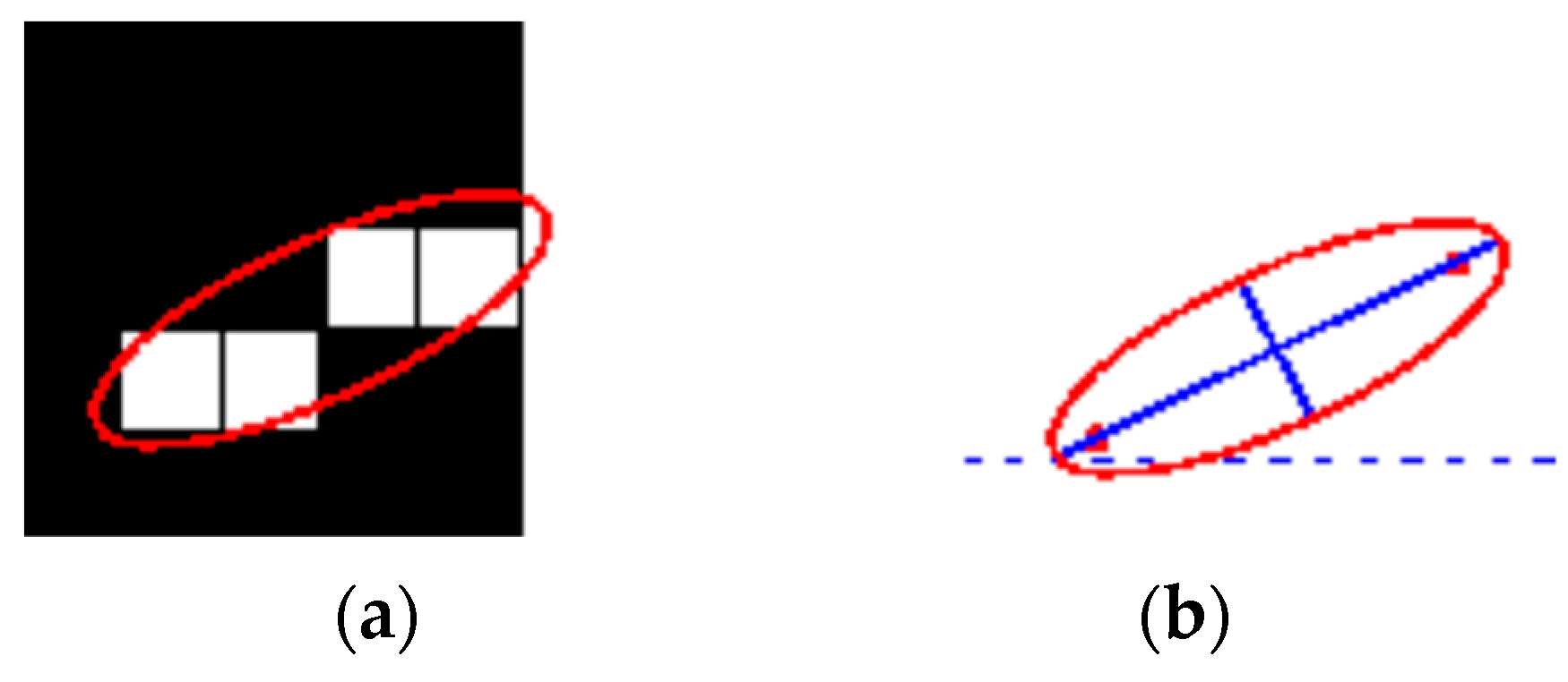
Figure 9.
The overall design and development of the final model, SM1, which is a four-class classification framework. The input of the model is a brain image, and outputs are the probabilities of the four classes: epidural hemorrhage, subdural hemorrhage, intraparenchymal hemorrhage, and normal or healthy brain.
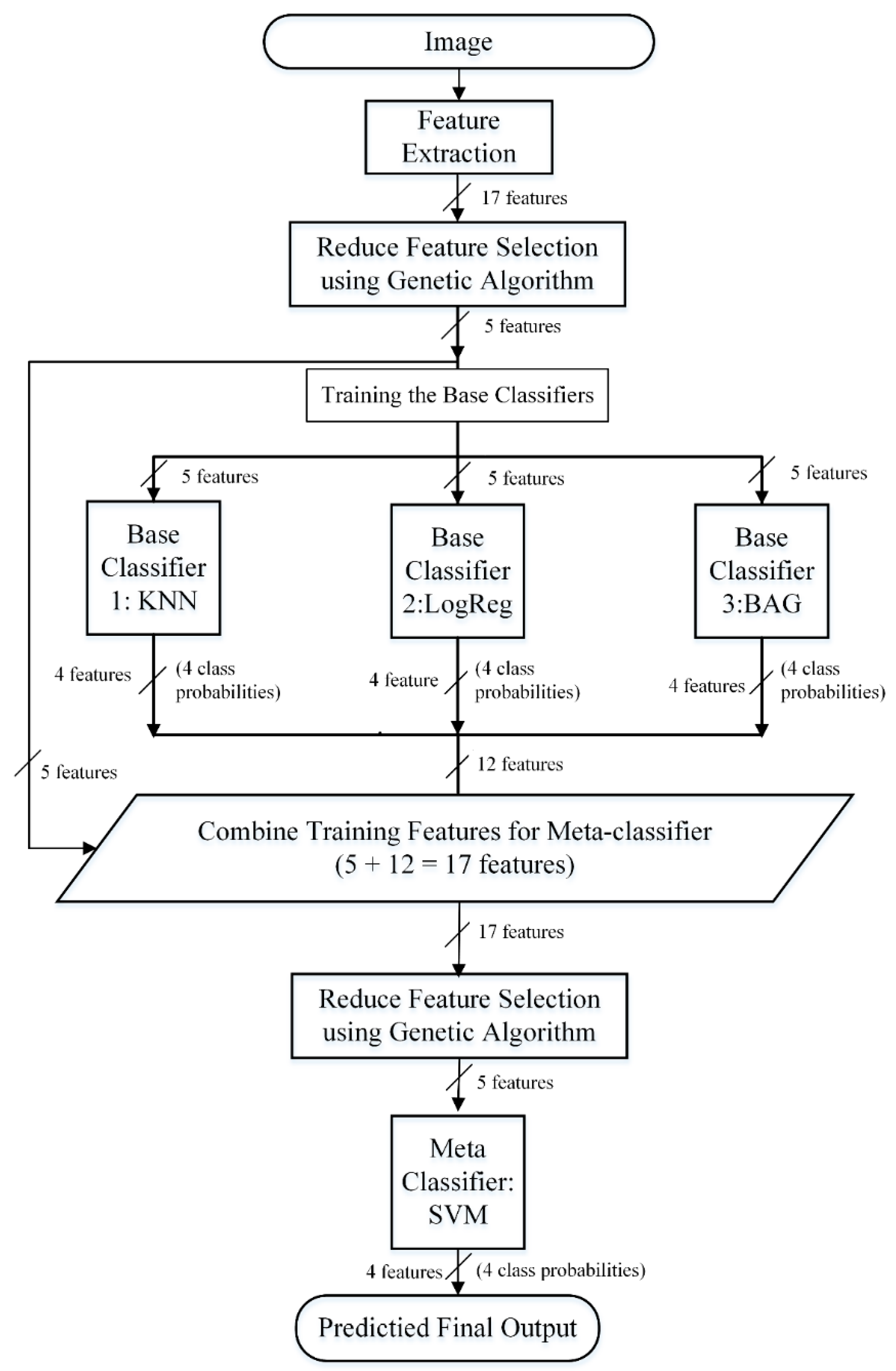
Table 1.
Name and definition of the performance evaluation metrics.
| Name of Metric | Definition |
|---|---|
| True positive (TP) | Correctly predicted type of Brain hemorrhage |
| True negative (TN) | Correctly predicted other type of Brain hemorrhage |
| False positive (FP) | Incorrectly predicted Brain hemorrhage type |
| False negative (FN) | Incorrectly predicted other type of Brain hemorrhage |
| Recall/Sensitivity/True Positive Rate (TPR) | |
| Accuracy (ACC) | |
| Precision | |
| F1 score (Harmonic mean of precision and recall) | |
| Mathews Correlation Coefficient (MCC) |
Table 2.
Comparison of prediction results of individual machine learning methods on CT scan dataset before and after feature selection (see Appendix A, Table A1 for further details).
Table 2.
Comparison of prediction results of individual machine learning methods on CT scan dataset before and after feature selection (see Appendix A, Table A1 for further details).
| Algorithm | Num. of Features | Evaluation Metrics | |||||
|---|---|---|---|---|---|---|---|
| ACC | PR | Recall | F1-Score | MCC | |||
| Before Feature Selection | ET | 17 | 0.94 | 0.94 | 0.94 | 0.94 | 0.92 |
| RDF | 17 | 0.92 | 0.92 | 0.92 | 0.92 | 0.89 | |
| SVM | 17 | 0.95 | 0.95 | 0.95 | 0.95 | 0.93 | |
| LogReg | 17 | 0.86 | 0.86 | 0.86 | 0.86 | 0.82 | |
| KNN | 17 | 0.69 | 0.67 | 0.69 | 0.68 | 0.59 | |
| BAG | 17 | 0.93 | 0.93 | 0.93 | 0.93 | 0.91 | |
| After GA-based Feature Selection | ET | 5 | 0.97 | 0.97 | 0.97 | 0.97 | 0.96 |
| RDF | 5 | 0.93 | 0.93 | 0.93 | 0.93 | 0.91 | |
| SVM | 5 | 0.98 | 0.98 | 0.98 | 0.98 | 0.97 | |
| LogReg | 5 | 0.75 | 0.74 | 0.75 | 0.74 | 0.67 | |
| KNN | 5 | 0.71 | 0.70 | 0.71 | 0.71 | 0.61 | |
| BAG | 5 | 0.92 | 0.92 | 0.92 | 0.92 | 0.89 | |
Note: The comparison is performed between individual methods before and after feature selection, and the best scores are boldfaced.
Table 3.
Comparison of various machine learning algorithms on the CT scan dataset through the 10-fold cross-validation (CV).
Table 3.
Comparison of various machine learning algorithms on the CT scan dataset through the 10-fold cross-validation (CV).
| Metric/Methods | ET | RDF | SVM | LogReg | KNN | BAG |
|---|---|---|---|---|---|---|
| ACC | 0.97 | 0.93 | 0.98 | 0.75 | 0.71 | 0.92 |
| PR | 0.97 | 0.93 | 0.98 | 0.74 | 0.70 | 0.92 |
| Recall | 0.97 | 0.93 | 0.98 | 0.75 | 0.71 | 0.92 |
| F1-score | 0.97 | 0.93 | 0.98 | 0.74 | 0.71 | 0.92 |
| MCC | 0.96 | 0.91 | 0.97 | 0.67 | 0.61 | 0.89 |
Note: Best score values are boldfaced.
Table 4.
Comparison of different stacking models on the CT scan dataset through the 10-fold CV (see Appendix A, Table A2 for further details).
Table 4.
Comparison of different stacking models on the CT scan dataset through the 10-fold CV (see Appendix A, Table A2 for further details).
| Stacking Models | Num. of Features in Base-Layer | Num. of Features in Meta-Layer | Evaluation Metrics | |||||
|---|---|---|---|---|---|---|---|---|
| ACC | PR | Recall | F1-Score | MCC | ||||
| Exp1 | SM1 | 17 | 29 | 0.965 | 0.930 | 0.930 | 0.928 | 0.930 |
| SM2 | 17 | 33 | 0.985 | 0.969 | 0.970 | 0.969 | 0.959 | |
| SM3 | 17 | 33 | 0.985 | 0.969 | 0.970 | 0.969 | 0.959 | |
| SM4 | 17 | 33 | 0.985 | 0.969 | 0.970 | 0.969 | 0.959 | |
| Exp2 | SM1 | 5 | 17 | 0.975 | 0.950 | 0.950 | 0.950 | 0.933 |
| SM2 | 5 | 21 | 0.995 | 0.990 | 0.990 | 0.989 | 0.986 | |
| SM3 | 5 | 21 | 0.995 | 0.990 | 0.990 | 0.989 | 0.986 | |
| SM4 | 5 | 21 | 0.995 | 0.990 | 0.990 | 0.989 | 0.986 | |
| Exp3 | SM1 | 5 | 5 | 0.995 | 0.990 | 0.989 | 0.989 | 0.986 |
| SM2 | 5 | 6 | 0.995 | 0.990 | 0.989 | 0.989 | 0.986 | |
| SM3 | 5 | 8 | 0.995 | 0.990 | 0.989 | 0.989 | 0.986 | |
| SM4 | 5 | 7 | 0.995 | 0.990 | 0.989 | 0.989 | 0.986 | |
The comparison is performed between the stacking models of three different experiments, and the best scores are boldfaced.
Table 5.
Comparison of AIBH with existing Al-Ayyoub et al. method.
| Metric/Methods | Al-Ayyoub et al. | AIBH (% imp.) |
|---|---|---|
| ACC | - | 0.995 (-) |
| PR | 0.925 | 0.990 (7.03%) |
| Recall | 0.922 | 0.989 (7.27%) |
| F1-score | 0.921 | 0.989 (7.38%) |
| MCC | - | 0.986 (-) |
Note: Best score values are boldfaced. The “-” indicates a missing value.
© 2020 by the authors. Licensee MDPI, Basel, Switzerland. This article is an open access article distributed under the terms and conditions of the Creative Commons Attribution (CC BY) license (http://creativecommons.org/licenses/by/4.0/).
Share and Cite
MDPI and ACS Style
Alawad, D.M.; Mishra, A.; Hoque, M.T. AIBH: Accurate Identification of Brain Hemorrhage Using Genetic Algorithm Based Feature Selection and Stacking. Mach. Learn. Knowl. Extr. 2020, 2, 56-77. https://doi.org/10.3390/make2020005
AMA Style
Alawad DM, Mishra A, Hoque MT. AIBH: Accurate Identification of Brain Hemorrhage Using Genetic Algorithm Based Feature Selection and Stacking. Machine Learning and Knowledge Extraction. 2020; 2(2):56-77. https://doi.org/10.3390/make2020005
Chicago/Turabian StyleAlawad, Duaa Mohammad, Avdesh Mishra, and Md Tamjidul Hoque. 2020. "AIBH: Accurate Identification of Brain Hemorrhage Using Genetic Algorithm Based Feature Selection and Stacking" Machine Learning and Knowledge Extraction 2, no. 2: 56-77. https://doi.org/10.3390/make2020005