1. Introduction
High-dimensional models with correlated predictors are commonly seen in practice. Most statistical models work well either in low-dimensional correlated case, or in high-dimensional independent case. There are few methods that deal with high-dimensional correlated predictors, which usually have limited theoretical and practical capacity. Neural networks have been applied in practice for years, which have a good performance under correlated predictors. The reason is that the non-linearity and interactions are brought in by the activation functions and nodes in the hidden layers. A universal approximation theorem guarantees that a single-layer artificial neural network is able to approximate any continuous function with an arbitrarily small approximation error, provided that there is a large enough number of hidden nodes in the architecture. Thus, the artificial neural network (ANN) handles the correlation and interactions automatically and implicitly. A popular machine learning application that deals with this type of dependency is the spatio-temporal data, where the traditional statistical methods model the spatial covariance matrix of the predictors. However, by artificial neural networks, working with this big covariance matrix can be avoided. Moreover, artificial neural networks also have good performance in computer vision tasks in practice.
A main drawback of neural networks is that it requires a huge number of training sample due to large number of inherent parameters. In some application fields, such as clinical trials, brain imaging data analysis and some computer vision applications, it is usually hard to obtain such a large number of observations in the training sample. Thus, there is a need for developing high-dimensional neural networks with regularization or dimension reduction techniques. It is known that
norm regularization [
26] shrinks insignificant parameters to zero. Commonly used regularization includes
norm regularization, for example, see the keras package [
6].
norm regularization with
controls the model sensitivity [
15]. On the other hand
norm regularization with
, where people usually take
for computation efficiency, does not encourage group information. The group lasso regularization [
27] yields group-wise sparseness while keeping parameters dense within the groups. A common regularization used in high-dimensional artificial neural network is the sparse group lasso by [
21], see for example [
11], which is a weighted combination of the lasso regularization and the group lasso regularization. The group lasso regularization part penalizes the input features’ weights group-wisely: A feature is either selected or dropped, and it is connected to all nodes in the hidden layer if selected. The lasso part further shrinks some weights of the selected inputs features to zero: A feature does not need to be connected to all nodes in the hidden layer when selected. This penalization encourages as many zero weights as possible. Another common way to overcome the high-dimensionality is to add dropout layers [
23]. Randomly setting parameters in the later layers to zero keeps less non-zero estimations and reduces the variance. Dropout layer is proved to work well in practice, but no theoretical guarantee is available. [
17] considers a deep network with the combination of regularization in the first layer and dropout in other layers. With a deep representation, neural networks have more approximation power which works well in practice. They propose a fast and stable algorithm to train the deep network. However, no theoretical guarantee is given for the proposed method other than practical examples.
On the other hand, though widely used, high-dimensional artificial neural networks still do not have a solid theoretical foundation for statistical validation, especially in the case of classification. Typical theory for low-dimensional ANNs traces back to the 1990s, including [
1,
2,
8,
25]. The existing results include the universal approximation capabilities of single layer neural networks, the estimation and classification consistency under the Gaussian assumption and 0-1 loss in the low dimensional case. These theory assumes the 0-1 loss which is not used nowadays and are not sufficient for high-dimensional case as considered here. Current works focus more on developing new computing algorithms rather building theoretical foundations or only have limited theoretical foundations. [
11] derived a convergence rate of the log-likelihood function in the neural network model, but this does not guarantee the universal classification consistency or the convergence of the classification risk. The convergence of the log-likelihood function is necessary but not sufficient for the classification risk to converge. In this paper, we obtained consistency results of classification risk for high-dimensional artificial neural networks. We derived the convergence rate for the prediction error, and proved that under mild conditions, the classification risk of a high-dimensional artificial neural network classifier actually tends to the optimal Bayes classifier’s risk. This type of property has been established on other classifiers such as KNN [
7], which derived the result that the classification risk of KNN tends to the Bayes risk, LDA [
28], which derives the classification error rate under Gaussian assumptions, etc. Popular tasks, like analyzing MRI data and computer vision models, were also included in these research papers, and we applied the high-dimensional neural network to these demanding tasks as well.
In
Section 2, we will formulate the problem and the high-dimensional neural network formally. In
Section 3, we state the assumptions and the main consistency result. In
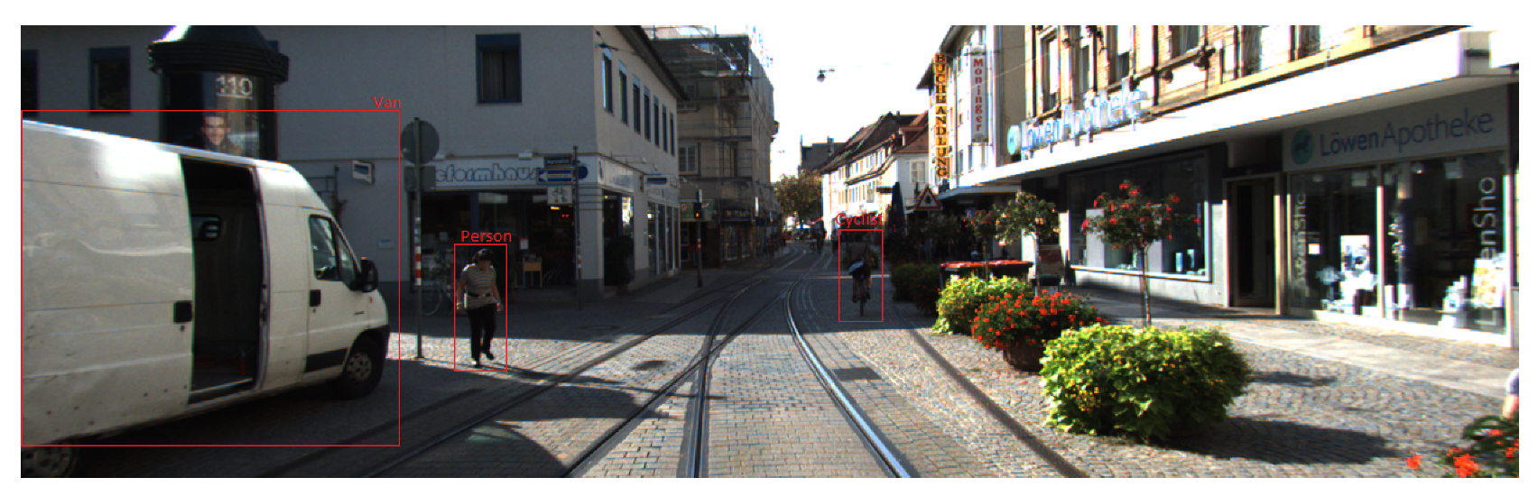
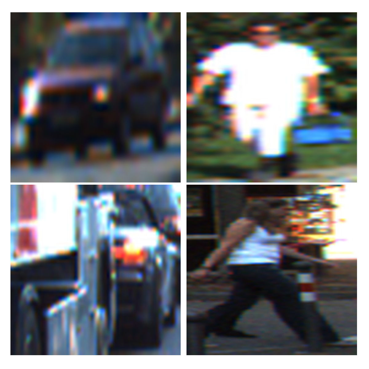
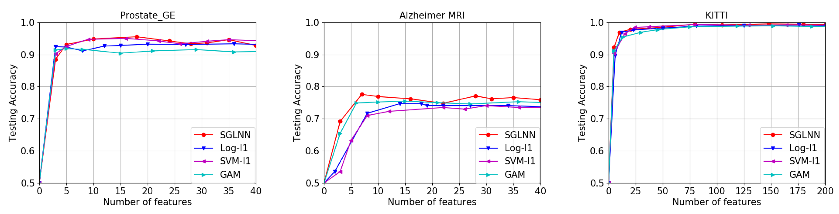
Section 5, we apply the high-dimensional neural network in three different aspects of examples: the gene data, the MRI data and the computer vision data. In
Section 6, further ideas are discussed.
2. The Binary Classification Problem
Consider the binary classification problem
where
is the feature vector drawn from the feature space according to some distribution
, and
is some continuous function. Note here that, in the function
, there can be any interactions among the predictors in
, which ensures the possibility to handle correlated predictors. Let
be the joint distribution on
, where
and
. Here
p could be large, and may be even larger than the training sample size
n. To study the theory, we assume
p has some relationship with
n, for example,
. Therefore,
p should be written as
, which indicates the dependency. However, for simplicity, we suppress the notation
and denote it with
p.
For a new observation
, the Bayes classifier, denoted
, predicts 1 if
and 0 otherwise, where
is a probability threshold, which is usually chosen as
in practice. The Bayes classifier is proved to minimize the risk
However, the Bayes classifier is not useful in practice, since is unknown. Thus a classifier is to be found based on the observations , which are drawn from . A good classifier based on the sample should have its risk tend to the Bayes risk as the number of observations tends to infinity, without any requirement for its probability distribution. This is the so-called universal consistency.
Multiple methods have been adopted to estimate
, including the logistic regression (a linear approximation), generalized additive models (GAM, a non-parametric nonlinear approximation which does not take interactions into account), neural networks (a complicated structure which is dense in continuous functions space), etc. The first two methods usually work in practice with a good theoretical foundation, however, they sometimes fail to catch the complicated dependency among the feature vector
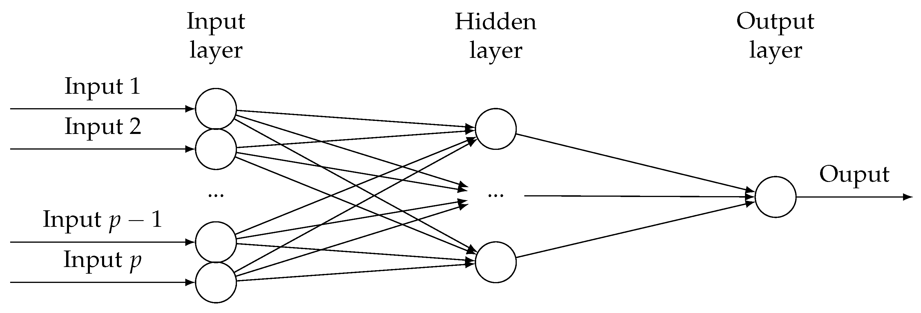
in a wide range of applications (brain images, computer visions and spatial data analysis). The neural network structure is proved to be able to capture this dependency implicitly without explicitly specifying the dependency hyper-parameters. Consider a single layer neural network model with
p predictor variables. The hidden layer has
nodes, where
may be a diverging sequence depending on
n. Similar to
, we suppress
as
m. A diagram is shown in
Figure 1.
For an input vector
, its weight matrix
and its hidden layer intercept vector
, let the vector
be the corresponding values in the hidden nodes, which is defined as
Let
be an activation function, then the output for a given set of weight
is calculated by
where the function
is the function
being applied element-wisely. We have a wide range of choices for the activation function. [
16] proved that as long as the activation is not algebraic polynomials, the single layer neural network is dense in the continuous function space, and can thus be used to approximate any continuous function. This structure can be considered as a model which, for a given activation function
, maps a
input vector to an real-valued output
where
is the output of the single hidden layer neural network with parameter
. Applying the logistic function
,
as an approximation of
with parameters
where
. According to the universal approximation theorem, see [
8], with a big enough
m, the single layer neural network is able to approximate any continuous function with a quite small approximation error.
By [
2], assuming that there is a Fourier representation of
of the form
, let
for some bounded subset of
containing zero and for some constant
. Then for all functions
, there exists a single layer neural network output
such that
on
B. Later [
20] generalizes the result by relaxing the assumptions on the activation function and improved the rate of approximation by a logarithmic factor. They showed that on a bounded domain
with Lipschitz boundary, assuming
satisfies
for some extension
with
, if the activation function
is non-zero and satisfies the polynomial decay condition
for some
and some
, we have
where the norm is in Sobolev space of order
r, and
is a function of
s,
r,
and
only. Both results ensure the good approximation property of single layer neural network, and the convergence rate is independent of the dimension of
,
p, as long as
f has a Fourier transform which decays sufficiently fast.
Towards building the high-dimensional ANN, we start by formalizing the model. Let
be a
design or input matrix,
let
be a
response or outcome vector,
let
be a
parameter or input weight matrix,
let
be a
parameter vector,
let
be a
parameter vector representing node weights,
and let
b be a scalar parameter.
When one tries to bring neural network into the high-dimension set up, or equivalently, the small sample size scenario, it usually does not work well. The estimability issue [
14] arise from the fact that even a single layer neural network may have too many parameters. This issue might already exist in the low dimensional case (
), let alone the high dimension case. A single layer neural network usually includes
parameters, which is possible to be much more than the training sample size
n. In practice, a neural network may work well with one of the local optimal solutions although this is not guaranteed by theory. Regularization methods can be applied to help obtain a sparse solution. On one hand, proper choice of regularization shrinks partial parameters to zero, which addresses the statistical estimability issue. On the other hand, regularization makes the model more robust.
Assuming sparsity is usually the most efficient way of dealing with the high dimensionality. A lasso type regularization on the parameters has been shown numerically to have poor performance on neural network models. On one hand, lasso does not drop a feature entirely but only disconnect it with some hidden nodes. On the other hand, lasso does not select dependent predictor variables in a good manner [
9]. Consider the sparse group lasso proposed by [
21], which penalizes the predictors group-wise and individually simultaneously. It is a combination of the group lasso and the lasso, see for example [
11]. The group lasso regularization part penalizes the input features’ weights group-wisely: a feature is either selected or dropped, and it is connected to all nodes in the hidden layer if selected. The lasso part further shrinks some weights of the selected inputs features to zero: a feature does not need to be connected to all nodes in the hidden layer when selected.
Define the loss function as the log-likelihood function
Besides the sparse group lasso regularization, we consider a
regularization on other parameters. Then we have
such that
The sparse group lasso penalty [
11,
21] includes a group lasso part and a lasso part, which are balanced using the hyper-parameter
. The group lasso part treats each input as group of
m variables, including the weights for the
m hidden nodes connected to each input. This regularization will be able to include or drop an input variable’s
m hidden nodes group-wisely [
27]. The lasso regularization is used to further make the weights sparse within each group, i.e., each input selected by the group lasso regularization does not have to connect to all hidden nodes. This combination of the two regularizations makes the estimation even easier for small sample problems. The
norm regularization on the other parameters is more about practical concerns, since it further reduces the risk of overfitting.
Though with slight difference on the regularization, [
11] proposed a fast coordinate gradient descent algorithm for the estimation, which cycles the gradient descent for the differentiable part of the loss function, the threshold function for the group lasso part and the threshold function for the lasso part. Three tuning parameters,
,
and
K can be selected with cross-validations on a grid search.
3. The Consistency of Neural Network Classification Risk
In this section, we conduct the theoretical investigation of classification accuracy of the neural network model. Before stating the theorems, we need a few assumptions. The independence property of neural networks, see [
1,
25] and [
11], states that the first-layer weights in
satisfy
and
the set of dilated and translated functions
is linearly independent.
The independence property means that different nodes depend on the input predictor variables through different linear combinations and none of the hidden nodes is a linear combination of the other nodes, which is crucial in the universal approximation capability of neural networks. [
20] proved that the above set is linearly independent if
are pairwise linearly independent, as long as the non-polynomial activation function is an integrable function which satisfies a polynomial growth condition.
According to [
11], if the parameters
satisfy the independence property, the following equivalence class of parameters
contains only parameterizations that are sign-flips or rotations and has cardinality exactly
.
Let
be the distribution of
Y for fixed
and
be the empirical measure. The best approximation in the neural network space is the equivalence class of parameters by minimizing the population loss
where
is the loss function with parameters
. Let
Q be the number of equivalent classes in
. The Excess loss is defined as
where
is a set of parameters in
. Moreover, when we refer to a set of parameters in
for some parameter
, we mean that
has the minimum distance to
. [
11] has shown that this excess loss plus the estimation of the irrelevant weights is bounded from above and may tend to zero with proper choices of
n,
p and the tuning parameters.
Another concern is the estimability of the parameters. A common remedy is to assume sparsity of the predictors. Thus we make the following assumption.
Assumption 1. (Sparsity) Only s of the predictors are relevant in predicting y (without loss of generality, we assume the first s predictors, denoted S are relevant, and the rest, denoted, are irrelevant), all weights in θ associated with, denoted, are zero in the optimal neural network.
The next assumption is a standard assumption in generalized models, which controls the variance of the response from below and above. Consider a general exponential family distribution on y with canonical function , common assumptions is to bound and from above and below. However, in binary classification problems, these functions are automatically bounded from above by 1, thus we only need to assume the boundedness from below. Some literature assume constant bounds on these quantities, however, we do allow the bounds to change with n and the bounds may tend to zero as n goes to infinity.
Assumption 2. (Boundedness of variance) The true conditional probability of y for a givenis bounded away from 0 and 1 by a quantity, which might tend to zero.
The following two assumptions are inherited from [
11]. The next assumption is a relatively weak assumption on the local convexity of the parameters.
Assumption 3. (Local convexity) There is a constantthat may depend on m, s, f and the distribution, but does not depend on p such that for all, we havewheremeans thatis a positive semi-definite matrix. The next assumption is made to bound the excess loss from below for the parameters outside , i.e., the true model is identifiable. Let be the minimum distance from an element in to , then we assume
Assumption 4. (Identifiability) For all, there is anthat may depend on m, s, f and the distribution, but does not depend on p such that Assumption 3 states that though neural network is a non-convex optimization problem globally, the parameters of the best neural network approximation of the true function has a locally convex neighborhood. The assumption can be assured in this way. By the continuity of the representation of the neural network and the loss function, the integration in Assumption 3 is infinitely continuously differentiable with respect to the nonzero parameters, therefore the second derivative is a continuous function of the nonzero parameters. By the definition of the parameters of the best neural network approximation, minimizes the integration in Assumption 3. If there is not a positive that satisfies assumption, it either contradicts with the fact that the second derivative is continuous or the definition of .
Assumption 4 states that the non-optimal neural networks can be distinguished from the best neural network approximation in terms of the excess loss, if the parameters of the non-optimal neural network is not in the
-neighborhood of any of the parameters of the best neural network class
. Similar to the compatibility condition in [
4], the condition does not have to or even may not hold for the whole space, but is only needed in the subspace
, thus this is a weaker condition than imposing the lower bound on the excess loss. The subspace is derived from the the basic inequality of the definition of
with rearranging terms and norm inequalities, see for example [
4]. Similar subspace can also been found in the compatible condition in [
19]. Since
s is unknown, it can not be checked in practice, but it is sufficient to check the inequality for all sets
with cardinality
if
is known, which is a stronger version of Assumption 4.
Now we are ready to state our main result. We have to admit that our theory based on the estimator from (
3) is the global optima, which suffers from the biggest problem in optimization research: the gap between the global optima in theory and a local optima in practice. We will leave this computational issue to future research.
Theorem 1. Under Assumptions 1–4, let our estimation be from Equation (3), choosing tuning parameterfor some constantand, if,andas, assume that our prediction is within a constant distance from the best approximation, then we have A proof of this theorem is given in
appendix. This theorem states that with proper choice of tuning parameters and under some mild assumptions and controls of
n,
p and
s, the high-dimensional neural network with sparse group lasso regularization tends to have the optimal classification risk. This is a significant improvement in the theoretical neural network study, since it gives the theoretical guarantee that high dimensional neural network will definitely work in such situations.
6. Discussion
In this paper, we considered the sparse group lasso regularization on high-dimensional neural networks and proved that under mild assumptions, the classification risk converges to the optimal Bayes classifier’s risk. To the best of our knowledge, this is the first result that the classification risk of high-dimensional sparse neural network converges to the optimal Bayes risk. Neural networks are very good approximations to correlated feature functions, including computer vision tasks, MRI data analysis and spatial data analysis. We expect further investigation is warranted in the future.
An innovative idea that deserves further investigation is to specify a larger number of hidden nodes and use a
norm penalty on the hidden nodes parameters
. This methods searches a larger solution field and will give a model at least as good as the
norm penalty. Moreover,
norm penalty is proved to work well in low signal cases [
18]. In detail, the formulation is to minimize (
3) plus an extra regularization on
:
. This formulation does not bring in extra tuning parameters, since we release the penalization on
norm of
and the number of hidden nodes
m. With
norm penalty, the parameters can be trained using coordinate descent algorithm with the
norm penalty being handled by mixed integer second order cone optimization (MISOCO) algorithms via optimization software like Gurobi. This algorithm adds an extra step to the algorithm in [
11] to handle the
norm penalty.
The computational issue of finding the global optimal in non-convex optimization problems is still waiting to be solved to eliminate the gap between theory and practice. This will pave way for further theoretical research.


