Article

Deep Learning Based Object Recognition Using Physically-Realistic Synthetic Depth Scenes

Department of Robotics, Nazarbayev University, 53 Kabanbay batyr Ave., Astana Z05H0P9, Kazakhstan
*
Author to whom correspondence should be addressed.
Mach. Learn. Knowl. Extr. 2019, 1(3), 883-903; https://doi.org/10.3390/make1030051
Submission received: 29 March 2019 / Revised: 3 August 2019 / Accepted: 4 August 2019 / Published: 6 August 2019
(This article belongs to the Section Learning)

Abstract

:
Recognizing objects and estimating their poses have a wide range of application in robotics. For instance, to grasp objects, robots need the position and orientation of objects in 3D. The task becomes challenging in a cluttered environment with different types of objects. A popular approach to tackle this problem is to utilize a deep neural network for object recognition. However, deep learning-based object detection in cluttered environments requires a substantial amount of data. Collection of these data requires time and extensive human labor for manual labeling. In this study, our objective was the development and validation of a deep object recognition framework using a synthetic depth image dataset. We synthetically generated a depth image dataset of 22 objects randomly placed in a 0.5 m × 0.5 m × 0.1 m box, and automatically labeled all objects with an occlusion rate below 70%. Faster Region Convolutional Neural Network (R-CNN) architecture was adopted for training using a dataset of 800,000 synthetic depth images, and its performance was tested on a real-world depth image dataset consisting of 2000 samples. Deep object recognizer has 40.96% detection accuracy on the real depth images and 93.5% on the synthetic depth images. Training the deep learning model with noise-added synthetic images improves the recognition accuracy for real images to 46.3%. The object detection framework can be trained on synthetically generated depth data, and then employed for object recognition on the real depth data in a cluttered environment. Synthetic depth data-based deep object detection has the potential to substantially decrease the time and human effort required for the extensive data collection and labeling.

1. Introduction

Robust object detection and recognition are fundamental aspects of grasping, robot manipulation, human-robot interaction and augmented reality. However, cluttered environments, occlusion between objects, lighting conditions and small deformable objects remain as challenges. Furthermore, objects may appear in different scale and forms depending on the camera viewpoint and calibration. Therefore, accurate scene understanding including object detection and pixel-wise semantic segmentation is crucial for practical interaction with real-world objects.
The goal of the Amazon Picking Challenge 2017 was to construct a robotic system which can pick items from a warehouse shelf and place them into a box. Teams utilized a wide range of sensors, perception and motion planning algorithms [1]. The first step in this pick-and-place task was the detection and recognition of the objects. Most teams used deep learning (DL) to tackle this problem [2].
In contrast with conventional machine learning, in DL, the features are not engineered but are implicitly learned from data [3]. The most popular object recognition architecture is the Convolutional Neural Networks (CNNs) thanks to their high performance in problems with multimodal high-dimensional data [3]. For example, CNNs were used to estimate object poses in an RGB-D scene in order to represent them as 3D models [4]. Researchers used deep CNNs for object recognition on images lacking low-level cues, such as realistic object texture, pose, or background [5]. Girshick et al. combined CNN features to generate object proposals, extract CNN feature maps, and perform classification via support vector machines [6]. You Only Look Once (YOLO) attempts to solve the regression problems using a single neural network for object detection [7]. Liu’s Single Shot MultiBox Detector (SSD) model also solves the regression problem but uses a feature extractor to get high-level image features. This framework does not utilize pixel and feature re-sampling and does not require bounding box proposals, leading to significant improvements in the speed of detection [8]. Faster Region-CNN (R-CNN), the state-of-the-art in object recognition, uses both feature extractor and region proposals [9].
In general, CNNs require a huge amount of labeled data for training. For instance, researchers classified 1.2 million high-resolution images of the ImageNet LSVRC-2010 dataset into 1000 classes using CNNs [10]. Apart from the ImageNet (15 million manually labeled high-resolution images), there are other notable datasets such as NORB, CIFAR-10, Caltech-101, Caltech-256, COCO and PASCAL VOC. With an increasing need for large training datasets, collection and labeling of the data (human-intensive activities) are emerging as major bottlenecks.
Synthetic data generation was introduced to address this issue [5,11,12]. Carlucci et al. presented the VANDAL dataset with 4.5 million synthetic depth images [11]. They used this dataset for the extraction and analysis of depth-specific features. In [5], the authors used synthetic data to investigate the dependency between the presence and absence of low-level cues and the corresponding performance of the CNNs. The main challenge in using a synthetic dataset is the difference between the virtual training dataset and real testing images. For instance, to get desirable results for CNNs training with synthetic RGB-D data, lighting conditions in a virtual environment should be taken into account using physical simulation [13]. The synthetic dataset should be as similar as possible to the real-world conditions. To address this issue, Ben et al. introduced the concept of domain adaptation [14] and outlined the factors affecting the performance of a classifier trained on one distribution and tested on another. Gupta et al. further investigated the domain adaption concept in feed-forward neural networks [15]. The authors of [16] used the synthetic images to fine-tune the pre-trained models on real images dataset by freezing the weights of the feature extractor. However, because of the difference between RGB and depth images, these pre-trained models are not suitable to use for object recognition with depth image [17], therefore we have trained the DL model with generated synthetic images from scratch.
There are various synthetic data generation techniques. Synthetic data were utilized for studying the effects of natural cues (e.g., object texture, color, 3D pose, and background) on the image classifier performance in [5]. Two sets of synthetic images were generated: (1) grayscale images; and (2) images with simulated real texture and realistic background. The detection accuracies on the simulated real texture and grayscale images were 46% and 33%, respectively [5]. Another study dealing with the effect of factors such as position, scale, pose, and illumination on the object recognition was presented in [18]. The authors hypothesized that the advances in computer graphics might positively affect the quality of synthetic data, such that synthetically generated photographs will almost be indistinguishable from the real-world ones. The authors of [19] used RGB rendering of the 3D CAD models of the objects and created synthetic images with automatic labeling. The main limitation of these studies is the computation time for rendering real-textured RGB images. In [20,21], the cropped images of the objects from publicly available datasets were added to the real background images with different environments. However, this approach does not deal with the case of the object occlusions and is limited by the variety of the existing set of images.
RGB images are characterized by multicolor textures while the depth images provide geometric shape information. Recent works demonstrated that higher performance could be achieved if the networks are trained both on the RGB and depth data [22,23,24]. However, we are not aware of previous works attempting to use only synthetically generated depth data to train a depth-specific DL network for object detection.
Depth images are acquired using time-of-flight and structured light-based sensors. These have been employed for various applications such as real-time mapping, real-time tracking and the 3D representation of the indoor scenes [25,26]. Shotton et al. presented depth sensing based real-time human pose recognition [27]. In [28], depth sensing was utilized for localization and navigation of mobile robots. Regarding autonomous robots, Maier et al. [29] described depth-sensing-based real-time navigation and collision detection in 3D environments. Saudabayev et al. utilized depth sensors for the locomotion strategy selection [30]. Recently, depth cameras have been successfully utilized in the various prosthetic applications. For example, Massalin et al. [31] presented a depth sensing based intent recognition system for lower limb prostheses. Researchers also expect widespread use of multimodal data including depth sensing for upper limb prosthetics [32].
Physical simulators (e.g., Gazebo, Darwin2K, OpenSim, Open Dynamics Engine and Blender) significantly contribute to mobile and autonomous robotics. Although Gazebo is known for its capability to simulate advanced sensors [33], depth sensing was only added recently [34]. BlenSor, an extension of the Blender software, is capable of simulating depth sensors with arbitrary resolution. The output images can be used by many algorithms that work on 2.5D data.
With the ability to generate realistic depth images, researchers started employing these synthetic images to improve object recognition performance [5,18,35,36]. As the general principle, researchers used features obtained from synthetically generated depth images in addition to color image features for training DL networks. A data labeling framework based on synthetically generated depth images was presented in [37].
In this work, we present our framework for synthetic depth image generation including bounding box assignment for objects in cluttered scenes. We used a modified version of Faster R-CNN as our DL model. Our main contributions can be summarized as:
  • developing a method of generating physically realistic synthetic depth data with automated labeling including bounding box refinement;
  • sdapting Faster R-CNN architecture designed for training on 8-bit three-channel RGB images to 16-bit one-channel depth images and training it from scratch; and
  • demonstrating that an object detector trained only on synthetic depth images is capable of detecting real-world depth images with high accuracy.
The rest of the paper is organized as follows. We provide a high-level description of our depth-image-based object recognition framework in Section 2. Synthetic dataset generation is detailed in Section 3. We describe our deep learning model for the object recognition task in Section 4. Experiment and accuracy evaluation metric are presented in Section 5. Results are presented and discussed in Section 6. Finally, Section 7 concludes the paper and highlights our future research directions.

2. Depth-Image-Based Object Detection

Our object detection framework is shown in Figure 1. The figure is divided into two sections illustrating the flow within the real and virtual environments. As a first step, a set of objects is chosen for the recognition task and placed into a box in the real environment. Color and depth images of these objects are acquired using an RGB-D camera attached to the end-effector of an industrial robot. Subsequently, in the virtual world, computer-aided drawing (CAD) models of these objects are generated.
To create realistic scenes for our synthetic depth images, we utilize a simulator with an integrated physics engine. Specifically, a set of objects fall from a certain height into the box creating realistic and cluttered scenes. The parameters and the pose of the cameras in the real world and in the simulated environment are calibrated as close as possible such that the difference between the acquired and synthesized images is minimized. The bounding boxes of the synthetic objects are automatically generated, and object occlusion is taken into account for dataset refinement. Objects with a high occlusion rate are excluded from the dataset. The resultant synthetic depth images are used to train a DL network.
The performance of the deep object recognizer was benchmarked by collecting a real depth image dataset of objects in a box. The objects in each depth image were manually labeled and their bounding boxes specified. These depth images were low-pass filtered for denoising during preprocessing before feeding them to the object recognizer.

3. Dataset Generation

3.1. Real-World Dataset Generation

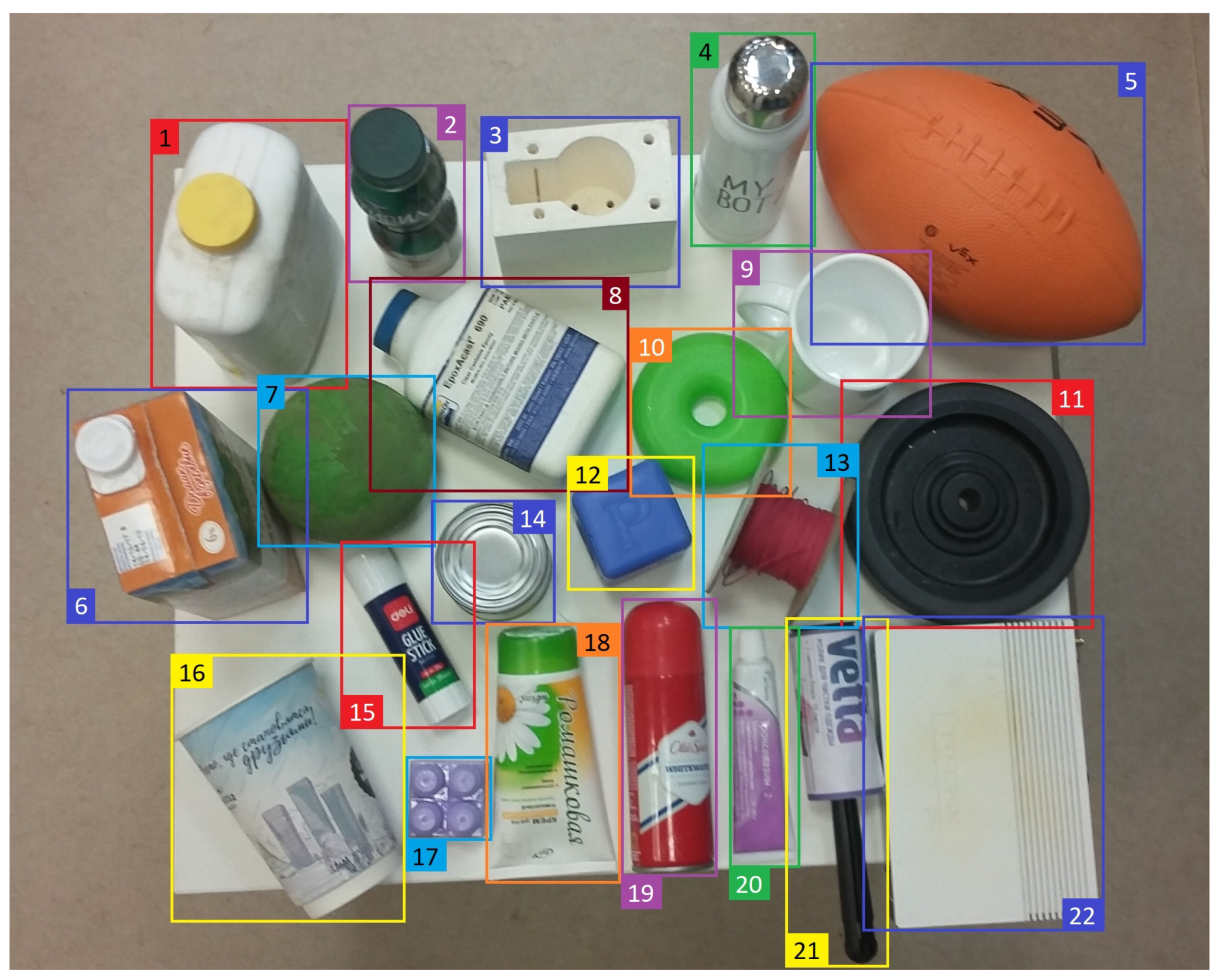
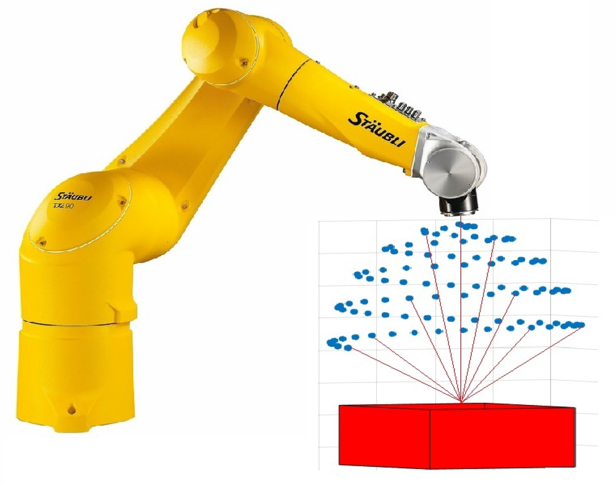
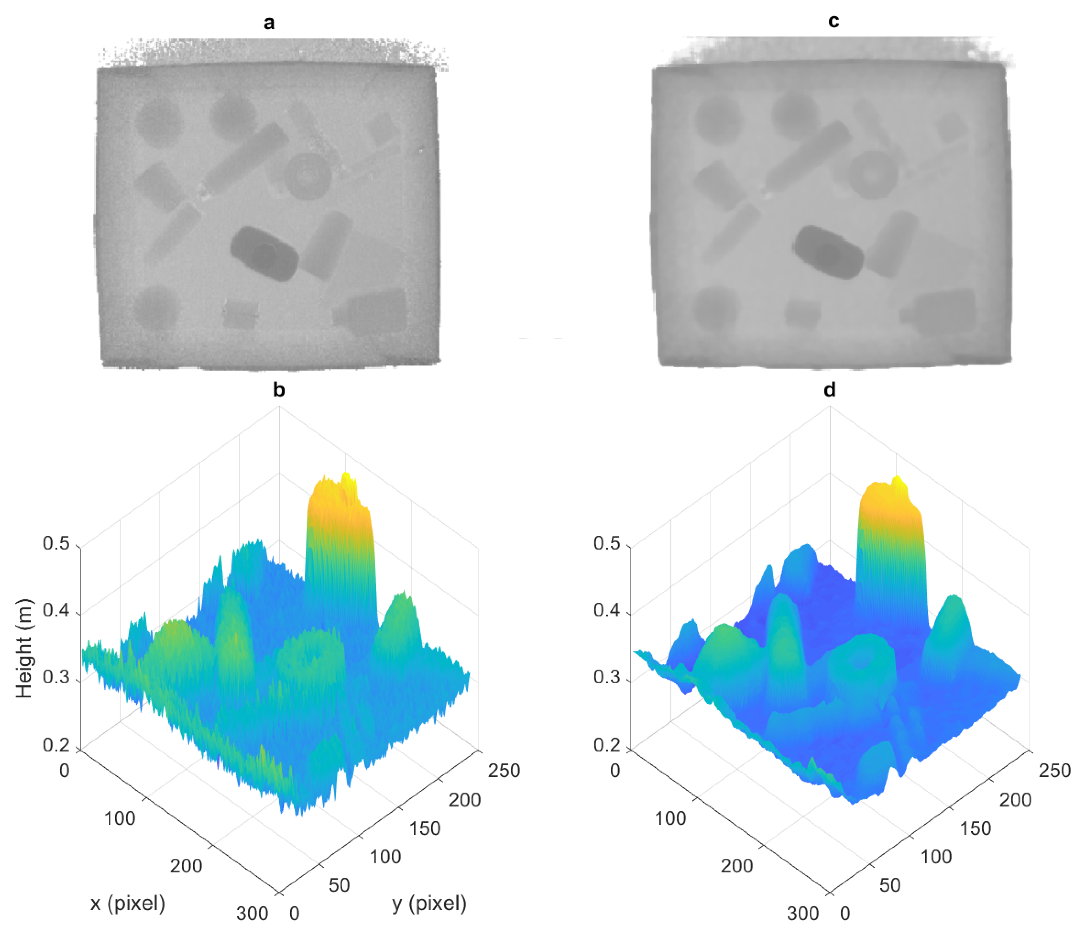
For our object recognition task, we selected objects (see Figure 2), which can be easily found and can fit into a regular delivery box with 0.5 m × 0.5 m × 0.1 m dimensions. To benchmark our object recognition framework, we generated a test dataset of real depth images. We conducted twenty experiments. During each experiment, 100 real-world depth and corresponding RGB images were acquired from different viewpoints using an RGB-D camera (SoftKinetic (Brussels, Belgium) DS325), which was attached to the end-effector of an industrial robot (Staubli (Pfäffikon, Switzerland) TX90XL). The robot followed a spiral trajectory, as shown in Figure 3, with the depth camera always pointing to the center of the box. Then, 16-bit depth images with 640 × 480 resolution were acquired at 30 frames per second (see Figure 4a). The number of objects, their positions and orientations inside the box were set randomly for each experiment. Consequently, 2000 real-world depth images were labeled manually using the software LabelImg. RGB images were utilized to simplify manual labeling. Pixel values in our depth images represent the distance from the camera to the objects in mm. Depth pixel values are saturated if the distance to an object is more than 1 m or less than 0.1 m (i.e., sensing range of the depth camera is between 0.1 m and 1 m).
Real-world depth images are noisy compared to our synthetic depth images. Thus, preprocessing of the real-world depth images is a necessary first step. Various filtering techniques are presented in the literature for depth images. Zhang et al. proposed asymmetric Gaussian filters to smooth abrupt changes in the object boundaries of depth images [38]. Averaging filters were utilized in [39,40]. In [41], a wavelet filter was applied to reduce the noisy features in the depth images. The application of the median filter for depth image preprocessing was presented in [42,43].
After experimenting with infinite impulse response, Gaussian, bilateral and median filters, we decided to use the median filter for its performance and computational efficiency. The median filter is a nonlinear spatial filter which finds the median of a neighborhood centered about a pixel (see Figure 4).

3.2. Synthetic Dataset Generation

We used Solidworks CAD software in order to create the 3D models of 22 objects replicating the shape and size of the original objects as much as possible. Standard Triangle Language (STL) files were generated from these 3D models using Blender (Amsterdam, Netherlands), an open-source 3D computer graphics software. Since Blender uses its own metric, all generated STL files were scaled such that one Blender unit (1 BU) corresponds to 0.1 m. Depth rendering capability of Blender was utilized to create the synthetic depth scenes. The Blender camera parameters were changed to match the real-world depth camera. The real-world and synthetic scenes have a similar camera position and orientation (see Figure 3). Similar to the real-world experiment, a virtual box was created for object placement. Our strategy for synthetic depth data generation consisted of three steps:
  • Synthesis of a realistic scene (i.e., the box with objects)
  • Generation of depth and object silhouette images
  • Generation of bounding boxes and occlusion refinement

3.2.1. Cluttered Scene Synthesis

We first imported the 3D model of the main box into the Blender as a rigid body. We chose the bounding box type as “mesh”, which allows the simulator to use the original shape of the object for physical simulation. Since the box is concave, the use of the other option (i.e., convex hull) would result in a rectangular prism not suitable for the task.
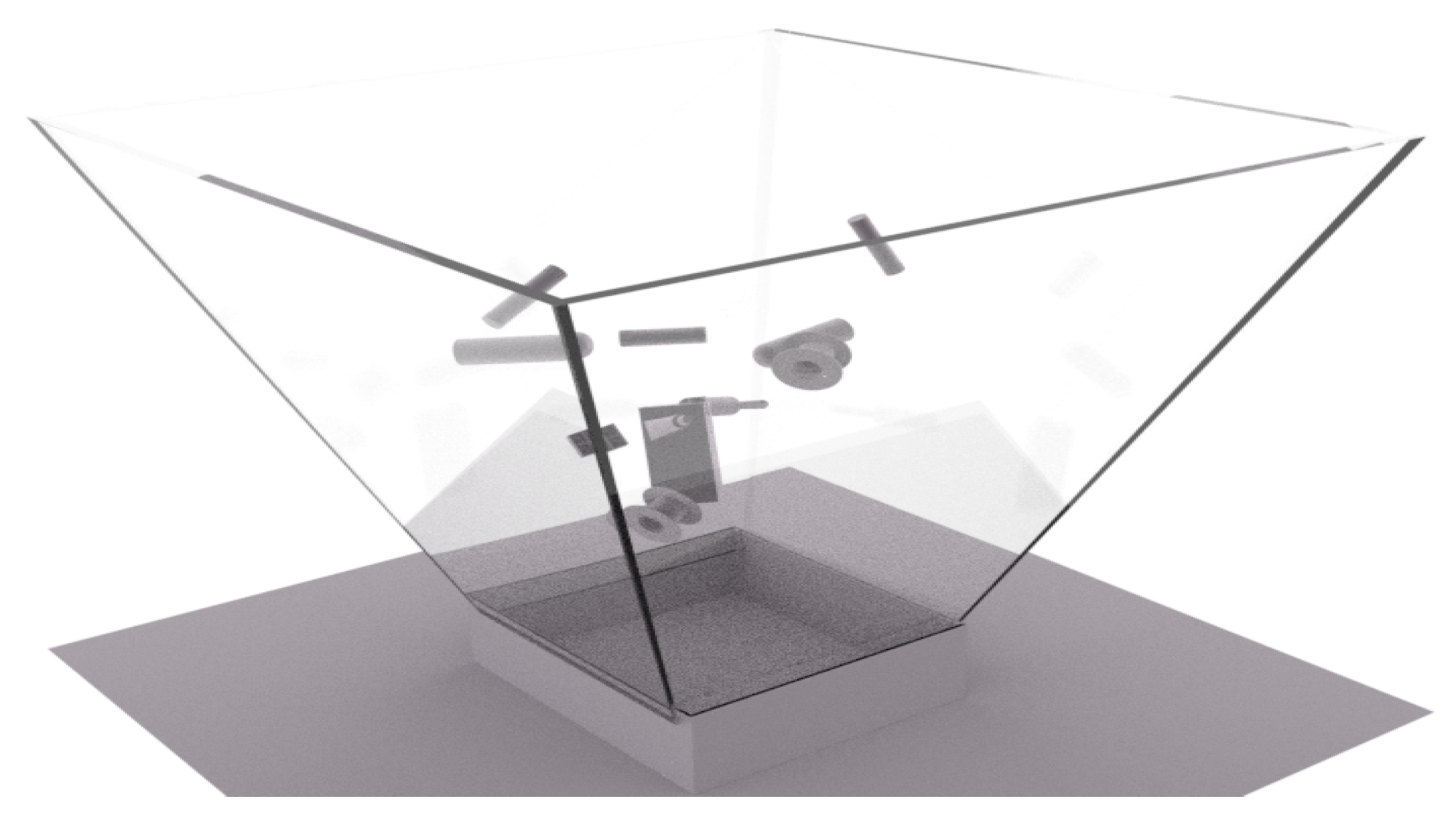
To create a physically-realistic box scene with multiple objects inside, we simulated the fall of these objects from a certain height into the box. Twenty-two objects were chosen with replacement from the original list of objects (i.e., some of the objects might be chosen more than once, and some of the objects might not be present in a scene.). These objects were randomly placed in a larger virtual box such that none of them intersect with another (see Figure 5). Then, they were released from their initial positions and fell into the box creating a realistic scene. A video provided as Supplementary Material shows the fall of the objects into the box.
In Blender, the process of saving information of a physical simulation is called “baking”. Baking of the objects for one physical simulation took between 2 and 15 s during which positions and orientations of each object were calculated for 250 frames (roughly corresponding to 8 s in simulation time). In most cases, this duration sufficed for objects to fall down and become stationary which was verified by visually monitoring the animation. However, some objects were still moving after landing on the surface due to properties such as friction, bounciness, damping, and collision margins. Therefore, we stopped the physical simulation after 250 frames to ensure the objects are stationary. Afterward, we started the rendering process, which takes around 0.5–0.8 s for each image. Parameters of both Blender and real-world cameras were 640 × 480 resolution, 16-bit depth levels, near clipping distance of 0.1 m, far clipping distance of 1 m and horizontal field of view of 74 degrees. The rendering consisted of the following steps:
  • Set the camera pose for the frame i.
  • Render the depth image for the frame i.
  • Generate n black and white (BW) object shape silhouettes for n objects within each frame i.

3.2.2. Generation of Depth and Object Silhouette Images

Once the physical simulation was completed, we generated two sets of images for 100 camera poses: (1) depth images; and (2) BW silhouette images. The silhouette images were used to detect the occlusions of the objects. To simplify the rendering process of the BW images, black diffuse material was assigned to an object while all other objects and the background were set to white. Thus, the output image consisted of only black pixels for the object seen from a specific camera pose and white elsewhere. To reduce the computation time, the resolution of these images was set to 20% of the original value (i.e., 128 × 96 pixels). Each object silhouette was saved as a bitmap format file with the filename consisting of the object name and the distance from the camera to the object center of mass. This process was repeated n times for n objects present in the scene. For each scene, there are 100 · n BW images containing information about object shapes for each 100 camera poses. In addition, for each scene, a text file with object pose information was created. It took between 0.2 and 0.5 s to generate the silhouette images for each scene.

3.2.3. Generation of Bounding Boxes and Occlusion Refinement

We considered an object as occluded if more than 70% of it was covered by other objects, including the main box walls. These occluded objects were not considered for object detection training. Axis-aligned bounding boxes were generated for each object, and the corresponding occlusion rate was calculated automatically using the silhouette images. Specifically, the bounding boxes were generated using Matlab R2017a from the silhouette images (see Figure 6). There were two cases when an object was not visible and should not be used for training a machine learning model:
  • More than 70% of the object is occluded.
  • The object is fully or mostly out of the camera’s view.
In the first case, to find the occluded objects, we used the following method. We sorted the BW silhouette images from nearest to the camera to farthest. As shown in Figure 6, the binary intersection between two consequent layers was found and recorded as the part of Layer 2 (farther object) occluded by Layer 1 (nearest objects). The percentage of the occluded area was computed. Afterward, the first layer was replaced by the union of Layers 1 and 2, and the same operation was repeated. Thus, the area of intersection of two layers showed the occlusion of the object on Layer 2 by an object or a set of objects on Layer 1. Using the aforementioned approach, the objects with more than 70% occlusion were found and removed from the text file containing the class labels for machine learning.
In Figure 6, the white rectangle on the bottom of the black and white image (new object silhouette) in Iteration 1 is the box wall. The green color indicates which part of the object is occluded. In Iteration 2, the object is fully occluded by nearest objects (i.e., main box wall). In Iteration 3, less than 28% is occluded. The main advantage of this method is that the exact shape of the object is used to compute the occlusion rate instead of using a rectangular bounding box.
In the second case, an object is fully or mostly out of the camera field of view. We handled this by excluding the objects whose bounding box is too small. Specifically, we determined the width, height and area thresholds for the bounding boxes of each object to exclude them from the list of visible objects. Objects whose bounding box dimensions were lower than the determined thresholds were considered as being not visible.

3.3. Comparison of Synthetic and Real-World Depth Images

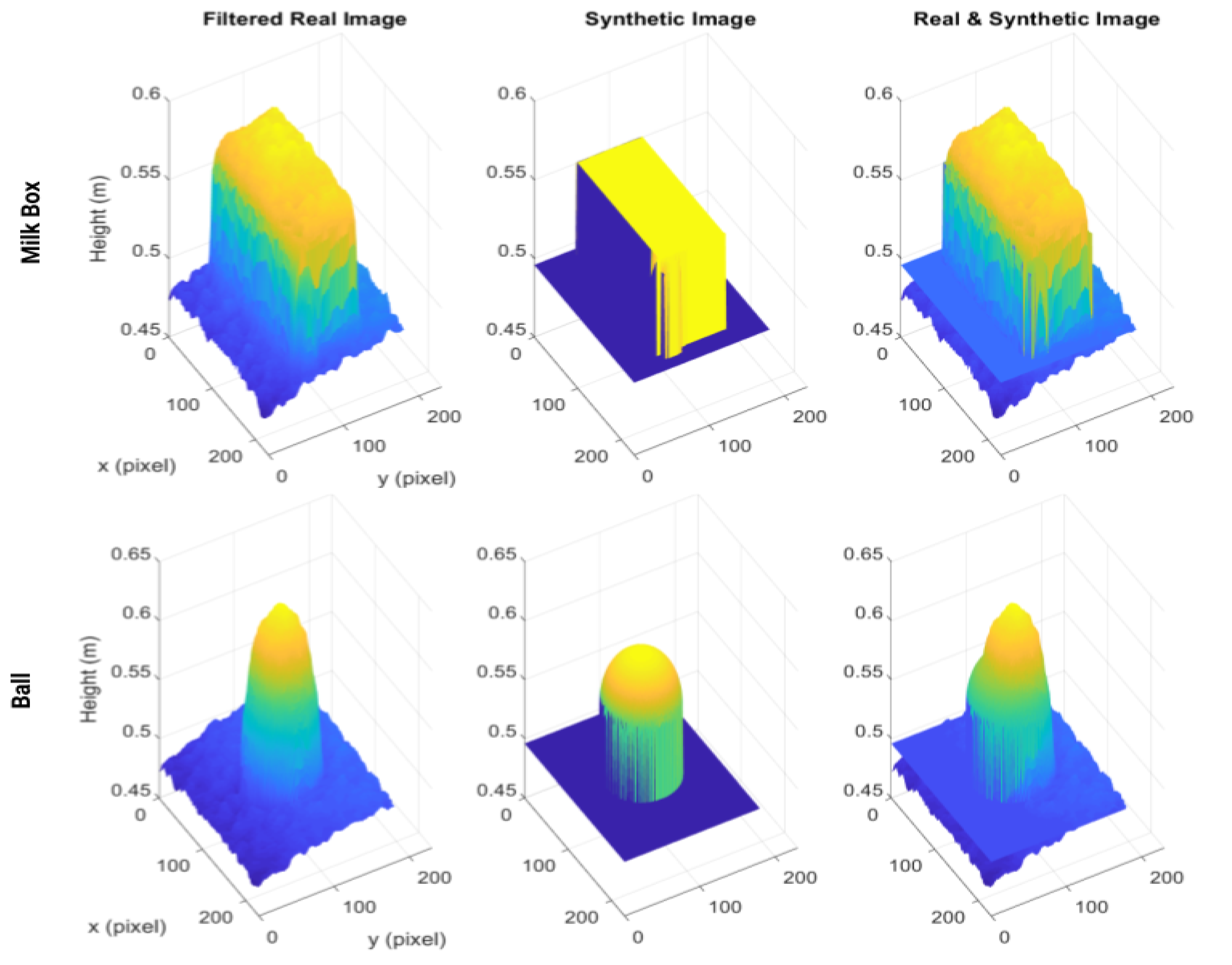
We generated the real-world dataset using the depth camera and smoothed using the median filter. Synthetic depth images were generated using the Blender software. To analyze the difference between synthetically generated and median filtered real-world depth images, we conducted the following experiment. An object was placed at the center of the box and depth images were acquired from a vertical distance of 50 cm. Similarly, the depth image of the object was generated synthetically by using the same camera parameters and pose (see Figure 7). To evaluate the pixel by pixel matching of these depth images, the root-mean-square errors (RMSEs) of the corresponding pixel values were found. The RMSE value for the milk box is 16 mm, and for the spherical ball is 21 mm.

3.4. Generation of Noise-Added Depth Images

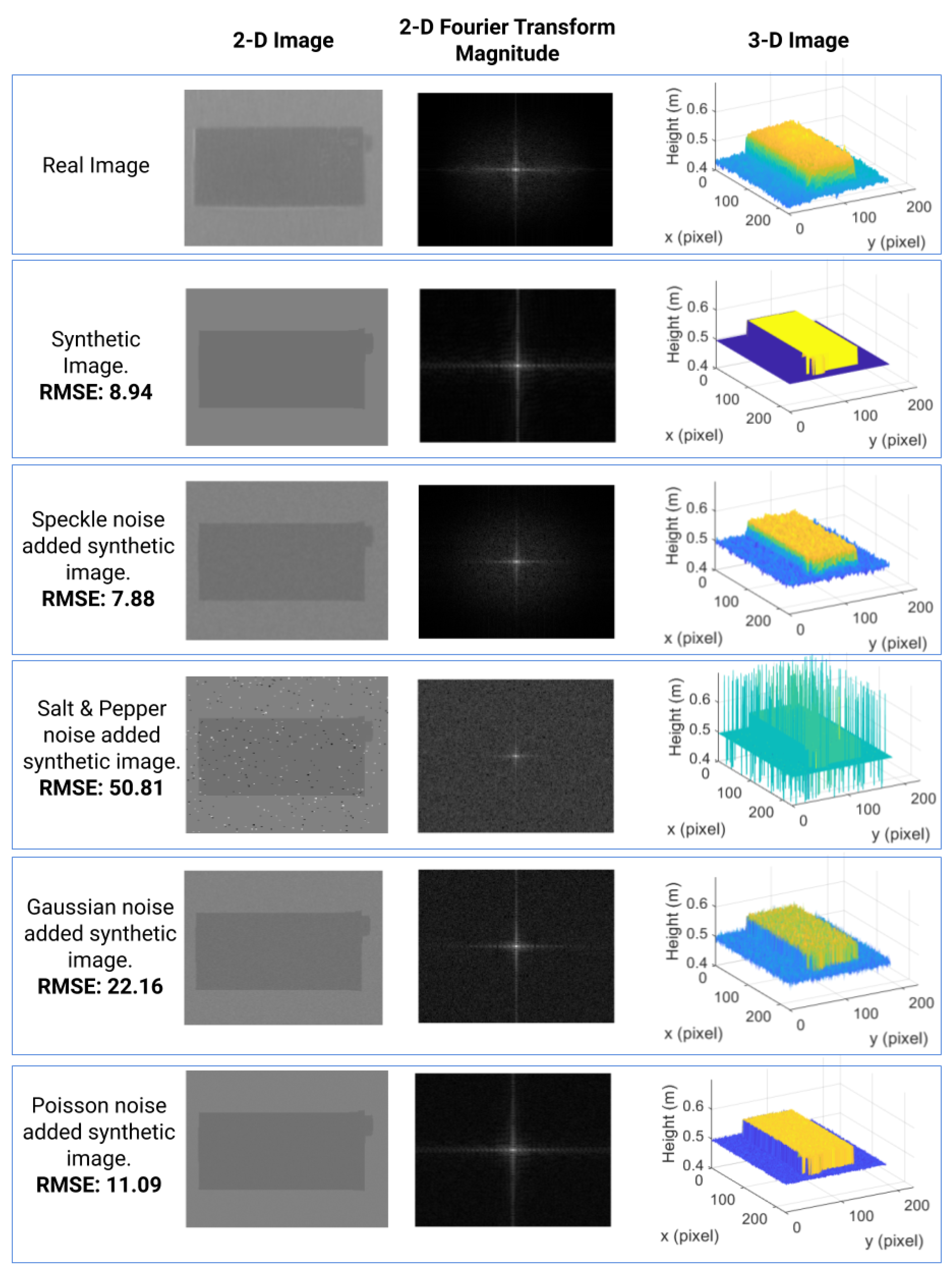
Most time-of-flight depth cameras suffer from random noise and bias. In our case, acquired real depth images also contain noise. On the other hand, synthetic images were generated without noise. One strategy to make the object detector robust against noise is to add similar noise to the synthetic depth images and train the network with these noisy images. Therefore, it is important to characterize the noise in real depth images. To investigate the noise properties, we acquired the depth image of the milk box and generated the synthetic depth image using the same camera pose, as shown in Figure 8. Then, we experimented by adding different types of noise such as Gaussian, salt and pepper, Poisson, and speckle noise to the synthetic image. Noise parameters such as mean, variance and density were found empirically because of the lack of a noiseless real-world depth image which could serve as ground truth. To analyze the noise-added synthetic images, we calculated the root-mean-squared error (RMSE) between the real and noise added synthetic images in the 2D frequency magnitude spectrums. In addition, we visualized the 2D Fourier transform and 3D plot of the real, synthetic and noise added synthetic images, as shown in Figure 8. After testing all mentioned noises, we found that the minimum RMSE was obtained for the speckle noise added image (Figure 8). In addition, the similarity between the real image and speckle noise-added synthetic image can be observed qualitatively in the frequency domain or in 3D plots (see Figure 8). Finally, 400,000 synthetic images with added speckle noise were generated. The variance of the speckle noise was randomly distributed between 0.001 and 0.002, and the standard deviation of the Gaussian filter was 0.9.

4. Deep Learning Model

4.1. Meta-Architectures: SSD, Faster R-CNN, and YOLO

Three notable DL meta-architectures developed for object recognition are SSD [8], Faster R-CNN [44] and YOLO [7]. SSD and Faster R-CNN use feature extractors as a base network for acquiring the dominant image features, while YOLO utilizes the single unified neural network for object detection. SSD takes the feature map from the feature extractor and adds multiple feature layers of different sizes. For each cell of these feature layers of size M × N × D , the anchor boxes of different scale and size are used to match them to ground truth boxes. For predicting the class scores and offsets of the anchor boxes, kernels of size 3 × 3 × D are used. All predictions are then sorted using non-maximum suppression, which excludes the predictions with low probability scores. Since SSD does not require region proposals, it is computationally efficient and faster than other architectures. However, SSD has lower accuracy because it reshapes the input to the fixed size of 300 × 300 or 600 × 600 resolution, which hinders the processing of large resolution images compared to other architectures as Faster R-CNN [44].
YOLO represents a single unified network for object detection. For YOLO, the image is first divided into N × N grid cells and then passed to the deep convolutional network, consisting of 24 convolutional layers and two fully connected layers. The outputs are sorted using non-maximum suppression. The limitations to its performance are related to the fact that for each cell in the grid only two bounding boxes are predicted. YOLO has difficulty in detecting small objects and objects that are close to each other [7]. Therefore, in a cluttered environment where many objects are occluded by each other, YOLO will have low performance.
In contrast to SSD and YOLO, Faster R-CNN uses the concept of region proposals, which are generated using the convolutional neural network called Region Proposal Network (RPN). RPN uses the sliding window with different anchor boxes over the feature map for computing the overlap of these anchors with the bounding boxes of objects (i.e., the ground truth). The number of the generated proposals is N = x · y · l / s , where x and y are the feature map size, l is the number of different anchor sizes, and s is the size of the stride. These proposals are sorted based on the prediction probability score. They are then used to crop the regions from the feature map, which are passed to the evaluation network for object classification and bounding box regression [9].

4.2. Feature Extractors

There is a number of feature extractor techniques, among which most popular are MobileNet, Resnet, and Inception [44]. MobileNeT uses the depth-wise separable convolutions, which are obtained by applying separate filters to each input channel (depth-wise convolution), and combining them with point-wise ( 1 × 1 ) convolution. In contrast, standard convolution applies one filter across all input channels [45]. The MobileNet architecture consists of 28 depth-wise and point-wise convolution layers, followed by average pooling and fully connected layers. Then, the Softmax layer is employed for classification. Even though deep neural networks usually have better performance with the increasing number of layers, there exists a degradation problem when the accuracy saturates and eventually decreases as the number of layers increases. To address this issue, residual networks (Resnet) implement identity mapping between the layers, which help to improve learning from the previous layers [46]. These residual connections are stacked together to form the Resnet network. Its implementations include Resnet-50, Resnet-101, and Resnet-152, having 50, 101, and 152 layers, respectively. The inception models are formed from the inception modules, which are generated by first computing 1 × 1 , 3 × 3 , and  5 × 5 max pooling convolutions and combining their different variations together before progressing to the next layer [47]. Recently, the inception modules were integrated with the residual connections by Szegedy et al. [47].
The performance of different DL models consisting of the described meta-architectures and feature extractors were analyzed in [44]. There is a trade-off between speed and accuracy of DL models. The fastest model was SSD with MobileNet, having the testing dataset mean average precision (mAP) of 18.8%, while most accurate was Faster R-CNN with Inception Resnet V2 feature extractor having 35.6% mAP. As we were mainly interested in the accuracy, we chose the latter for training.
We used a workstation (Intel Xeon E5-2620 CPU, 16 GB RAM) with a graphics accelerator (NVIDIA GeForce GTX 1080) to train our object recognition model using our synthetic dataset. The TensorFlow API for object detection has implementations of various feature extractors and meta-architectures. In addition, there are many pre-trained models on popular image datasets such as COCO, Kitti and Open Images [44]. However, all object detection models and checkpoints are implemented for 8-bit RGB images. Therefore, we modified the Faster R-CNN Inception Resnet V2 feature extractor to work for single-channel 16-bit depth images.

5. Experiments

We used two synthetic datasets for training the DL models. The first one consists of 800,000 clean synthetic depth images, and the second one consists of 400,000 clean synthetic and 400,000 noise-added synthetic depth images. Both models were trained from scratch using the initial learning rate of 0.01, decreasing 10 times at every epoch. In total, the models were trained for 4 epochs. The momentum was set to 0.9, and the batch size was set to 6 due to memory limitation. The number of region proposals was 300 and the output stride of 16 was chosen. The DL models were then tested on both synthetic and real depth images. The first testing dataset consists of 20,000 clean synthetic images (not included in the training dataset), while the second testing dataset consists of 2000 real-world depth images.

Accuracy Evaluation

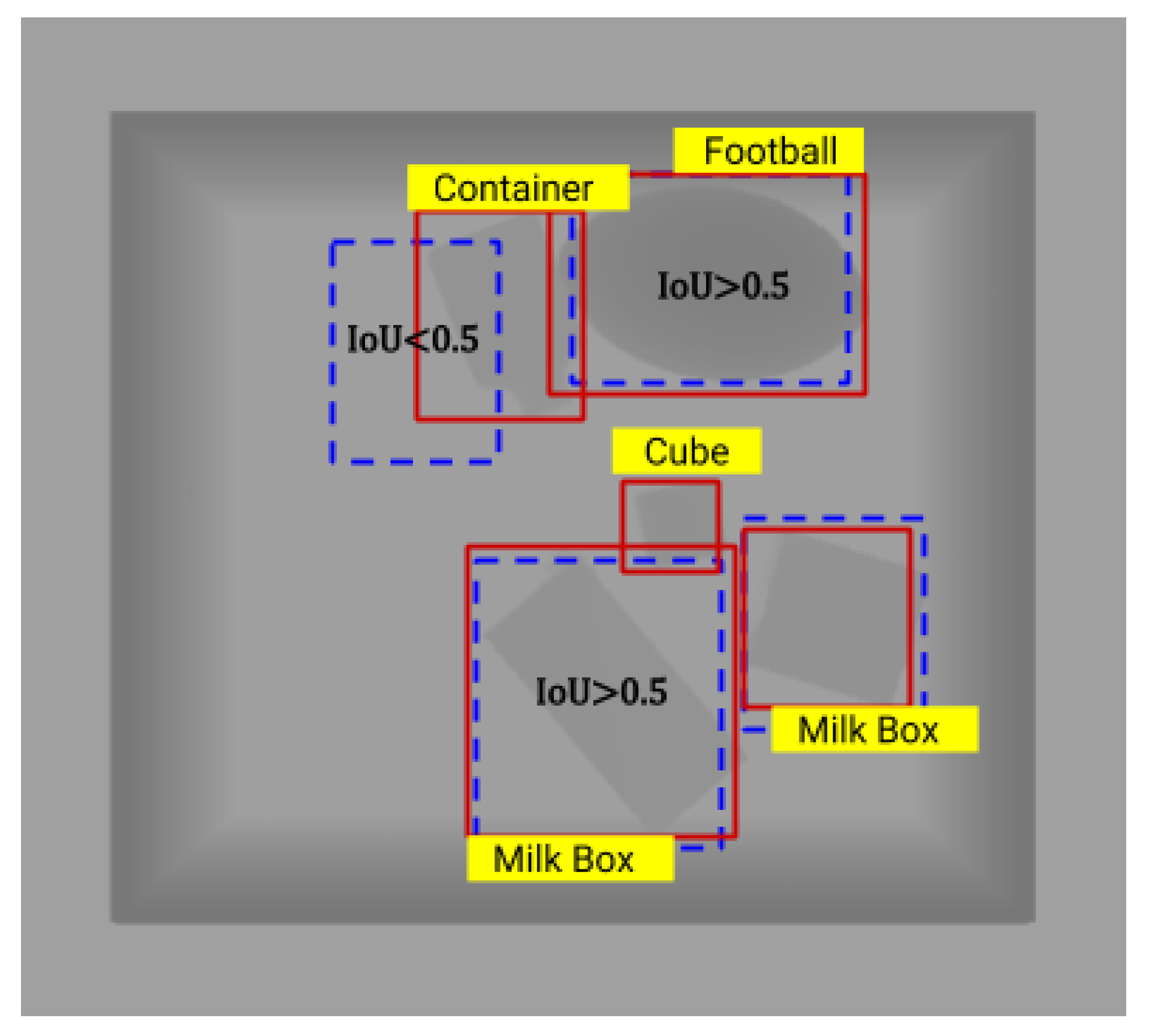
To benchmark the accuracy of our model, we used the intersection over union (IoU) metric [48]. Based on this metric, as shown in Figure 9, we considered a prediction as correct if the overlap ratio of the ground truth bounding box (solid red) and predicted one of the object (dashed blue) is more than the threshold value of 0.5. For example, the bounding box overlap ratios for the “Milk Box” and “Football” exceed 0.5 and these predictions are regarded as true positives (TP). In contrast, the overlap ratio for the “Container” is less than 0.5, and “3D Part” is predicted as “Milk Box”, so both are regarded as false positives (FP). In addition, the model prediction misses the “Cube” object which exists in the ground truth. Therefore, the “Cube” is counted as a false negative (FN).
Following these rules, we computed the accuracy of model predictions using the procedure presented in Algorithm 1. P is an output of our DL model for a testing image. It contains n predicted objects and their corresponding bounding boxes. G T is a ground truth information which contains m objects and their corresponding bounding boxes obtained from the real-world testing images via manual labeling. Initial values of T P , F P , and  F N were zero. Then, the predicted object names were compared with the object names in G T , and if the object existed in G T , the IoU score of their bounding boxes was calculated. If the IoU passed the threshold, T P was incremented by one. F P was obtained via subtracting T P from the number of objects in the GT image while F N was extracted via subtracting T P from the number of predicted objects. Afterward, we calculated the accuracy for one image as T P /( T P + F P + F N ). The average accuracy for the whole testing dataset was computed by finding the mean of the obtained accuracies for each image.
Algorithm 1 Accuracy evaluation routine.
  1: procedure Metric(P, G T )
  2:       T P 0
  3:       F P 0
  4:       F N 0
  5:      for i 1 , n do
  6:             for j 1 , m do
  7:             if c o m p a r e O b j N a m e s ( P ( i ) , G T ( j ) ) then
  8:                  I o U b o u n d i n g b o x ( P ( i ) G T ( j ) )
  9:                 if I o U 0.5 then
10:                      T P T P + 1
11:                 end if
12:             end if
13:          end for
14:      end for
15:       F P m T P
16:       F N n T P
17:       a c c u r a c y T P ÷ ( T P + F P + F N )
18:  end procedure

6. Results and Discussion

The deep object recognizer trained on synthetic clean images has 93.5% accuracy for synthetic testing and 40.96% for real-world testing datasets. Training with synthetic noise-added images improved the recognition accuracy to 96.1% and 46.3% for synthetic and real-world datasets, respectively, as presented in Table 1. The recognition accuracy per class (i.e., the ratio of correctly recognized objects to the total number of their appearance in the dataset) is presented in Table 2. In Table 2, we can see that recognition accuracy for real depth images increased for 14 out of 22 classes (shaded with green) after training with the noise-added dataset. However, we can also see a significant difference between the testing accuracies on the synthetic and real-world images. In addition, it can be noted that the recognition accuracy varies greatly for different object categories. Occlusion and different object properties such as size, shape similarity, and low/high reflectivity affect recognition accuracy.
For isolating the effects of the occlusion, the experiment for object recognition was conducted in an ideal environment. Specifically, each object was placed inside the box one by one and 100 images were taken from different camera poses. The classification results are summarized in Table 3 as a confusion matrix. The average recognition accuracy in the clean and unoccluded environment is 77%, which is significantly higher compared to the case with occlusion.
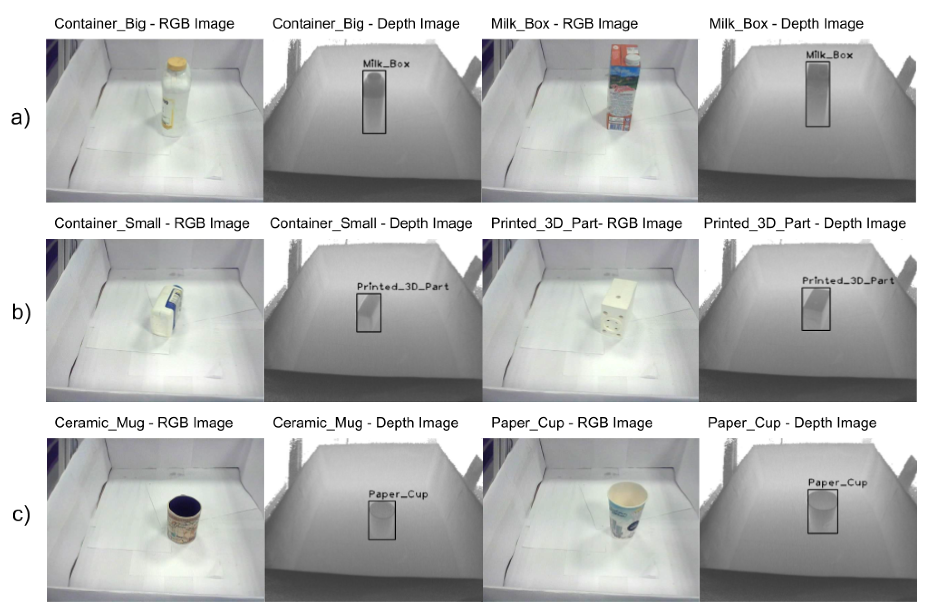
In Table 3, we can see that detection scores are high (above 85%) both for large objects (e.g., football, milk box, spherical ball, printed 3D part, paper cup, and cable reel) and small objects such as Lego brick, cube, ointment tube, and torus toy. However, other objects (e.g., cream tube, ceramic mug, small and big container) have lower accuracy due to shape similarity. The misclassifications of the objects due to shape similarity effects are illustrated in Figure 10. In the first row of Figure 10, the big container has a similar shape to the milk box. Therefore, DL model recognizes both of them as milk box. Similarly, in the second row, a small container is not correctly recognized as its shape is similar to that of a 3D printed part. In addition, ceramic mug, shown in the third row, is detected incorrectly as a paper cup, and it can be seen that their shapes are very similar from the specific perspective.
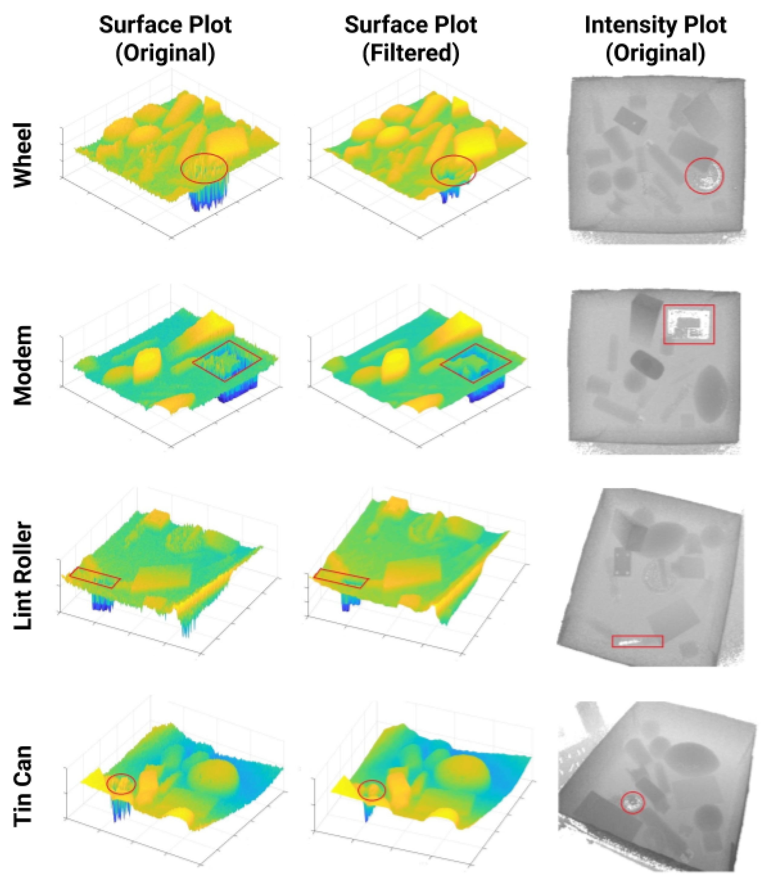
In addition, we can see that objects such as the wheel, yogurt bottle, lint roller, and tin can have low detection score because these objects have low or high reflectivity. Figure 11 shows real-world depth images containing reflective and black objects. The red circle in the first row and the red rectangles in the second and third rows in Figure 11 point out black objects (wheel, the dark side of the modem and lint roller), while the red circle in the fourth row points out a reflective object (tin can). Depending on the distance, the dark objects may seem to be farther away or closer because of non-linearities in the phase shift estimation [49]. Surface plots for objects before and after median filtering are presented in the first and second columns of Figure 11, respectively. The third column shows the corresponding original intensity plots. It can be seen that the dark and reflective objects have a substantial amount of white pixels at the maximum intensity value of 65,535. This means that depth information for the objects is not valid and cannot provide discriminative information for object recognition. This problem cannot be alleviated using median filter due to the large size of the saturated zones.
We can state that, in the ideal case, the main reason for misclassifications is the shape similarity. However, the objects with low or high reflectivity decrease the depth measurement quality and result in lower recognition accuracies. In general, both small and large objects not having these effects (i.e., shape similarity and low or high reflectivity) have higher recognition accuracies. If objects are placed in a cluttered environment, the performance of DL model recognition declines.
After analyzing the effects of the different object properties, we need to consider the effect of the occlusion. The occlusion effects influence the recognition slightly for the large objects which do not have shape similarities with other objects. For example, Table 2 shows that the detection scores for objects such as football, milk box, printed 3D part, spherical ball are high even with part of these objects occluded. However, the effect of the occlusion is detrimental for small objects, for which recognition accuracy decreases to less than 30%, while in the unoccluded environment small objects had a high accuracy of above 85%.
The advantages of our approach compared to the previous works are the following. The previous approaches of object recognition mainly use the RGB images [8,50,51,52]. However, generating large-scale dataset is costly as it requires the manualy labeling of millions of images. To tackle this issue, there have been some approaches of generating the synthetic RGB images, which mainly employed the following methods: cropping object images from available datasets and placing them on top of the random backgrounds [20,21] or RGB rendering of 3D CAD models with texture, color and visual information [5,19]. The mean average precision (mAP) of the object recognition is 24% for 55 object classes in [19] and 46% for 31 object classes in [5] compared to an average precision of 46.3% for 22 object classes in our work. These approaches have the following limitations. The former one is limited by the existing set of objects and is not robust to object recognition in cluttered and occluded environments (see Section 3.1 in [20]). The weakness of the latter one is related to the fact that object recognition with RGB images is vulnerable to the effects of the light, illumination and textual information. Therefore, it is challenging to create a dataset which takes all of these variations into account.
In addition, rendering of the depth images takes less time compared to the rendering of the RGB images. In our work, rendering of one depth image took around 0.8 s, while, in [53], rendering time of one high-quality RGB image was on average 14 s.
Thirdly, previous works related to object detection using depth images [17,54] have considered only a limited set of object types for testing: eight objects in [17] and six objects in [54]. The object detection accuracies of these approaches are 84.94% and 83% (mAP), respectively. However, these works also lack the analysis of the object recognizer performance in the case of the high or low reflectivity objects and objects with similar shapes or small sizes which can significantly influence the recognition accuracy. On the other hand, our work provides an extended analysis of the object recognition framework and effects of the different object properties such as size, shape similarity, and high/low reflectivity. In addition, our framework works in real-time (6 fps) using the depth camera even in a dark environment, which is the main weakness of the approaches based on RGB camera.
Our object recognition framework utilizing synthetic depth images and automatic labeling has some further limitations. In particular, we designed our detection system for 22 objects. Therefore, if the object set were changed, the model would need to be trained from scratch with a newly synthesized dataset. Another limitation is the resolution of the depth camera. The average noise of our depth camera was around 0.7 cm, which deteriorated the detection performance of small objects. We expect this problem to lessen due to the introduction of new depth cameras with better characteristics.

7. Conclusions

In this work, we present a DL-based object recognition framework using synthetic depth images. The models trained on clean and noise-added synthetic images were tested for object recognition of real-world depth images. The results of object recognition can be influenced by the effects of occlusion and other object properties. In an uncluttered environment, DL models trained with the synthetically generated depth data provide high accuracy for large and small objects. Shape similarity and high or low reflectivity of objects deteriorate the detection accuracy, with the latter having a more significant effect. The occlusion effect decreases object recognition accuracy significantly for small objects and objects having the shape similarities to other objects. The objects having low or high reflectivity are not suitable for object detection using the time-of-flight depth cameras, because depth information is not valid for object recognition. Our future work will entail the extension of the object set, use of different depth cameras and DL architectures. Our final aim is to utilize our framework in real-time object manipulation with an industrial robot.

Supplementary Materials

The following are available online at https://www.mdpi.com/2504-4990/1/3/51/s1, Video S1: Deep Learning Based Object Recognition Using Physically-Realistic Synthetic Depth Scenes.

Author Contributions

Conceptualization, H.A.V.; Data creation, A.O., D.F., Z.M. and A.K.; Project administration, H.A.V.; Software, D.B., A.Z. and A.K.; Supervision, H.A.V.; Writing—original draft, D.B., A.K. and Z.M.; and Writing—review and editing, D.B. and H.A.V.

Funding

This work was supported by the grant “Methods for Safe Human Robot Interaction with VIA Robots” from the Ministry of Education and Science of the Republic of Kazakhstan and by the Nazarbayev University Faculty Development Program grant “Hardware and Software Based Methods for Safe Human-Robot Interaction with Variable Impedance Robots”.

Conflicts of Interest

The authors declare no conflict of interest.

References

  1. Correll, N.; Bekris, K.E.; Berenson, D.; Brock, O.; Causo, A.; Hauser, K.; Okada, K.; Rodriguez, A.; Romano, J.M.; Wurman, P.R. Analysis and Observations From the First Amazon Picking Challenge. IEEE Trans. Autom. Sci. Eng. 2018, 15, 172–188. [Google Scholar] [CrossRef]
  2. Li, W.; Luo, Y.; Wang, P.; Qin, Z.; Zhou, H.; Qiao, H. Recent advances on application of deep learning for recovering object pose. In Proceedings of the IEEE International Conference on Robotics and Biomimetics (ROBIO), Qingdao, China, 3–7 December 2016; pp. 1273–1280. [Google Scholar] [CrossRef]
  3. LeCun, Y.; Bengio, Y.; Hinton, G. Deep learning. Nature 2015, 521, 436–444. [Google Scholar] [CrossRef] [PubMed]
  4. Gupta, S.; Arbeláez, P.; Girshick, R.; Malik, J. Aligning 3D models to RGB-D images of cluttered scenes. In Proceedings of the IEEE Conference on Computer Vision and Pattern Recognition (CVPR), Boston, MA, USA, 7–12 June 2015; pp. 4731–4740. [Google Scholar] [CrossRef]
  5. Peng, X.; Sun, B.; Ali, K.; Saenko, K. Learning deep object detectors from 3D models. In Proceedings of the IEEE International Conference on Computer Vision, Santiago, Chile, 7–13 December 2015; pp. 1278–1286. [Google Scholar]
  6. Girshick, R.; Donahue, J.; Darrell, T.; Malik, J. Rich feature hierarchies for accurate object detection and semantic segmentation. In Proceedings of the IEEE Conference on Computer Vision and Pattern Recognition (CVPR), Columbus, OH, USA, 23–28 June 2014; pp. 580–587. [Google Scholar]
  7. Redmon, J.; Divvala, S.; Girshick, R.; Farhadi, A. You only look once: Unified, real-time object detection. In Proceedings of the Conference on Computer Vision and Pattern Recognition (CVPR), Las Vegas, NV, USA, 27–30 June 2016; pp. 779–788. [Google Scholar]
  8. Liu, W.; Anguelov, D.; Erhan, D.; Szegedy, C.; Reed, S.; Fu, C.Y.; Berg, A.C. SSD: Single shot multibox detector. In Proceedings of the European Conference on Computer Vision, Amsterdam, The Netherlands, 8–16 October 2016; pp. 21–37. [Google Scholar]
  9. Ren, S.; He, K.; Girshick, R.; Sun, J. Faster R-CNN: Towards real-time object detection with region proposal networks. IEEE Trans. Pattern Anal. Mach. Intell. 2017, 1137–1149. [Google Scholar] [CrossRef] [PubMed]
  10. Krizhevsky, A.; Sutskever, I.; Hinton, G.E. ImageNet classification with deep convolutional neural networks. In Proceedings of the Advances in Neural Information Processing Systems, Lake Tahoe, NV, USA, 3–6 December 2012; pp. 1097–1105. [Google Scholar]
  11. Carlucci, F.M.; Russo, P.; Caputo, B. A deep representation for depth images from synthetic data. In Proceedings of the IEEE International Conference on Robotics and Automation (ICRA), Singapore, 29 May–3 June 2017; pp. 1362–1369. [Google Scholar]
  12. Zhang, Y.; Song, S.; Yumer, E.; Savva, M.; Lee, J.Y.; Jin, H.; Funkhouser, T. Physically-based rendering for indoor scene understanding using convolutional neural networks. In Proceedings of the IEEE Conference on Computer Vision and Pattern Recognition (CVPR), Honolulu, HI, USA, 21–26 July 2017; pp. 5057–5065. [Google Scholar]
  13. Mitash, C.; Bekris, K.E.; Boularias, A. A self-supervised learning system for object detection using physics simulation and multi-view pose estimation. In Proceedings of the IEEE/RSJ International Conference on Intelligent Robots and Systems (IROS), Vancouver, BC, Canada, 24–28 September 2017; pp. 545–551. [Google Scholar]
  14. Ben-David, S.; Blitzer, J.; Crammer, K.; Pereira, F. Analysis of representations for domain adaptation. In Proceedings of the Advances in Neural Information Processing Systems, Vancouver, BC, Canada, 3–6 December 2007; pp. 137–144. [Google Scholar]
  15. Ganin, Y.; Ustinova, E.; Ajakan, H.; Germain, P.; Larochelle, H.; Laviolette, F.; Marchand, M.; Lempitsky, V. Domain-adversarial training of neural networks. J. Mach. Learn. Res. 2016, 17, 1–35. [Google Scholar]
  16. Hinterstoisser, S.; Lepetit, V.; Wohlhart, P.; Konolige, K. On Pre-trained Image Features and Synthetic Images for Deep Learning. In Proceedings of the ECCV Workshops, Munich, Germany, 8–14 September 2018; pp. 682–697. [Google Scholar]
  17. Mithun, N.C.; Munir, S.; Guo, K.; Shelton, C. ODDS: Real-Time Object Detection Using Depth Sensors on Embedded GPUs. In Proceedings of the 2018 17th ACM/IEEE International Conference on Information Processing in Sensor Networks (IPSN), Porto, Portugal, 11–13 April 2018; pp. 230–241. [Google Scholar] [CrossRef]
  18. Pinto, N.; Barhomi, Y.; Cox, D.D.; DiCarlo, J.J. Comparing state-of-the-art visual features on invariant object recognition tasks. In Proceedings of the IEEE Workshop on Applications of Computer Vision (WACV), Kona, HI, USA, 5–7 January 2011; pp. 463–470. [Google Scholar]
  19. Rajpura, P.S.; Hegde, R.S.; Bojinov, H. Object Detection Using Deep CNNs Trained on Synthetic Images. arXiv, 2017; arXiv:1706.06782. [Google Scholar]
  20. Georgakis, G.; Mousavian, A.; Berg, A.C.; Kosecka, J. Synthesizing Training Data for Object Detection in Indoor Scenes. arXiv, 2017; arXiv:1702.07836. [Google Scholar]
  21. Dwibedi, D.; Misra, I.; Hebert, M. Cut, Paste and Learn: Surprisingly Easy Synthesis for Instance Detection. In Proceedings of the IEEE International Conference on Computer Vision 2017, Venice, Italy, 22–29 October 2017. [Google Scholar]
  22. Lai, K.; Bo, L.; Ren, X.; Fox, D. A large-scale hierarchical multi-view RGB-D object dataset. In Proceedings of the IEEE International Conference on Robotics and Automation (ICRA), Shanghai, China, 9–13 May 2011; pp. 1817–1824. [Google Scholar]
  23. Socher, R.; Huval, B.; Bath, B.; Manning, C.D.; Ng, A.Y. Convolutional-recursive deep learning for 3D object classification. In Proceedings of the Advances in Neural Information Processing Systems, Lake Tahoe, NV, USA, 3–6 December 2012; pp. 656–664. [Google Scholar]
  24. Schwarz, M.; Milan, A.; Periyasamy, A.S.; Behnke, S. RGB-D object detection and semantic segmentation for autonomous manipulation in clutter. Int. J. Robot. Res. 2018, 37, 437–451. [Google Scholar] [CrossRef]
  25. Newcombe, R.A.; Izadi, S.; Hilliges, O.; Molyneaux, D.; Kim, D.; Davison, A.J.; Kohi, P.; Shotton, J.; Hodges, S.; Fitzgibbon, A. KinectFusion: Real-time dense surface mapping and tracking. In Proceedings of the IEEE International Symposium on Mixed and Augmented Reality (ISMAR), Basel, Switzerland, 26–29 October 2011; pp. 127–136. [Google Scholar]
  26. Izadi, S.; Kim, D.; Hilliges, O.; Molyneaux, D.; Newcombe, R.; Kohli, P.; Shotton, J.; Hodges, S.; Freeman, D.; Davison, A.; et al. KinectFusion: Real-time 3D reconstruction and interaction using a moving depth camera. In Proceedings of the ACM Symposium on User Interface Software and Technology, Santa Barbara, CA, USA, 16–19 October 2011; pp. 559–568. [Google Scholar]
  27. Shotton, J.; Fitzgibbon, A.; Cook, M.; Sharp, T.; Finocchio, M.; Moore, R.; Kipman, A.; Blake, A. Real-time human pose recognition in parts from single depth images. In Proceedings of the IEEE Conference on Computer Vision and Pattern Recognition (CVPR), Washington, DC, USA, 20–25 June 2011; pp. 1297–1304. [Google Scholar]
  28. Biswas, J.; Veloso, M. Depth camera based indoor mobile robot localization and navigation. In Proceedings of the IEEE International Conference on Robotics and Automation (ICRA), St Paul, MN, USA, 14–18 May 2012; pp. 1697–1702. [Google Scholar]
  29. Maier, D.; Hornung, A.; Bennewitz, M. Real-time navigation in 3D environments based on depth camera data. In Proceedings of the IEEE-RAS International Conference on Humanoid Robots, Osaka, Japan, 29 November–1 December 2012; pp. 692–697. [Google Scholar]
  30. Saudabayev, A.; Kungozhin, F.; Nurseitov, D.; Varol, H.A. Locomotion strategy selection for a hybrid mobile robot using time of flight depth sensor. J. Sens. 2015, 2015, 425732. [Google Scholar] [CrossRef]
  31. Massalin, Y.; Abdrakhmanova, M.; Varol, H.A. User-Independent Intent Recognition for Lower Limb Prostheses Using Depth Sensing. IEEE Trans. Biomed. Eng. 2018, 65, 1759–1770. [Google Scholar] [PubMed]
  32. Saudabayev, A.; Rysbek, Z.; Khassenova, R.; Varol, H.A. Human grasping database for activities of daily living with depth, color and kinematic data streams. Sci. Data 2018, 5, 180101. [Google Scholar] [CrossRef] [PubMed]
  33. Koenig, N.P.; Howard, A. Design and use paradigms for Gazebo, an open-source multi-robot simulator. In Proceedings of the IEEE/RSJ International Conference on Intelligent Robots and Systems (IROS), Sendai, Japan, 28 September–2 October 2004; Volume 4, pp. 2149–2154. [Google Scholar]
  34. Gschwandtner, M.; Kwitt, R.; Uhl, A.; Pree, W. BlenSor: Blender Sensor Simulation Toolbox. In Proceedings of the International Symposium on Visual Computing, Las Vegas, NV, USA, 26–28 September 2011; pp. 199–208. [Google Scholar]
  35. Liebelt, J.; Schmid, C. Multi-view object class detection with a 3D geometric model. In Proceedings of the IEEE Conference on Computer Vision and Pattern Recognition (CVPR), San Francisco, CA, USA, 13–18 June 2010; pp. 1688–1695. [Google Scholar]
  36. Gupta, A.; Vedaldi, A.; Zisserman, A. Synthetic data for text localisation in natural images. In Proceedings of the IEEE Conference on Computer Vision and Pattern Recognition (CVPR), Las Vegas, NV, USA, 27–30 June 2016; pp. 2315–2324. [Google Scholar]
  37. Wanner, S.; Goldluecke, B. Globally consistent depth labeling of 4D light fields. In Proceedings of the IEEE Conference on Computer Vision and Pattern Recognition (CVPR), Providence, RI, USA, 18–20 June 2012; pp. 41–48. [Google Scholar]
  38. Zhang, L.; Tam, W.J. Stereoscopic image generation based on depth images for 3D TV. IEEE Trans. Broadcast. 2005, 51, 191–199. [Google Scholar] [CrossRef]
  39. Cheng, C.M.; Lin, S.J.; Lai, S.H.; Yang, J.C. Improved novel view synthesis from depth image with large baseline. In Proceedings of the International Conference on Pattern Recognition (ICPR), Tampa, FL, USA, 8–11 December 2008; pp. 1–4. [Google Scholar]
  40. Park, Y.K.; Jung, K.; Oh, Y.; Lee, S.; Kim, J.K.; Lee, G.; Lee, H.; Yun, K.; Hur, N.; Kim, J. Depth-image-based rendering for 3DTV service over T-DMB. Signal Process. Image Commun. 2009, 24, 122–136. [Google Scholar] [CrossRef]
  41. Forster, B.; Van De Ville, D.; Berent, J.; Sage, D.; Unser, M. Complex wavelets for extended depth-of-field: A new method for the fusion of multichannel microscopy images. Microsc. Res. Tech. 2004, 65, 33–42. [Google Scholar] [CrossRef] [PubMed] [Green Version]
  42. Weiss, B. Fast median and bilateral filtering. ACM Trans. Graph. (TOG) 2006, 25, 519–526. [Google Scholar] [CrossRef]
  43. Ibarra-Castanedo, C.; Gonzalez, D.; Klein, M.; Pilla, M.; Vallerand, S.; Maldague, X. Infrared image processing and data analysis. Infrared Phys. Technol. 2004, 46, 75–83. [Google Scholar] [CrossRef]
  44. Huang, J.; Rathod, V.; Sun, C.; Zhu, M.; Balan, A.K.; Fathi, A.; Fischer, I.; Wojna, Z.; Song, Y.; Guadarrama, S.; et al. Speed/Accuracy Trade-Offs for Modern Convolutional Object Detectors. In Proceedings of the IEEE Conference on Computer Vision and Pattern Recognition (CVPR), Honolulu, HI, USA, 20–25 June 2017; pp. 3296–3297. [Google Scholar]
  45. Howard, A.G.; Zhu, M.; Chen, B.; Kalenichenko, D.; Wang, W.; Weyand, T.; Andreetto, M.; Adam, H. MobileNets: Efficient Convolutional Neural Networks for Mobile Vision Applications. arXiv, 2017; arXiv:1704.04861. [Google Scholar]
  46. He, K.; Zhang, X.; Ren, S.; Sun, J. Deep Residual Learning for Image Recognition. In Proceedings of the IEEE Conference on Computer Vision and Pattern Recognition (CVPR), Las Vegas, NV, USA, 27–30 June 2016; pp. 770–778. [Google Scholar] [CrossRef]
  47. Szegedy, C.; Ioffe, S.; Vanhoucke, V. Inception-v4, Inception-ResNet and the Impact of Residual Connections on Learning. In Proceedings of the AAAI Conference on Artificial Intelligence, San Francisco, CA, USA, 4–9 February 2017. [Google Scholar]
  48. Everingham, M.; Gool, L.; Williams, C.K.; Winn, J.; Zisserman, A. The Pascal Visual Object Classes (VOC) Challenge. Int. J. Comput. Vis. 2010, 88, 303–338. [Google Scholar] [CrossRef]
  49. Falie, D.; Buzuloiu, V. Noise Characteristics of 3D Time-of-Flight Cameras. In Proceedings of the International Symposium on Signals, Circuits and Systems, Iasi, Romania, 13–14 July 2007; Volume 1, pp. 1–4. [Google Scholar]
  50. Krizhevsky, A.; Sutskever, I.; Hinton, G.E. ImageNet Classification with Deep Convolutional Neural Networks. Neural Inf. Process. Syst. 2012, 25. [Google Scholar] [CrossRef]
  51. Szegedy, C.; Liu, W.; Jia, Y.; Sermanet, P.; Reed, S.; Anguelov, D.; Erhan, D.; Vanhoucke, V.; Rabinovich, A. Going deeper with convolutions. In Proceedings of the 2015 IEEE Conference on Computer Vision and Pattern Recognition (CVPR), Boston, MA, USA, 7–12 June 2015; pp. 1–9. [Google Scholar] [CrossRef]
  52. Ren, S.; He, K.; Girshick, R.; Sun, J. Faster R-CNN: Towards real-time object detection with region proposal networks. In Advances in Neural Information Processing Systems, Proceedings of the 29th Annual Conference on Neural Information Processing Systems 2015, Montreal, QC, Canada, 7–12 December 2015; Neural Information Processing Systems Foundation, Inc. (NIPS): La Jolla, CA, USA; pp. 91–99.
  53. McCormac, J.; Handa, A.; Leutenegger, S.; Davison, A.J. SceneNet RGB-D: Can 5M Synthetic Images Beat Generic ImageNet Pre-training on Indoor Segmentation? In Proceedings of the 2017 IEEE International Conference on Computer Vision (ICCV), Venice, Italy, 22–29 October 2017; pp. 2697–2706. [Google Scholar]
  54. Eitel, A.; Springenberg, J.T.; Spinello, L.; Riedmiller, M.; Burgard, W. Multimodal deep learning for robust RGB-D object recognition. In Proceedings of the 2015 IEEE/RSJ International Conference on Intelligent Robots and Systems (IROS), Hamburg, Germany, 28 September–2 October 2015; pp. 681–687. [Google Scholar] [CrossRef]
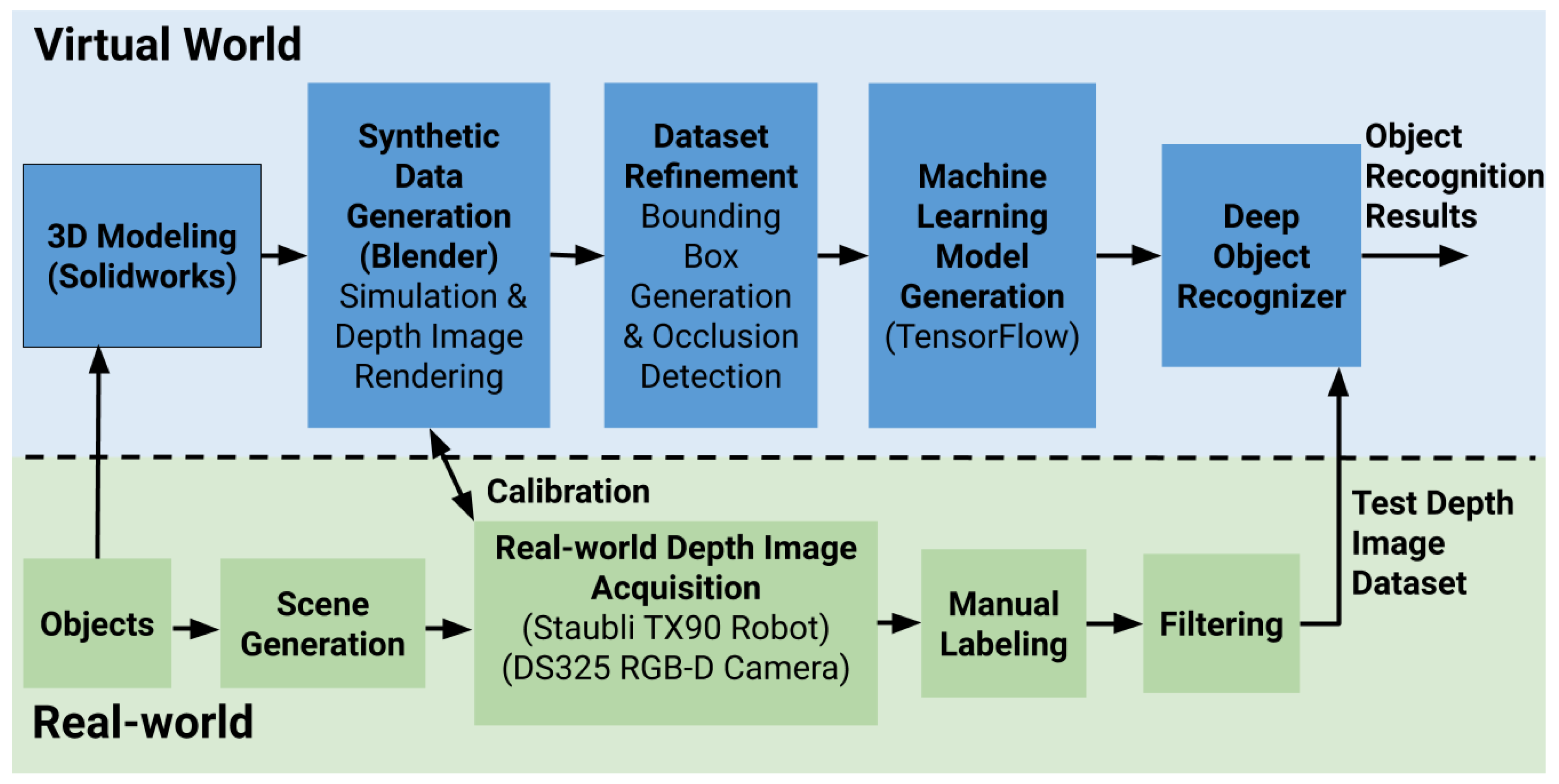
Figure 1. Block diagram of the depth-image-based object detection.
Make 01 00051 g001
Figure 2. Twenty-two objects chosen for the recognition task: (1) Container_Big; (2) Yogurt_Bottle; (3) Printed_3D_Part; (4) Thermos; (5) Football; (6) Milk_Box; (7) Spherical_Ball; (8) Container_Small; (9) Ceramic_Mug; (10) Torus_Toy; (11) Wheel; (12) Cube; (13) Cable_Reel; (14) Tin_Can; (15) Glue_Stick; (16) Paper_Cup; (17) Lego_Brick; (18) Cream_Tube; (19) Deodorant_Bottle; (20) Ointment_Tube; (21) Lint_Roller; and (22) Modem.
Make 01 00051 g002
Figure 3. Different RGB-D camera poses for real-world dataset generation.
Make 01 00051 g003
Figure 4. Raw depth image (a,b) and depth image median filtered with 9 × 9 kernel size (c,d). 2D figures (upper row) show the depth as grayscale intensity. 3D figures (bottom row) show the depth as z-axis value.
Make 01 00051 g004
Figure 5. Objects falling through the funnel into the main box during physical simulation to create a physically-realistic cluttered depth scene.
Make 01 00051 g005
Figure 6. Visualization of multiple mask layers used for occlusion estimation. Green region illustrates the part of the object occluded by the nearer objects.
Make 01 00051 g006
Figure 7. 3D comparison of the real and synthetic images.
Make 01 00051 g007
Figure 8. Figures of the real, synthetic and different types of noise-added synthetic images in 2D, Fourier domain and 3D.
Make 01 00051 g008
Figure 9. Illustration of the IoU metric.
Make 01 00051 g009
Figure 10. Visualization of the misclassification due to shape similarity: (a) the Container_Big is misclassified as a Milk_Box; (b) the Container_Small is misclassified as a Printed_3D_Part; and (c) the Ceramic_Mug is misclassified as a Paper_Cup.
Make 01 00051 g010
Figure 11. Reflective and black objects.
Make 01 00051 g011
Table 1. Object recognition performance comparison of DL models.
ModelsTesting Set
Synthetic Clean ImagesReal-World Images
Model 1 (trained with synthetic clean images)93.5%40.96%
Model 2 (trained with synthetic noise-added images)96.1%46.3
Table 2. Average object recognition accuracy (%) per class. Recognition accuracy after training with noise-added images increases in 14 out of 22 objects (green shaded cells). Dark and reflective objects are shaded with cyan. Small objects are shaded with red.
Model 1Model 2
ObjectsTesting Set: Synthetic Clean ImagesTesting Set: Real-World ImagesTesting Set: Synthetic Clean ImagesTesting Set: Real-World Images
Football99.9891.3799.9397.86
Milk_Box96.3690.0697.4493.52
Printed_3D_Part98.5476.8598.5888.89
Thermos97.5380.1296.6078.84
Spherical_Ball99.6777.8799.5877.67
Container_Big97.8365.1298.2475.48
Modem96.9671.5897.6867.77
Container_Small96.7363.3597.8361.10
Cable_Reel98.6954.6398.2956.63
Ceramic_Mug96.3351.2396.8955.75
Paper_Cup98.3341.8898.6254.86
Cube95.6043.8495.7854.20
Tin_Can94.4838.4796.2841.57
Cream_Tube91.3424.8894.5736.50
Lego_Brick84.5345.3889.0131.06
Lint_Roller92.0618.7191.6227.22
Ointment_Tube85.2628.4884.0624.09
Torus_Toy96.6721.8296.7420.10
Deodorant_Bottle95.5248.9195.4320.09
Yogurt_Bottle95.7211.3096.7919.94
Glue_Stick88.9012.5288.0919.73
Wheel98.7210.3298.4713.44
Table 3. Confusion matrix for object recognition for a single unoccluded object in the box. Correct recognitions are shaded with green. Dark and reflective objects are shaded with cyan. Small objects are shaded with red.
Predicted Classes
FootballMilk_BoxPrinted_3D_PartThermosSpherical_BallContainer_BigModemContainer_SmallCable_ReelCeramic_MugPaper_CupCubeTin_CanCream_TubeLego_BrickLint_RollerOintment_TubeTorus_ToyDeodorant_BottleYogurt_BottleGlue_StickWheel
Actual classesFootball100000000000000000000000
Milk_Box010000000000000000000000
Printed_3D_Part00930007000000000000000
Thermos06078008000000800000000
Spherical_Ball000010000000000000000000
Container_Big012000826000000000000000
Modem00400083005000080000000
Container_Small002300017600000000000000
Cable_Reel00000000880062040000000
Ceramic_Mug000000000831700000000000
Paper_Cup00400002009000400000000
Cube00000000000940060000000
Tin_Can0000000001408680100000000
Cream_Tube0020000000100075001300000
Lego_Brick000000000000001000000000
Lint_Roller000000000000000326000620
Ointment_Tube000000000000000087000130
Torus_Toy000000000000000001000000
Deodorant_Bottle00016000000000137650411200
Yogurt_Bottle00080000000001016812004600
Glue_Stick0000000000000401227000570
Wheel00800060030000024010000022