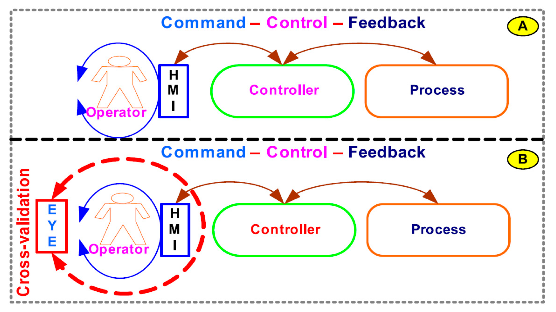
Figure 1.
Architecture of: (A) conventional operator-based command–control–feedback process systems; (B) expert supervisory system (EYE)-on-human–machine interface (HMI) adds cross-validation to operator command–control–feedback process systems.
Figure 1.
Architecture of: (A) conventional operator-based command–control–feedback process systems; (B) expert supervisory system (EYE)-on-human–machine interface (HMI) adds cross-validation to operator command–control–feedback process systems.
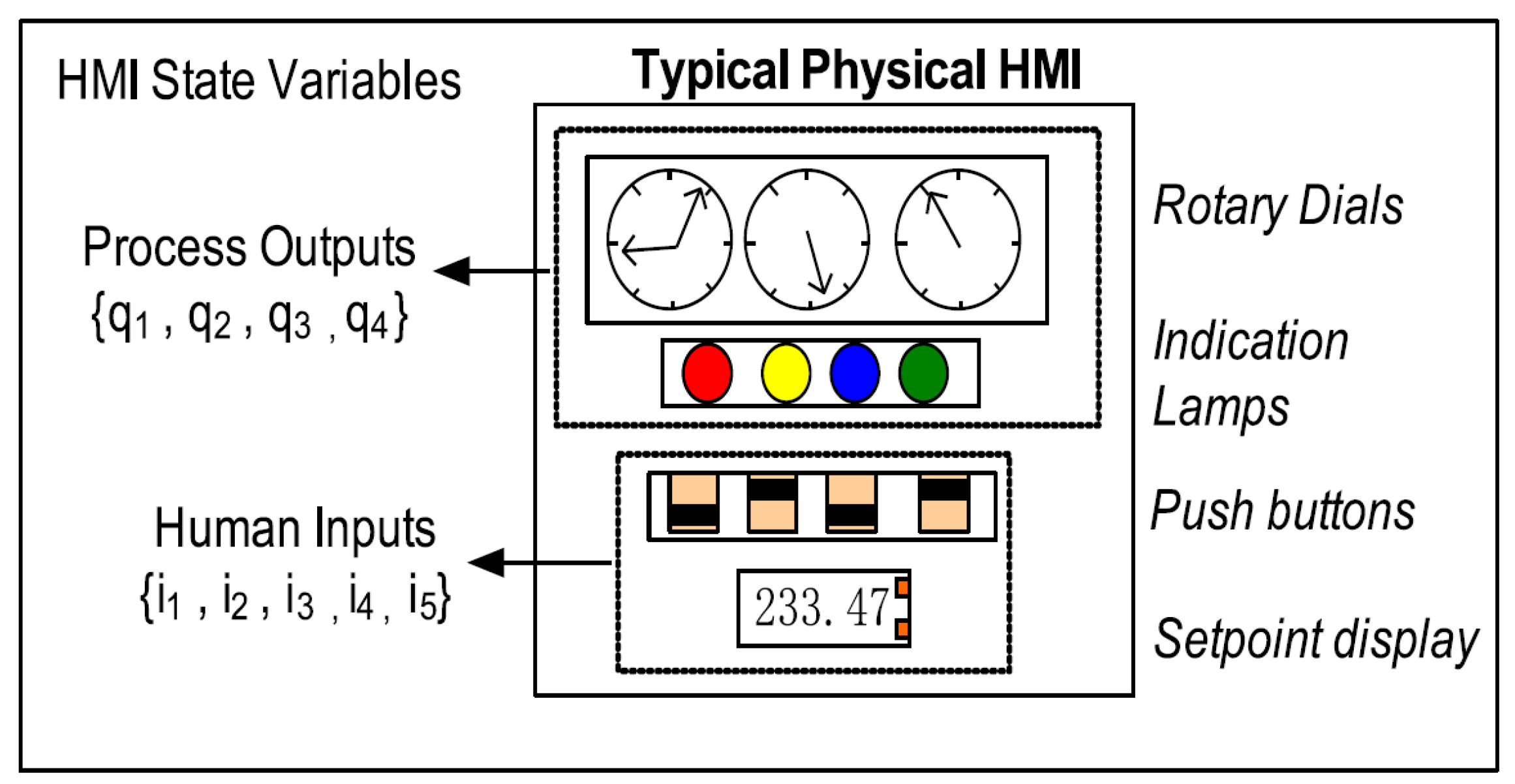
Figure 2.
A typical physical HMI model. HMI state variables can be classified as representing process outputs and human inputs. Each state variable can either be digital or fixed-point real numbers.
Figure 2.
A typical physical HMI model. HMI state variables can be classified as representing process outputs and human inputs. Each state variable can either be digital or fixed-point real numbers.
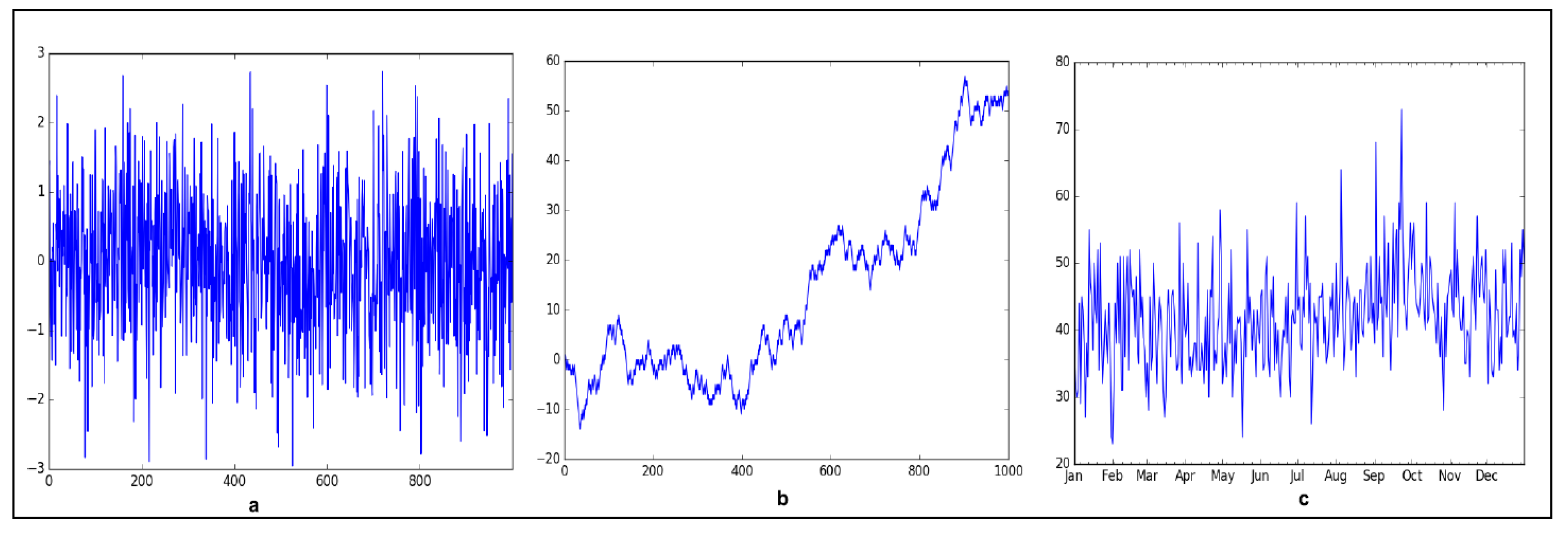
Figure 3.
Example of time series (TS). (a) Gaussian white noise (strictly stationary) (μ = 0, σ2 = k (constant), γ[τ] = 0 for all τ). (b) Random walk (non-stationary)—non-constant mean and variance. (c) Weakly stationary (μ ≠ 0, σ2 = k (constant), γ(t, s) = γ[τ] = X auto-covariance between any two points (t, s) is constant for fixed τ = t − s distance (lag)) as there is no obvious trend and repeating seasonality effects.
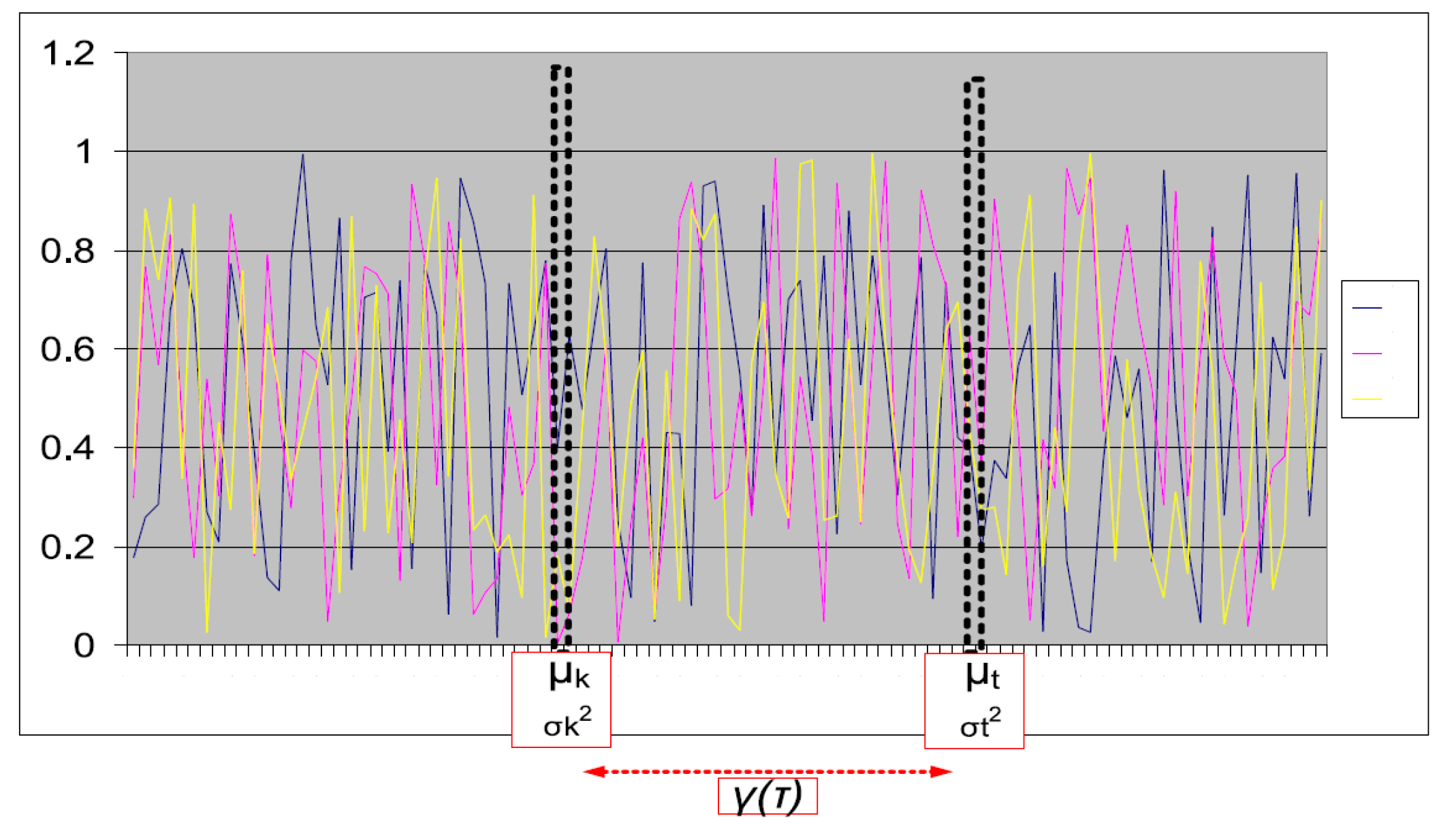
Figure 4.
Several time-series generated using the same stationary process or a random variable (X). Weakly stationary requires the non-zero mean (μ) and variance σ2 to be constant for all times (slices) e.g., t or k. In addition, the covariance (γ[τ]) must only be a function of temporal distance between any two points in time.
Figure 5.
Test HMI application in manual and auto-pilot mode. Process values are generated using AR(p), MA(q), and Gaussian noise process with trend and seasonal components. (a) Manual mode: process values displayed via array of lamp indicators. User tracks indication patterns by manually setting 8 toggle switches in same pattern until alarm indication (red lamp) goes off. (b) Auto-pilot mode: user tracking response to process values is modeled using a proportional-integral (PI) controller with random proportional gain. HMI process and user response was captured as a time-series data example of a diagram.
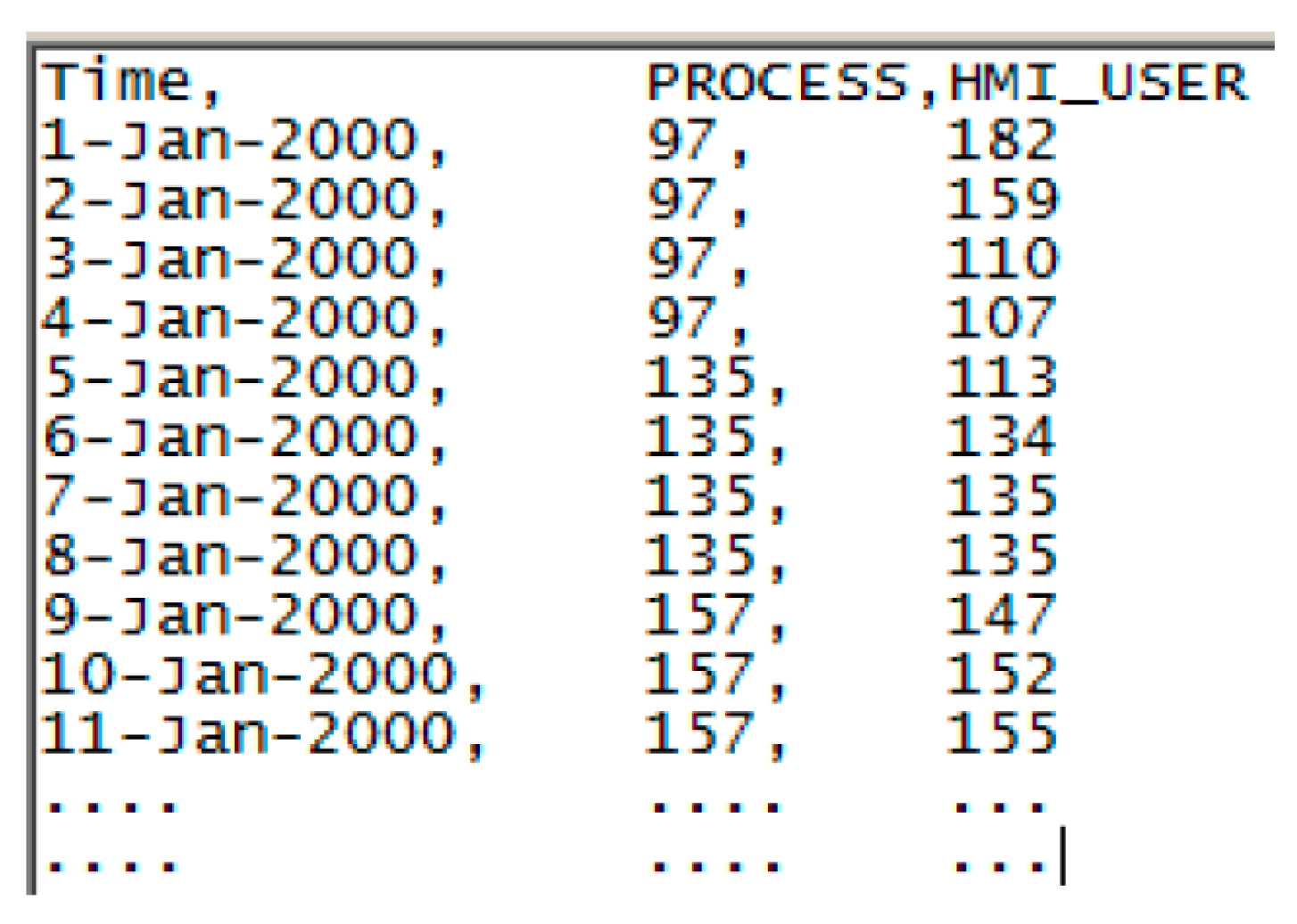
Figure 6.
Sample time-series data set. PROCESS and HMI_USER series dataset samples were limited to 8-bit integers.
Figure 6.
Sample time-series data set. PROCESS and HMI_USER series dataset samples were limited to 8-bit integers.
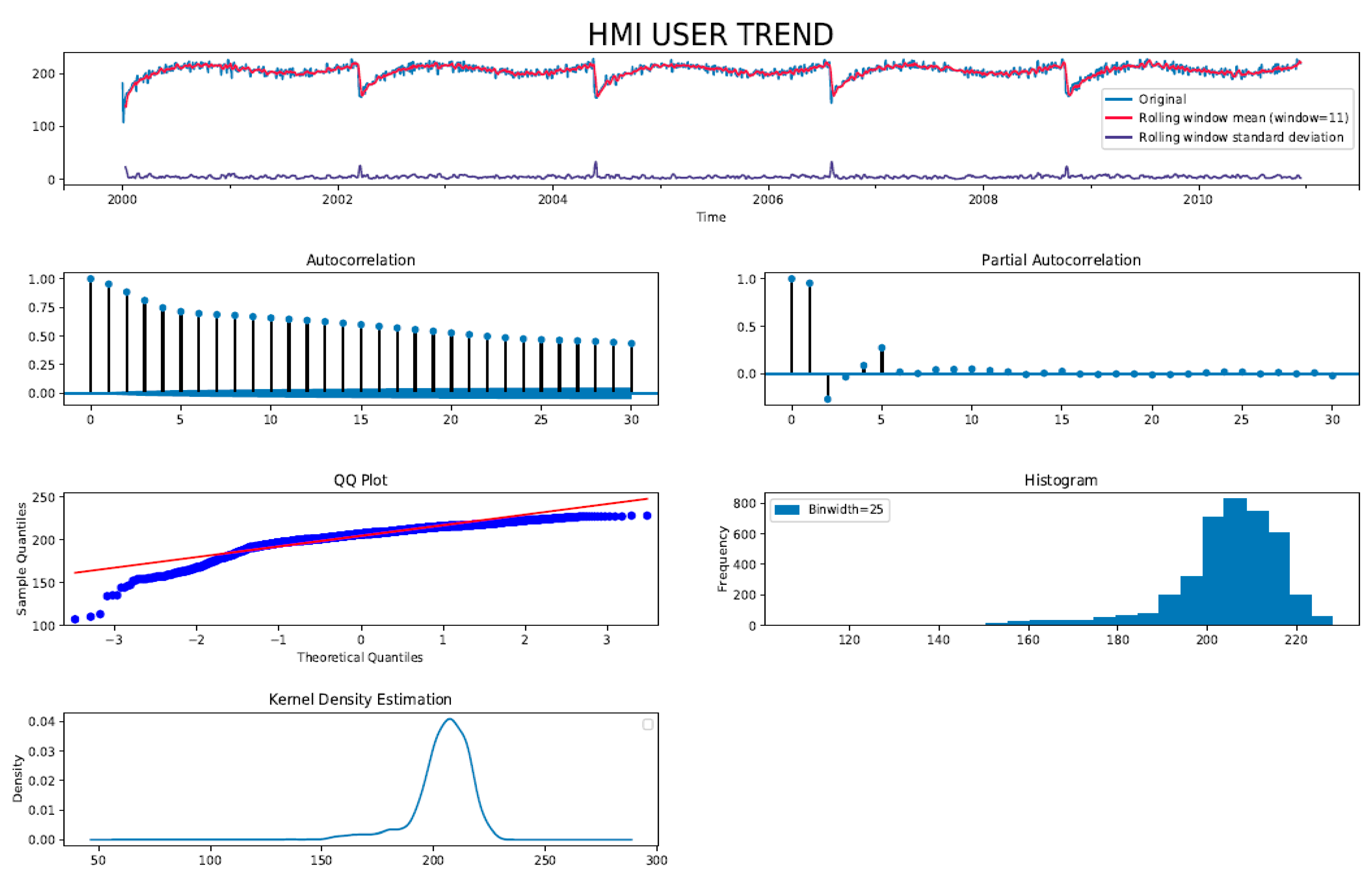
Figure 7.
Diagnostic plots of original the HMI_USER series dataset. Moving average mean shows seasonal trend therefore TS is non-stationary. TS is not random walk, since rolling standard deviation (variance) does not vary with time. Auto-Correlation Function (ACF) decays slowly indicative of seasonal trend. Partial Auto-Correlation Function (PACF) indicates a moving average (MA) process of finite lag. Quantile (QQ), histogram, and kernel density plots indicate a Gaussian-like distribution with a long tail suggesting presence of a periodic trend component in TS.
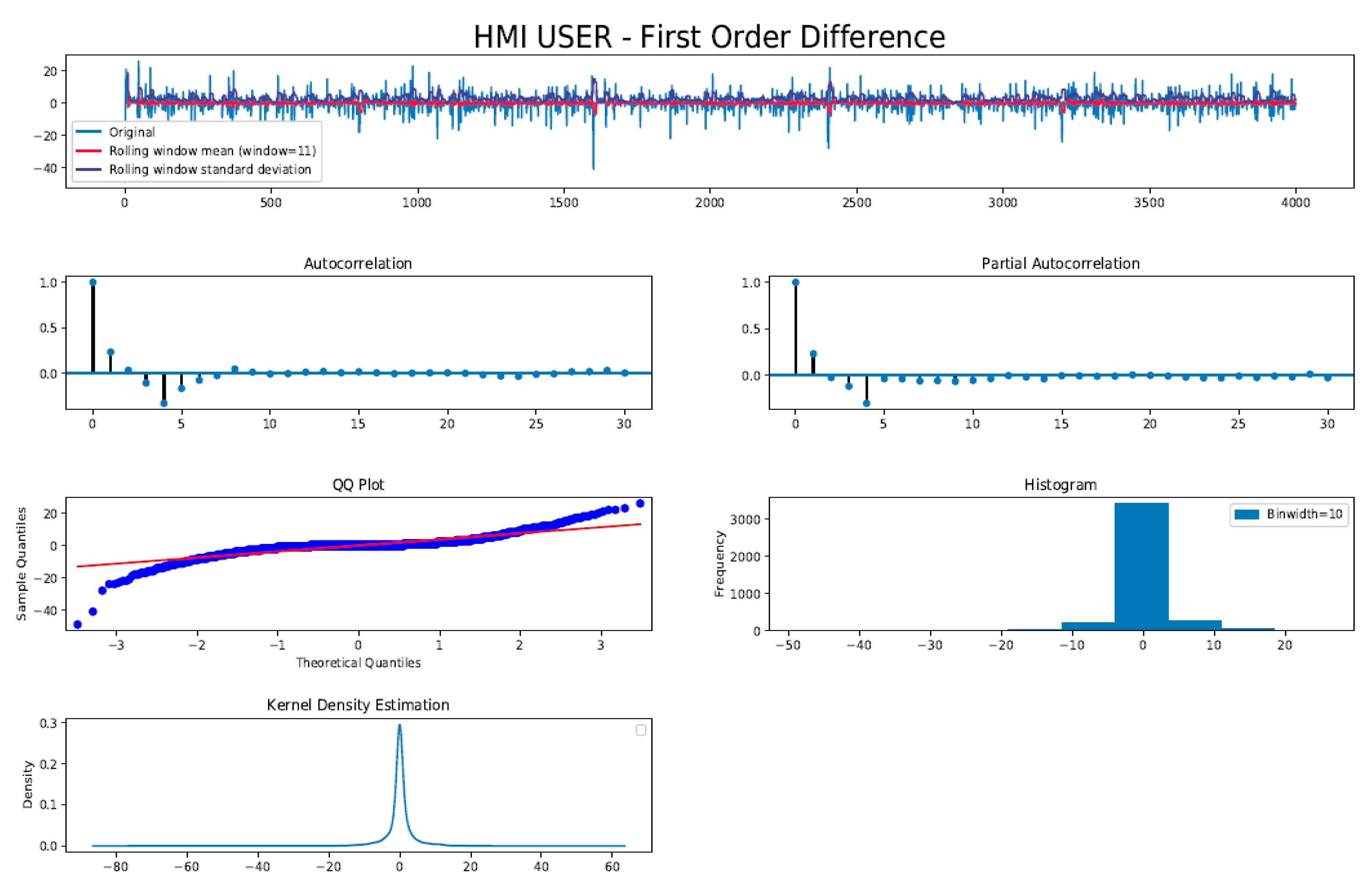
Figure 8.
Diagnostic plots of log first order difference of the HMI_User series dataset. Moving average mean no longer shows seasonal trend, therefore TS is closer to being stationary. Moreover, both rolling mean and standard deviation (variance) does not vary with time. ACF decays rapidly and cut off hard, indicative of AR(p) process. PACF also shows rapid decay after lag = 4 indicating MA(q) process. Quantile (QQ), histogram, and kernel density plots indicate a more Gaussian-like distribution with negligible tail suggesting the trend component has been minimized significantly.
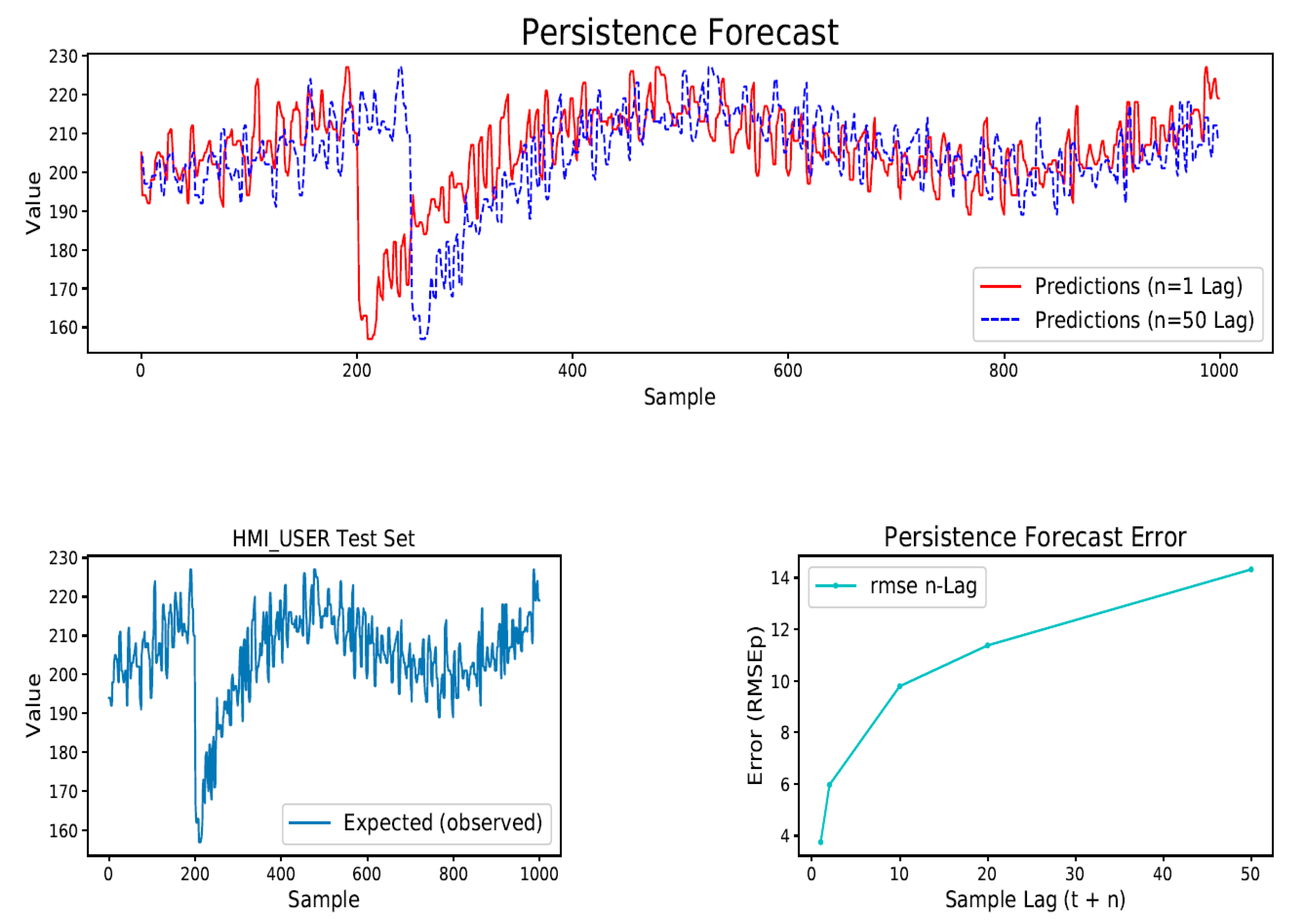
Figure 9.
Persistence (naive) forecast model plot for 50 lag. Root Mean Square Error (RMSE) of persistence model was used to ascertain the acceptable upper bound (worst case) of forecast error associated with the particular data set when using a forecast model.
Figure 9.
Persistence (naive) forecast model plot for 50 lag. Root Mean Square Error (RMSE) of persistence model was used to ascertain the acceptable upper bound (worst case) of forecast error associated with the particular data set when using a forecast model.
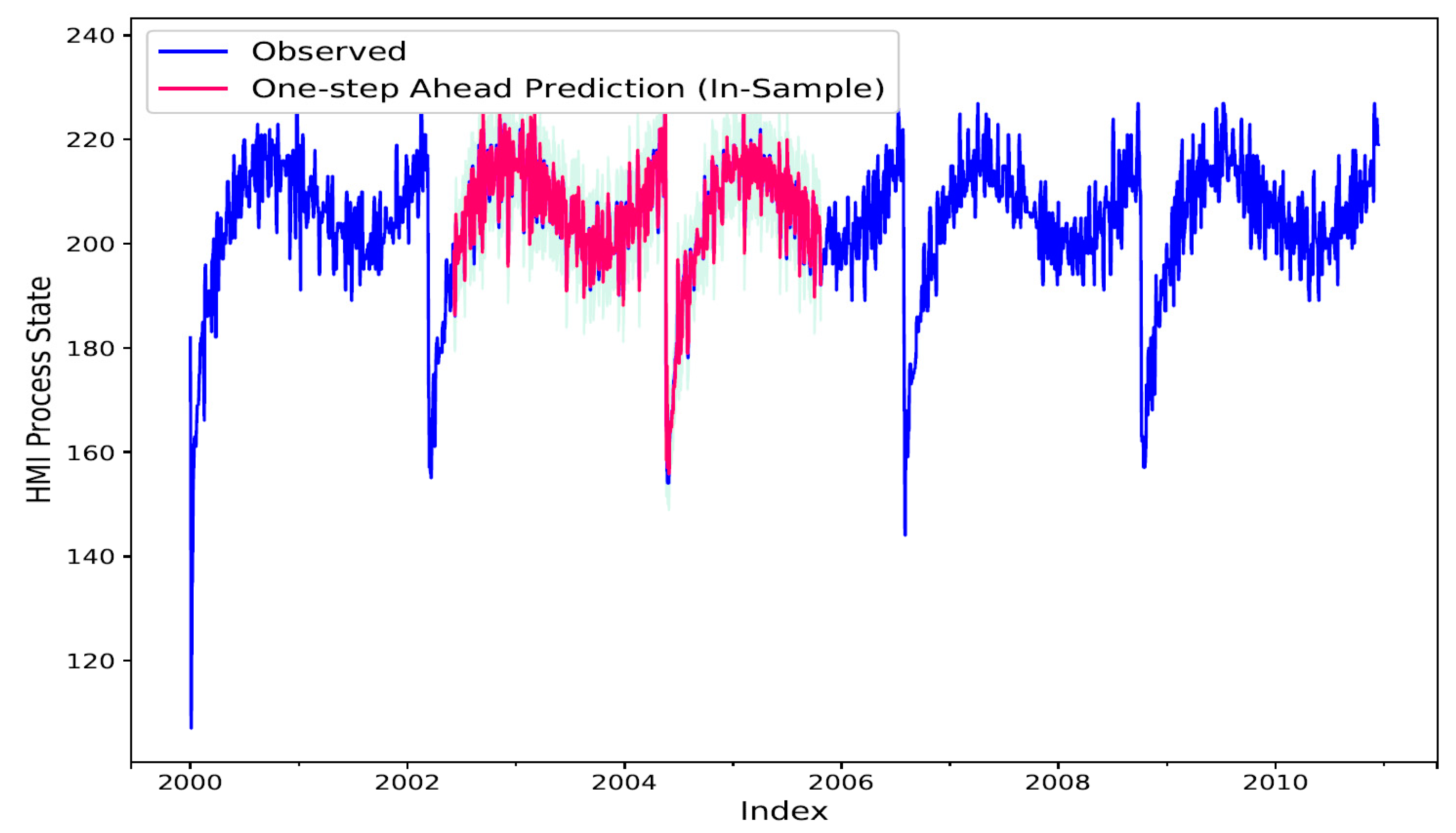
Figure 10.
In-sample (InS), Static 1-Step ahead forecast TS. TS (blue) shows observed actual values of the training set. TS (red) shows the InS forecasted values which closely track the training set. Light blue background shows confidence interval bounds for the forecast TS.
Figure 10.
In-sample (InS), Static 1-Step ahead forecast TS. TS (blue) shows observed actual values of the training set. TS (red) shows the InS forecasted values which closely track the training set. Light blue background shows confidence interval bounds for the forecast TS.
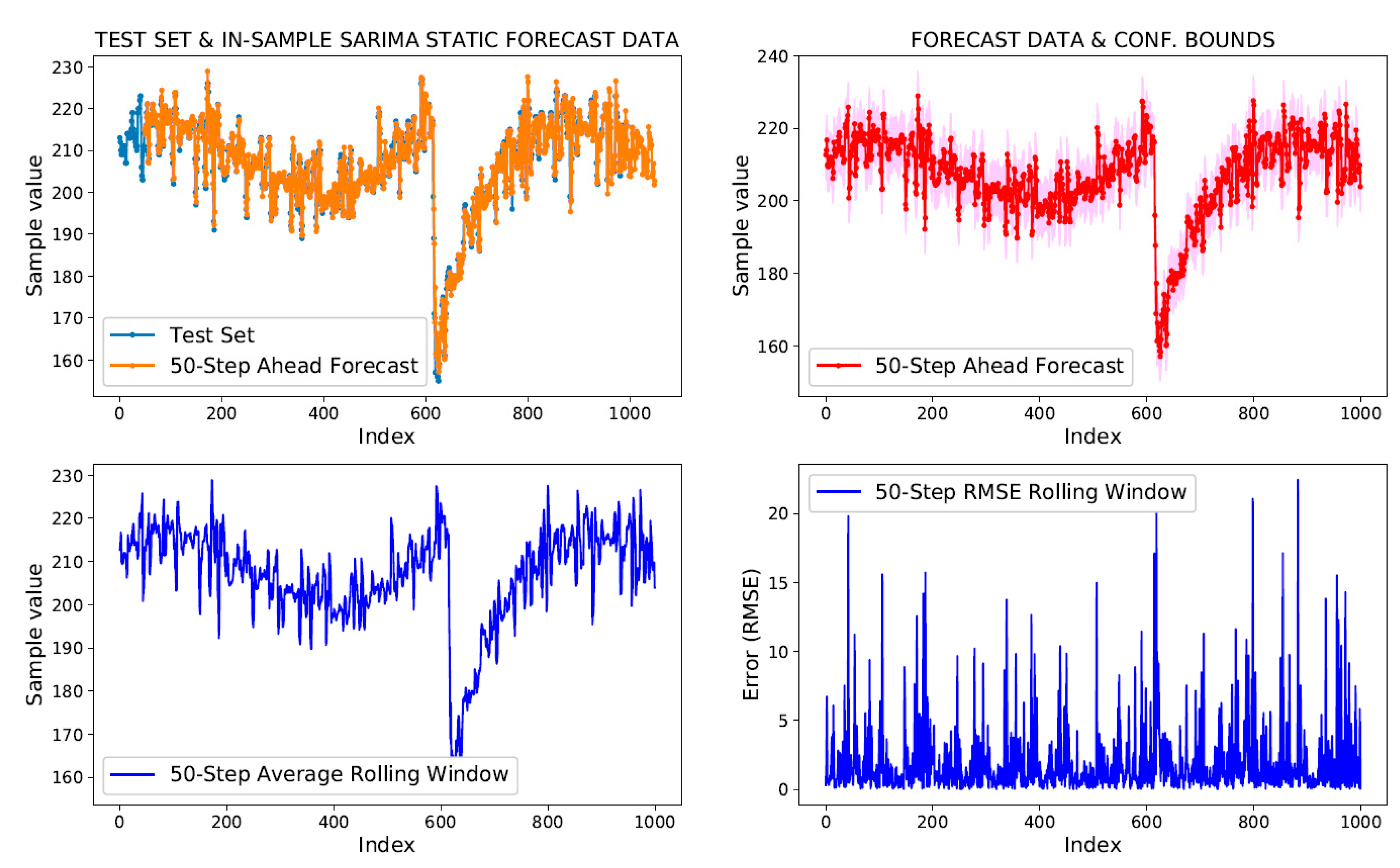
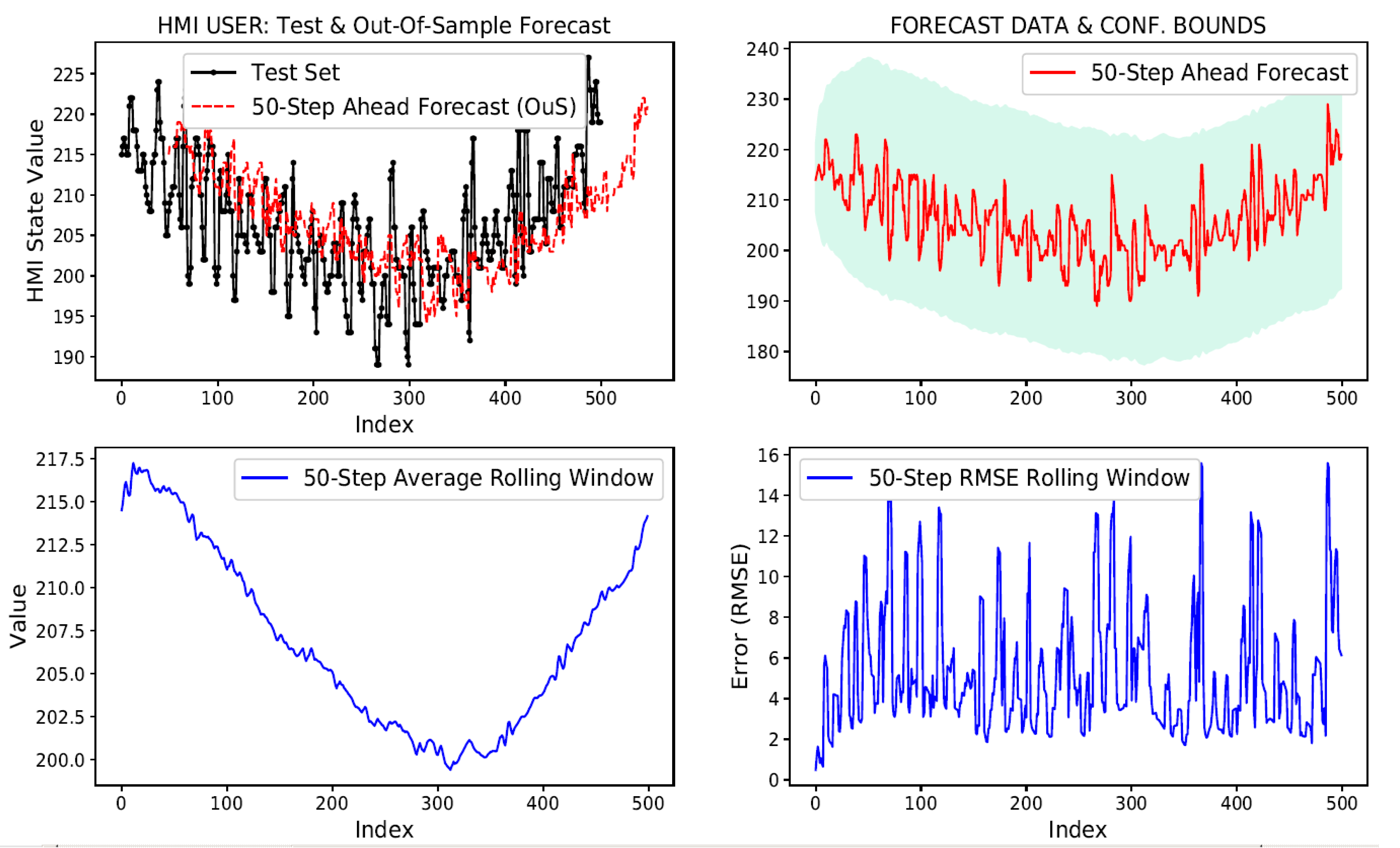
Figure 11.
In-sample (InS) static 50-Step ahead forecast. Top-left plot shows 50-step ahead predicted samples overlaid on the actual InS test set. Top-right plot shows the forecast TS with per sample confidence interval as background colour. Bottom (right and left) plots show rolling window metrics: average and RMSE, respectively, for the 50-Step ahead forecast.
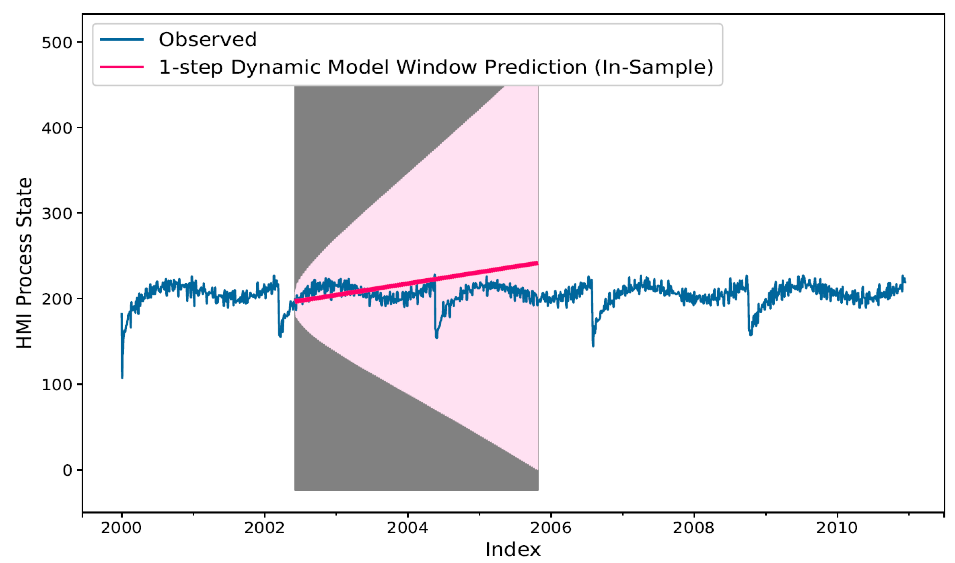
Figure 12.
InS 1-Step ahead static model in dynamic mode forecast (red bold line). The confidence interval (prediction error) associated with forecast values may be seen in background as a lighter shade of pink area on the plot, which deviates with a constant up trend indicative of accumulation of forecast error per previously predicted values.
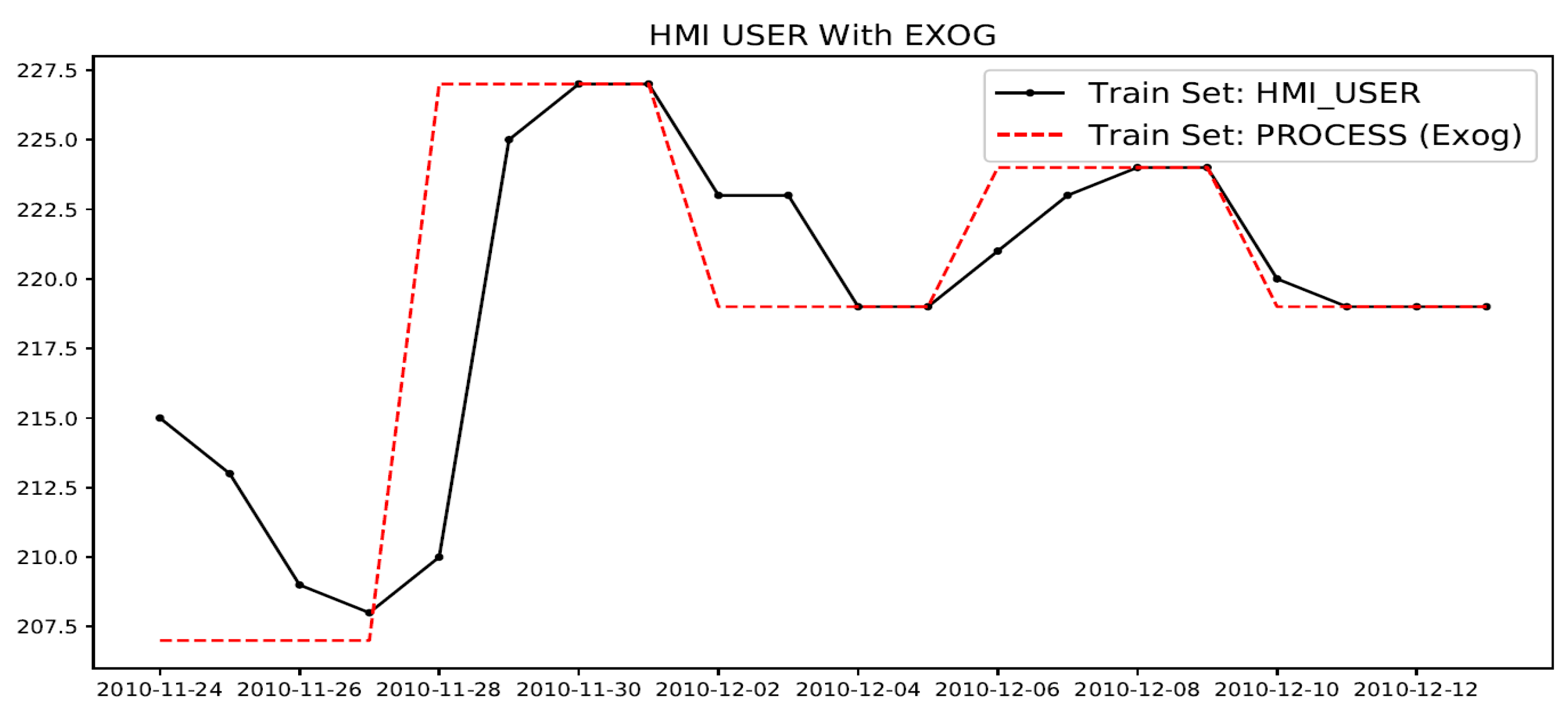
Figure 13.
Example showing HMI_USER (variable to be modeled) and its exogenous (Exog.) predictor variable: PROCESS state.
Figure 13.
Example showing HMI_USER (variable to be modeled) and its exogenous (Exog.) predictor variable: PROCESS state.
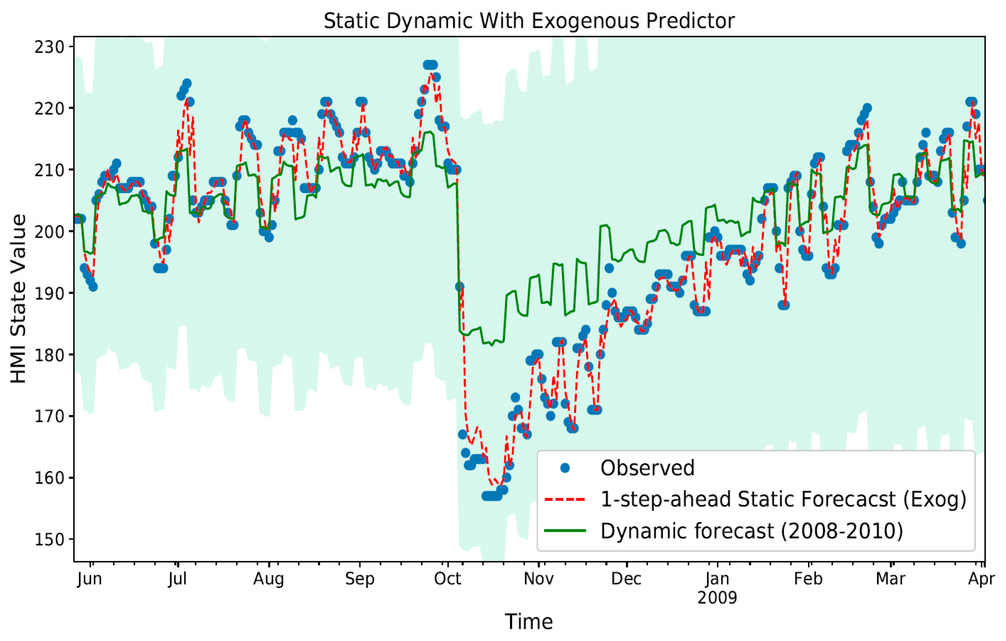
Figure 14.
In sample 1-Step ahead static with normal and dynamic mode forecast with exogenous predictor (PROCESS) variable. The confidence interval associated with the static dynamic model trend (bold green line) may be seen in background as a light blue shade on the plot area.
Figure 14.
In sample 1-Step ahead static with normal and dynamic mode forecast with exogenous predictor (PROCESS) variable. The confidence interval associated with the static dynamic model trend (bold green line) may be seen in background as a light blue shade on the plot area.
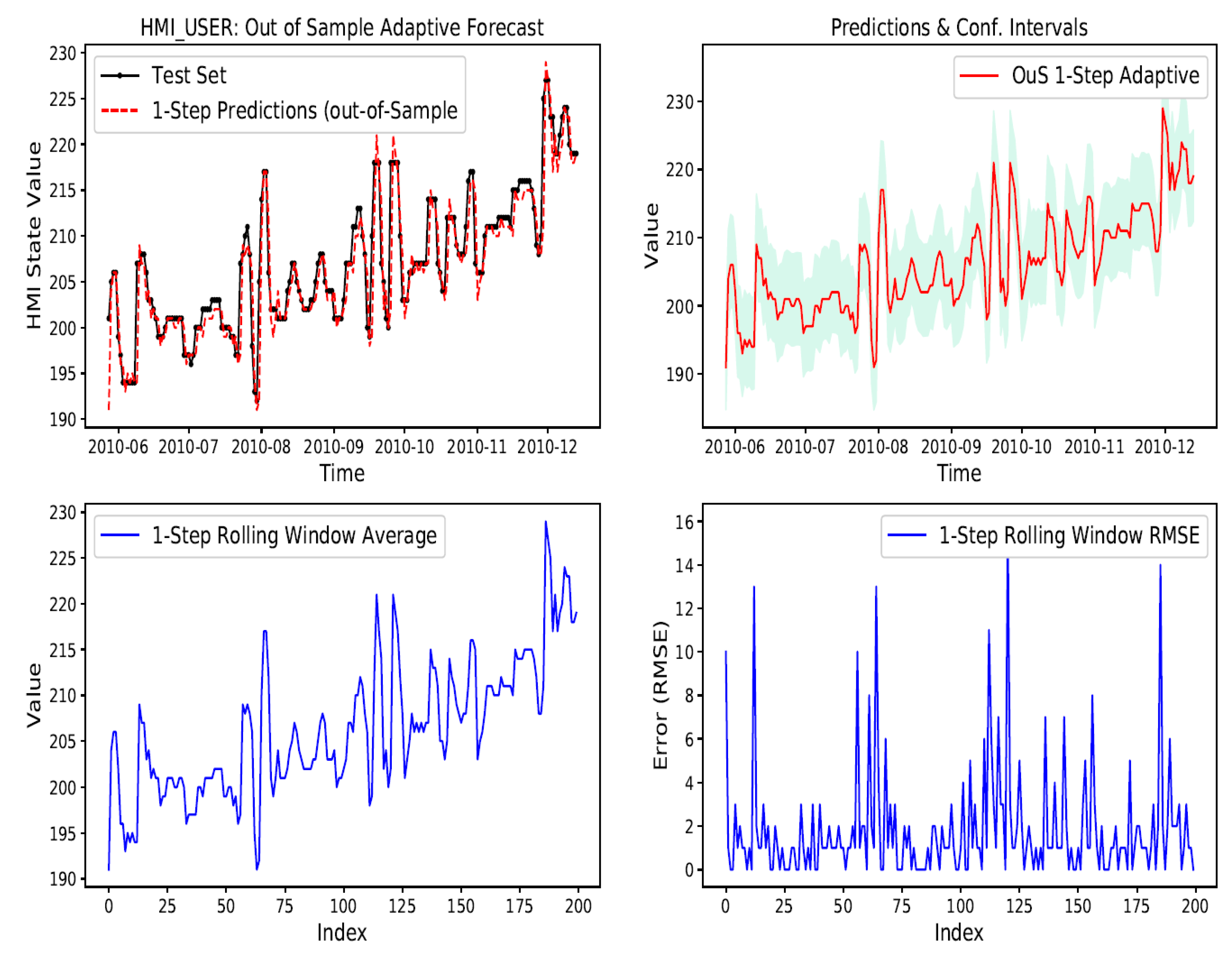
Figure 15.
Out-of-Sample adaptive 1-Step ahead prediction for 200 sample run lengths shows close tracking.
Figure 15.
Out-of-Sample adaptive 1-Step ahead prediction for 200 sample run lengths shows close tracking.
Figure 16.
Out-of-sample adaptive 50-Step ahead prediction for 500 sample run lengths scale attenuated.
Figure 16.
Out-of-sample adaptive 50-Step ahead prediction for 500 sample run lengths scale attenuated.
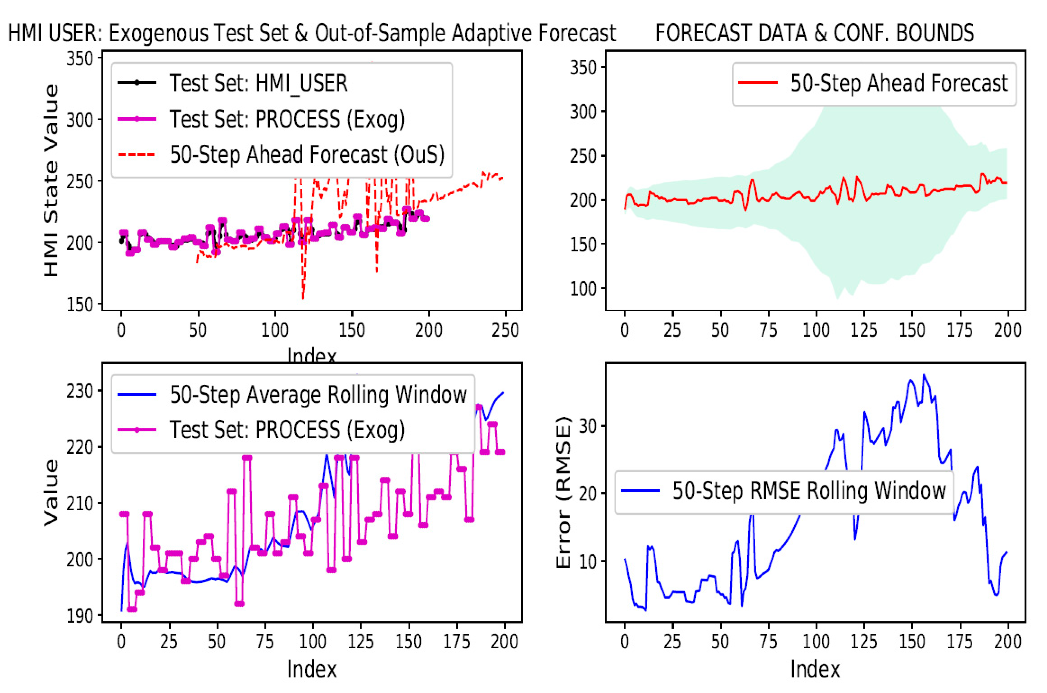
Figure 17.
Out-of-sample adaptive 50-Step ahead for 500 sample runs with exogenous input.
Figure 17.
Out-of-sample adaptive 50-Step ahead for 500 sample runs with exogenous input.
Table 1.
Persistence n-Lag RMSEp.
Table 1.
Persistence n-Lag RMSEp.
| n-Lag | RMSEp |
|---|
| 1 | 3.75 |
| 2 | 5.96 |
| 10 | 9.78 |
| 20 | 11.37 |
Table 2.
In-sample static n-Step RMSE.
Table 2.
In-sample static n-Step RMSE.
| n-Step | RMSE |
|---|
| 1 | 3.41 |
| 2 | 3.39 |
| 10 | 3.42 |
| 20 | 3.40 |
Table 3.
Out-of-sample adaptive 1-Step RMSE.
Table 3.
Out-of-sample adaptive 1-Step RMSE.
| Sample Run | RMSE |
|---|
| 10 | 1.82 |
| 20 | 3.79 |
| 50 | 2.93 |
| 200 | 3.18 |
Table 4.
OuS adaptive n-Step RMSE.
Table 4.
OuS adaptive n-Step RMSE.
| n-Step | Sample Run | RMSE |
|---|
| 1 | 20 | 3.79 |
| 2 | 20 | 4.24 |
| 2 | 200 | 3.63 |
| 4 | 20 | 4.81 |
| 4 | 500 | 5.19 |
| 10 | 10 | 2.20 |
| 10 | 200 | 4.47 |
| 10 | 500 | 4.97 |
| 20 | 500 | 5.20 |
| 50 | 500 | 5.20 |
Table 5.
OuS adaptive dynamic n-Step RMSE.
Table 5.
OuS adaptive dynamic n-Step RMSE.
| n-Step | Sample Run | RMSE |
|---|
| 4 | 10 | 3.01 |
| 10 | 200 | 5.09 |
| 1 | 500 | 5.02 |
| 4 | 500 | 5.45 |
| 20 | 500 | 5.42 |
| 50 | 500 | 5.67 |
Table 6.
OuS adaptive Exog. n-Step RMSE.
Table 6.
OuS adaptive Exog. n-Step RMSE.
| n-Step | Sample Run | RMSE |
|---|
| 1 | 200 | 3.12 |
| 2 | 200 | 3.70 |
| 4 | 200 | 4.56 |
| 10 | 200 | 4.78 |
| 20 | 200 | 5.40 |
| 50 | 200 | 9.42 |
Table 7.
OuS adaptive dynamic Exog. n-Step RMSE.
Table 7.
OuS adaptive dynamic Exog. n-Step RMSE.
| n-Step | Sample Run | RMSE |
|---|
| 1 | 200 | 5.40 |
| 2 | 200 | 5.96 |
| 4 | 200 | 6.48 |
| 10 | 200 | 5.92 |
| 20 | 200 | 6.34 |
| 50 | 200 | 9.62 |
Table 8.
Static ARIMA model limitations.
Table 8.
Static ARIMA model limitations.
| Limitation | Performance | Rationale |
|---|
Out-of-Sample (OuS)
n-Step Ahead Performance | Poor | ARIMA model parameters cannot be sufficiently optimized for doing longer run OuS predictions. |
| Dynamic Mode for InS and OuS Performance | Poor | Yields higher error than same p-lag persistence RMSEp value.
This is owing to model not being re-fitted which causes forecast errors to accumulate and amplify. |
Table 9.
Adaptive ARIMA model limitations.
Table 9.
Adaptive ARIMA model limitations.
| Limitation | Performance | Rationale |
|---|
| Multi-variate (Exogenous) time-series prediction support | Poor | Adaptive model with dynamic mode yields consistent RMSE values for n-step ahead predictions; however, it yields higher RMSE values for longer n-step ahead prediction. |


