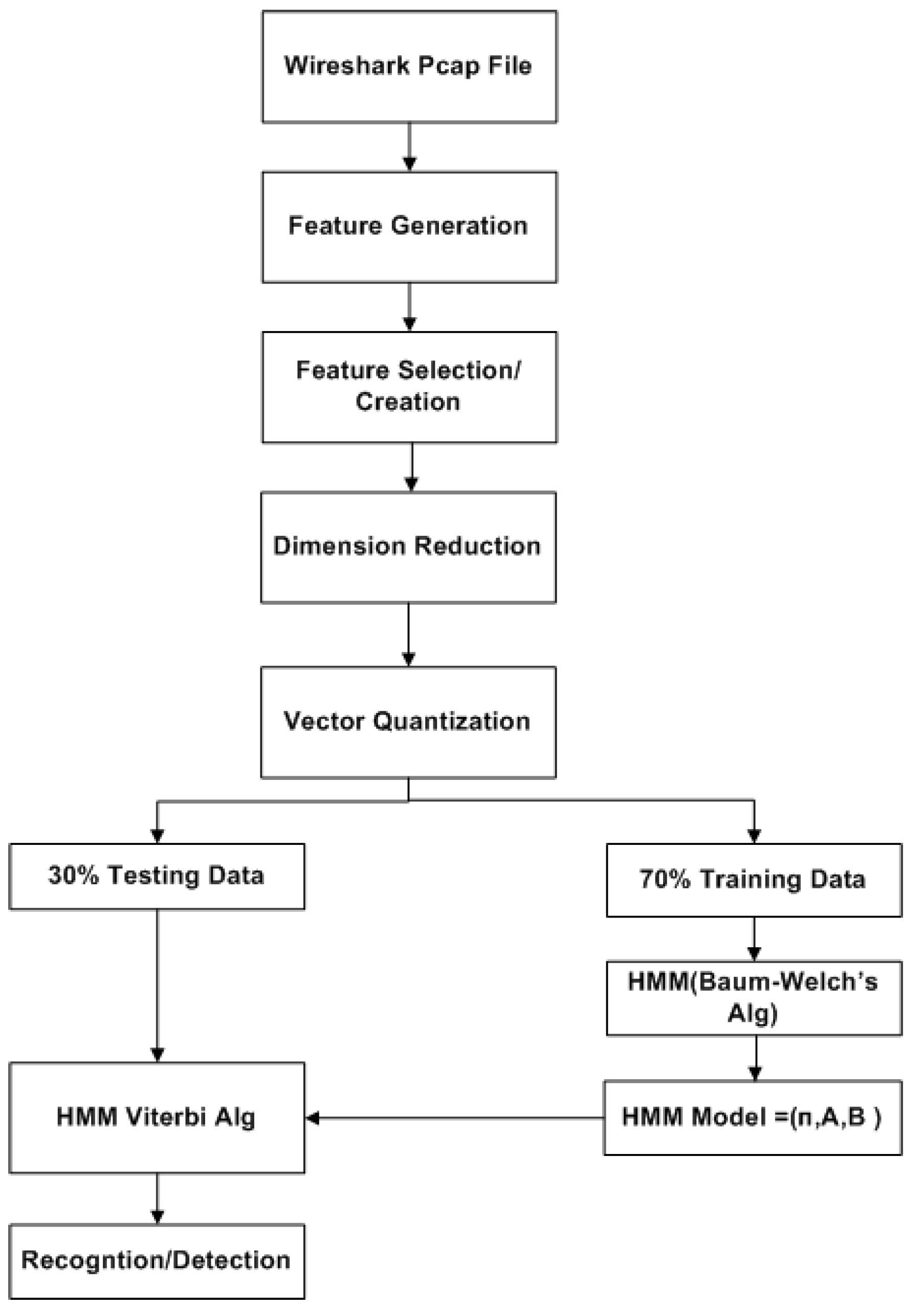
A challenge in applying the Markov model to intrusion detection systems is the lack of a standard method for the translation of the observed network packet data into meaningful Markov model. The first step towards building an IDS based on multiple layers of Hidden Markov Models involves processing network traffic into meaningful observations.
2.1. CICIDS2017 Data Processing
Datasets such as DARPA98-99(Lincoln Laboratory 1998–1999), KDD’99 (University of California, Irvine 1998–1999), DEFCON (The Shmoo Group, 2000–2002) UMASS (University of Massachusetts 2011), ISC2012 (University of New Brunswick 2012) and ADFA’13 (University of New South Wales 2013), to name a few, have been used by several researchers to validate their IDS’s designs and approaches. Those datasets have shortcomings associated with them. For example, DARPA98-99 and KDD’99 are outdated and unreliable as several flows are redundant; NSL-KDD has been used to replace KDD’99 by removing the significant redundancy. The work in Reference [
10] further analyzed the KDD’99 and presented new proofs to these existing inconsistencies. CAIDA (Center of Applied Internet Data Analysis 2002–2016) traffic payloads are heavily anonymized. ADFA’13 lacks attack diversity and variety. Besides to these popular datasets among various researchers, several others are also explored in Reference [
11].
Most of the datasets are also simulate attacks which are multi-stage. The CICIDS2017 dataset is designed to cover what are commonly referred as the eleven criteria for IDS dataset evaluation framework (Network, traffic, Label, Interaction, capture, Protocols, Attack diversity, anonymization, heterogeneity, features and metadata). The details of this dataset compared to the commonly available IDS evaluation datasets is presented in Reference [
12].
For testing the modeled IDS in this work, a dataset is prepared from the CICIDS2017 dataset. This dataset covers eleven criteria which are necessary in building a reliable benchmark dataset. It contains very common attacks such as XSS, Port scan, Infiltration, Brute Force, SQL Injection, Botnet DoS and DDoS. The dataset is made up of 81 features including the label and it is publicly available in Canadian Institute for Cybersecurity website [
13]. Some of these features are directly extracted while others are calculated for both normal (benign) and anomalous flows using the CICFlowMeter [
14].
The CICIDS2017 dataset comprises 3.1 million flow records and it covers five days. It includes the following labeled attack types: Benign, DoS Hulk, Port Scan, DDoS, DoS, FTP Patator, SSH Patator, DoS Slow Loris, DoS Slow HTTP Test, Botnet, Web Attack: Brute Force, Web Attack: Infiltration, Web Attack: SQL Injection and Heartbleed. The portion of the “Thursday-WorkingHours-Morning-webattack” is used to create the training and testing dataset which constitutes “BENIGN”, “SSH Patator” and “Web Attack-Brute Force” traffic.
2.3. Feature Extraction/Dimension Reduction
On the other hand, dimension reduction is one form of transformation whereby a new set of features is extracted. This feature extraction process extracts a set of new features from the initial features through some functional mapping [
17].
Feature extraction, also known as dimension reduction, is applied after feature selection and feature creation procedures on the original set of features. Its goal is to extract a set of new features through some functional mapping. If we initially have n features (or attributes), , after feature selection and creation, feature extraction results in a new set of features, where and is a mapping function.
PCA is a classic technique which is used to compute a linear transformation by mapping data from a high dimensional space to a lower dimension. The original n features are replaced by another set of m features that are computed from a linear combination of these initial features.
Principal Component Analysis is used to compute a linear transformation by mapping data from a high dimensional space to a lower dimension. The first principal component contributes the highest variance in the original dataset and so on. Therefore, in the dimension reduction process, the last few components can be discarded as it only results in minimal loss of the information value [
18].
The main goals of PCA:
Extract the maximum variation in the data.
Reduce the size of the data by keeping only the significant information.
Make the representation of the data simple.
Analyze the structure of the variables (features) and observations.
Generally speaking, PCA provides a framework for minimizing data dimensionality by identifying principal components, linear combinations of variables, which represent the maximum variation in the data. Principal axes linearly fit the original data so the first principal axis minimizes the sum of squares for all observational values and maximally reduces residual variation. Each subsequent principal axis maximally accounts for variation in residual data and acts as the line of best fit directionally orthogonal to previously defined axes. Principal components represent the correlation between variables and the corresponding principal axes. Conceptually, PCA is a greedy algorithm fitting each axis to the data while conditioning upon all previous axes definitions. Principal components project the original data onto these axes, where these axes are ordered such that Principal Component 1 () accounts for the most variation, followed by for variables (dimensions).
Steps to compute PCA using Eigen Value Decomposition (EVD):
From each of the dimensions subtract the mean.
Determine the covariance matrix.
Determine the eigenvalues and eigenvectors of the calculated covariance matrix.
Reduce dimensionality and construct a feature vector.
Determine the new data.
The PCA procedure used applies Singular Value Decomposition (SVD) instead of Eigenvalue Decomposition (EVD) [
19]. SVD is numerically more stable as it avoids the computation of the covariance matrix which is an expensive operation.
Singular Value Decomposition (SVD) for Principal Component Analysis (PCA)
Any matrix X of dimension N × d can be uniquely written as
Where
r is the rank of matrix X (i.e., the number of linearly independent vectors in the matrix)
U is a column- orthonormal matrix of dimension
∑ is a diagonal matrix of dimension where σi’s (the singular values) are sorted in descending order across the diagonal.
V is a column- orthonormal matrix of dimension .
Given a data matrix X, the PCA computation using SVD is as follows
For a rank , square, symmetric matrix
- ▪
is the set of orthonormal Eigenvectors with Eigenvalues
The principal components of are the eigenvectors of
are positive real and termed singular values
is the set of orthonormal vectors defined by
- ▪
- ▪
(the “value” form of SVD) where
∑ is and diagonal
- ▪
σi are called singular values of . It is assumed that σ1 ≥ σ2 ≥ … ≥ ≥ 0 (rank ordered).
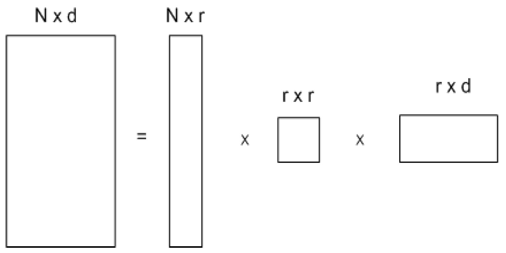
For N > (r = d), the bottom N-r rows of ∑ are all zeros which will be removed and the first r rows of ∑ and the first r columns of U will be kept which results in the decomposition shown in
Figure 2.
PCA and SVD relation
Let be the SVD of matrix X and be its covariance matrix of dimension d x d. The Eigenvalues of C are the same as the right singular vectors of X.
This can be shown with the following proof:
As C is symmetric, hence C = VΛVT. As a result, the eigenvectors of the covariance matrix are the same as the matrix V (right singular vectors) and the eigenvalues of C can be determined from the singular values
PCA using EVD and SVD can be summarized as follows:
Objective: project the original data matrix X using the largest m principal components, .
PCA:
SVD:
3. Project the data in an m dimensional space: Y = XV
To perform dimension reduction and form a feature vector using PCA, order the eigenvalues from the highest to lowest by value. This ordering places the components in order of significance to the variance of the original data matrix. Then we can discard components of less significance. If a number of eigenvalues are small, we can keep most of the information we need and loss a little or noise. We can reduce the dimension of the original data.
E.g. we have data of
d dimensions and we choose only the first
r eigenvectors.
Since each PC is orthogonal, each component independently accounts for data variability and the Percent of Total Variation Explained (PTV) is cumulative. PCA offers as many principal components as variables in order to explain all variability in the data. However, only a subset of these principal components is notably informative. Since variability is shifted into leading PCs, many of the remaining PCs account for little variation and can be disregarded to retain maximal variability with reduced dimensionality.
For example, if 99% total variation should be retained in the model for
d dimensional data, the first
r principal components should be kept such that
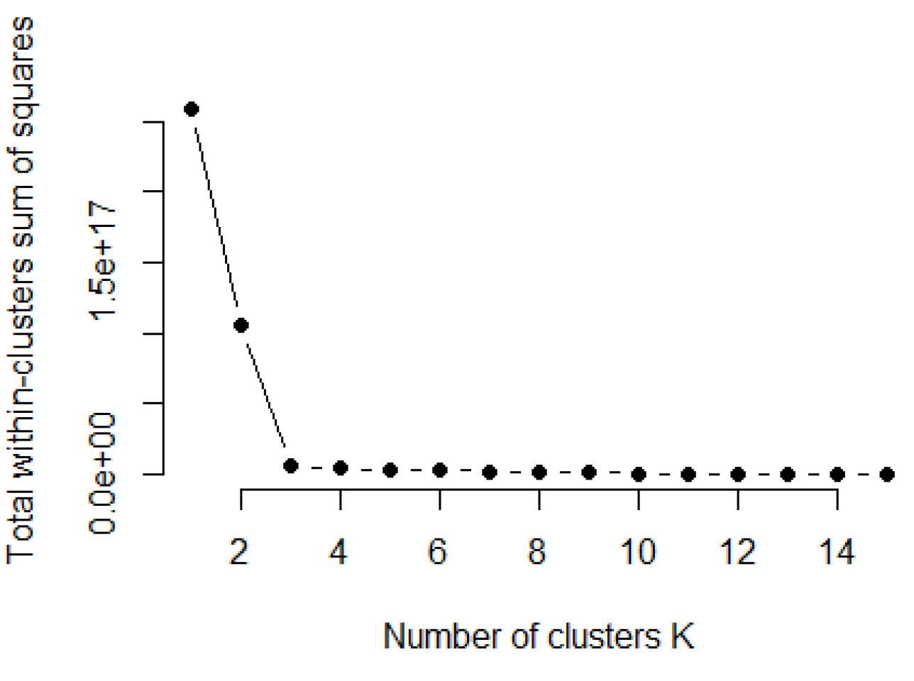
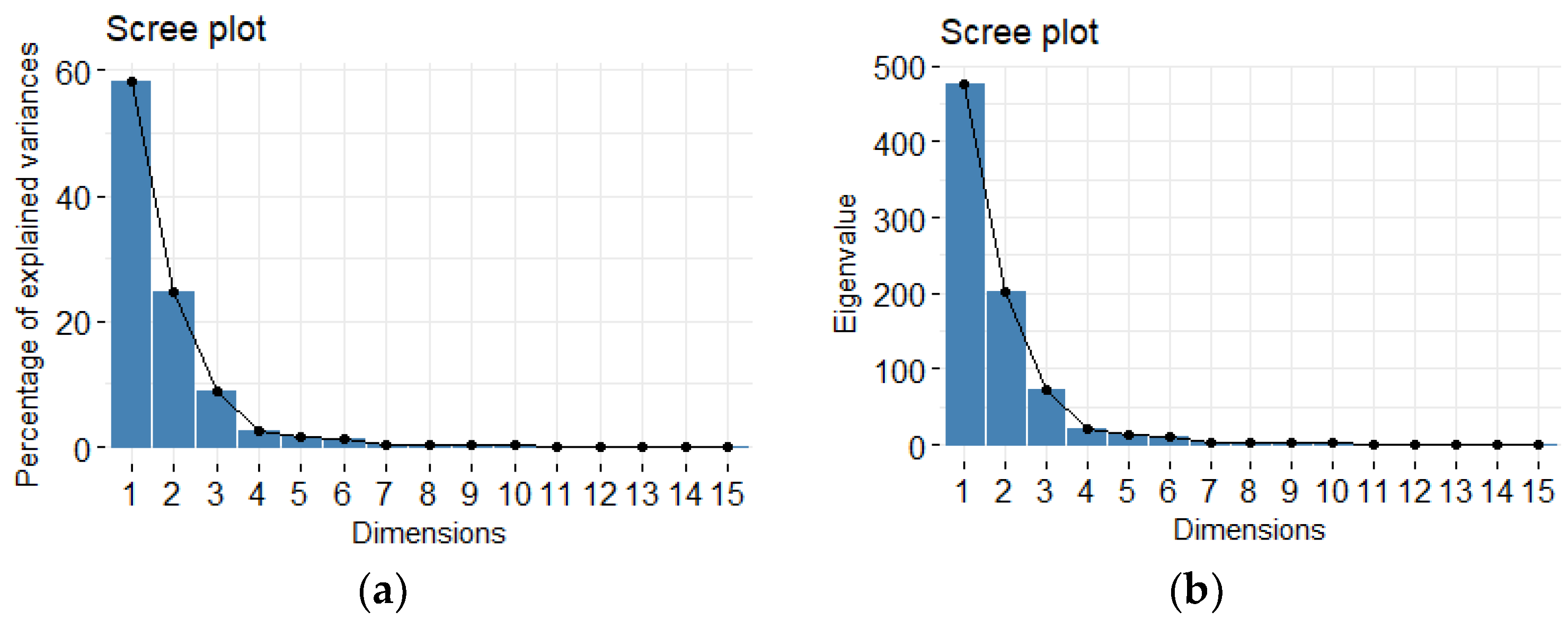
PTV acts as the signal to noise ratio, which flattens with additional components. Typically, the number of informative components r is chosen using one of three methods: (1) Kaiser’s eigenvalue > 1; (2) Cattell’s scree plot; or (3) Bartlett test of sphericity.
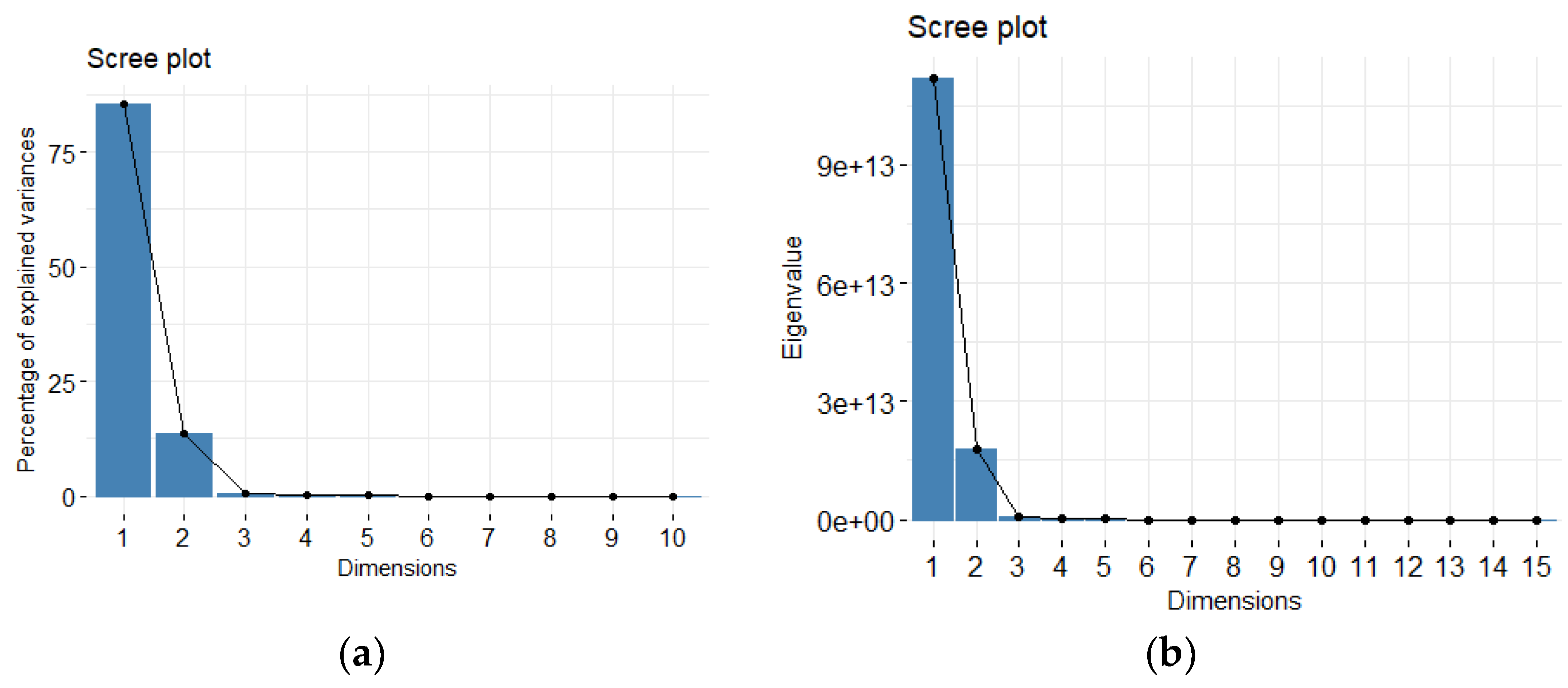
The amount of variation in redundant data decreases from the first principal component onwards. There are several methods to compute the cut off value for retaining the sufficient number of principal components out of all
p components. In this work, we use the Cattell’s scree plot, which plots the eigenvalues in decreasing order [
20]. The number of principal components to be kept is determined by the elbow where the curve becomes asymptotic and additional components provide little information. Another method is the Kaiser criterion Kaiser [
21] which retains only factors with eigenvalues >1.


